
Estimating the Competitive Storage Model with Stochastic Trends in Commodity Prices


1
Department of Mathematics and Physics, University of Stavanger, 4036 Stavanger, Norway
2
Institute of Econometrics and Statistics, University of Cologne, Albertus-Magnus-Platz, 50937 Cologne, Germany
3
Department of Safety, Economics and Planning, University of Stavanger, 4036 Stavanger, Norway
*
Author to whom correspondence should be addressed.
Econometrics 2021, 9(4), 40; https://0-doi-org.brum.beds.ac.uk/10.3390/econometrics9040040
Submission received: 28 April 2021
/
Revised: 30 October 2021
/
Accepted: 2 November 2021
/
Published: 5 November 2021
Abstract
:We propose a State-Space Model (SSM) for commodity prices that combines the competitive storage model with a stochastic trend. This approach fits into the economic rationality of storage decisions and adds to previous deterministic trend specifications of the storage model. For a Bayesian posterior analysis of the SSM, which is nonlinear in the latent states, we used a Markov chain Monte Carlo algorithm based on the particle marginal Metropolis–Hastings approach. An empirical application to four commodity markets showed that the stochastic trend SSM is favored over deterministic trend specifications. The stochastic trend SSM identifies structural parameters that differ from those for deterministic trend specifications. In particular, the estimated price elasticities of demand are typically larger under the stochastic trend SSM.
1. Introduction
How to deal with trends when confronting economic theories with real-world data is an important issue. This is a well-known problem in empirical macroeconomics, where structural parameters of business cycle models are often estimated on data that have been filtered in order to remove variation at frequencies that the model is not intended to explain, such as low-frequency trend variations and seasonal fluctuations (DeJong and Dave 2011; Sala 2015). For an overview of alternatives to the use of prefiltered data in order to address this general problem, see Canova (2014).
In the competitive storage model for commodity prices introduced by Gustafson (1958), the situation is similar to that of business cycle models. The rational expectations equilibrium implied by the solution of this model is only known to exist in a stationary market. Accordingly, it is a model for describing dynamic price adjustments towards an exogenously given fixed steady-state equilibrium. However, it cannot explain low-frequency price movements due to persistent shocks. This is problematic when attempting to estimate the structural parameters of the model using commodity price data, since time series of commodity prices typically display a strongly persistent behavior in the price level, so that nonstationarity cannot be rejected when using conventional statistical tests (Gouel and Legrand 2017; Wang and Tomek 2007). As a result, the estimates for the structural parameters, which determine quantities such as the price elasticity of demand and storage costs, are likely to be biased. This issue was recognized by Deaton and Laroque (1995) in one of the earliest attempts to directly estimate the structural parameters of the storage model.
This paper proposes an approach to estimate the structural parameters of the competitive commodity storage model using a State-Space Model (SSM) for commodity prices, which decomposes the observed price into a stationary component, which is due to the storage model, and a stochastic trend component included to capture low-frequency price variations the storage model is unable to explain. Using a stochastic trend specification to account for nonstationary price data, our empirical approach aims at fitting into the economic rationality of the stationary storage model so that it preserves theoretical coherence, promising meaningful estimates of the structural parameters. Such a fit results from the fact that a stochastic trend that scales equilibrium prices can be isolated in the storage model by assuming that the innovations to the trend do not interfere with the agents’ equilibrium storage decisions. In the baseline storage model, unrestricted equilibrium storage decisions lead to an intertemporal pricing restriction of the form , where is the rational period-t expectation of the commodity price and represents some discount factor. Thus, a stochastic price scaling will not impair the equilibrium storage decisions if . This generically identifies stochastic trends as shifts in the price levels that do not interfere with intertemporal stock allocations and enables a coherent integration of the stationary rational expectations equilibrium into a nonstationary environment. Thus, it provides the theoretical basis of our empirical SSM approach, which jointly identifies the trend parameters and the structural parameters of the storage model.
The measurement equation, as well as the state transition equation of our SSM model are nonlinear and discontinuous in the latent states so that the likelihood is analytically intractable. To overcome this difficulty, we used a Markov Chain Monte Carlo (MCMC) algorithm for a Bayesian posterior analysis based on the Particle Marginal Metropolis–Hastings (PMMH) approach (Andrieu et al. 2010), which employs a particle filter inside a standard Metropolis–Hastings procedure to obtain a Monte Carlo (MC) estimate of the likelihood. This particle filter can also be applied to compute MC estimates for the predicted latent states, which we exploited for diagnostic checks of the SSM model.
With our proposed approach, we contribute to the literature concerned with the general problem of adapting stationary economic models to nonstationary data, and more specifically to the problem of estimating the structural parameters of the competitive storage model on nonstationary commodity price data. Legrand (2019) identified reliable estimation as one of the main issues of structural models for commodity prices. Early attempts at estimating the structural parameters revealed that fitted competitive storage models are not able to satisfactorily approximate the observed strong serial dependence in commodity price data, indicating misspecification of the empirical model and casting doubt on the reliability of the parameter estimates (Deaton and Laroque 1995). Suggested solutions to this problem include ad hoc enrichments of the dynamic structure of the storage model by including weakly dependent supply shocks (Deaton and Laroque 1996; Kleppe and Oglend 2017) or the tuning of the grid for the commodity stock state variable, used for approximating the policy function (Cafiero et al. 2011). Other approaches replace the estimation techniques applied in early empirical implementations of the storage model, such as the pseudo Maximum Likelihood (ML) procedure of Deaton and Laroque (1996), by more sophisticated ones, such as the ML technique developed by Cafiero et al. (2015) or the particle filtering methods proposed in Kleppe and Oglend (2017).
Empirical approaches that, as ours, decompose the observed price into a component to be explained by the storage model and a trend component are those of Cafiero et al. (2011), Bobenrieth et al. (2013), Guerra et al. (2015), and Gouel and Legrand (2017). The first three of these studies proposed to account for the strong persistence in the price data that the storage model is not able to approximate by detrending the prices using a deterministic log-linear trend prior to the estimation of the structural parameters. Gouel and Legrand (2017) improved upon this procedure by jointly estimating the structural and deterministic trend parameters using the ML estimator of Cafiero et al. (2015). The trend specifications Gouel and Legrand (2017) considered in their empirical application included log-linear trends, as well as more flexible trends specified as restricted cubic splines. One of their main findings was that empirical models accounting for a properly specified trend component in the observed commodity price yield more plausible estimates of the structural parameters than models without a trend. However, the deterministic trends used in those studies inherently imply well predictable capital gains in the storage model, and so question the economic logic of separating the trend from structural economic pricing components. Moreover, the appropriate functional form of the deterministic trend needs to be tailored to the specific commodity market and the sampling frequency for which the storage models are applied. In contrast, the stochastic trend as used in our SSM approach represents, in Bayesian terms, a hierarchical prior for the low-frequency price component, which is not only consistent with the rationality of the economic model, but also flexible in its design to account for variation that the storage model is not intended to explain. This makes our approach applicable to a broad range of commodity markets and different sampling frequencies. The strategy of scaling prices to address nonstationarity was also used by Routledge et al. (2000) in their equilibrium term structure model of crude oil futures. However, they did not do so in a rigorous estimation framework.
A stochastic trend as used in our storage SSM allows a potentially large fraction of the observed variation in commodity prices to be accounted for by the trend component. This risks misassigning price variation due to speculative storage to the trend component. Thus, if considered as an evaluation of the empirical relevance of the storage model, the use of a stochastic trend can be considered as a conservative test. To explore this issue further, we performed a simulation experiment. The simulation results suggested that our proposed approach is able to accurately assign price variation to trend and model components. We further applied our storage SSM to monthly observations of nominal coffee, cotton, aluminum, and natural gas prices. The results showed, not surprisingly, that most of the observed price variation is due to the stochastic trend component. In order to assess the empirical relevance of the competitive storage model, we compared the storage SSM to the nested model that resulted in the absence of storage. The comparison revealed that the storage model predicting nonlinear price dynamics with episodes of isolated price spikes and increased volatility adds significantly to explaining the observed commodity price behavior. We also compared the stochastic trend SSM to the deterministic trend models of Gouel and Legrand (2017) by using the Bayes factor and a model residual analysis. The results showed that the SSM with a stochastic trend fits the price data better than models with deterministic trends. The estimates for the price elasticity of demand obtained from the stochastic trend SSM are generally larger than for the deterministic trend models. Furthermore, the estimated storage costs vary considerably depending on the commodity. This highlights the importance of properly accounting for the trend behavior when evaluating the role of speculative storage in commodity markets.
The rest of this paper is structured as follows. In the next section, we present the storage model used in the paper and the assumed price representation. We then present the estimation methodology (Section 3), simulation results (Section 4), and empirical results for historical data (Section 5). We discuss the findings before we offer some concluding remarks (Section 6).
2. Storage Model
2.1. State-Space Formulation with a Stochastic Trend
Our approach relies on the commodity storage model of Oglend and Kleppe (2017). It extends the model of Deaton and Laroque (1992) by including an upper limit of storage capacity, , in addition to the conventional non-negativity constraint for stocks, so that the storage space is completely bounded. This upper limit takes into account possible congestion of the storage infrastructure, which can lead to negative price spikes in the event of substantial oversupply in the market. In addition, the assumption of a completely bounded storage space allows numerical solutions of the model that are more robust over a wider parameter range than those for a model without this assumption (Oglend and Kleppe 2017). This, in turn, simplifies the estimation of the model parameters.
The economic model of commodity storage is a canonical dynamic stochastic partial equilibrium model in discrete time for a commodity market with risk-neutral storage agents and rational expectations. The rational expectations equilibrium is characterized by a price function, denoted by , which maps the stocks x to commodity prices. For the empirical implementation, we assumed that the observed commodity price can be decomposed into a component to be explained by the commodity storage model and a stochastic trend component. The corresponding time series model that we propose for the commodity log-price , observed at time t (), has the form:
where the available quantity of commodity stocks is treated as a latent state variable. Its dynamics are linear in the equilibrium storage policy , with stock depreciation rate and Gaussian supply shocks . The latent trend component of the log-price is specified as a driftless Gaussian random walk, so that it is allowed to vary gradually over time. The innovations of this stochastic trend and the supply shocks were assumed to be serially and mutually independent.
The rational expectations equilibrium price function satisfies for all x:
where represents a continuous and monotonically decreasing aggregate demand function in the market, is the corresponding inverse demand, and is the probability density function of the supply shock z. The storage cost discount factor is given by , where r is a relevant interest rate. The rational expectations equilibrium pricing function follows from the Bellman equation representation of the stochastic dynamic programming problem of a representative agent’s optimal storage decisions (Oglend and Kleppe 2017). According to Equation (4), the equilibrium pricing function exhibits three different pricing regimes: (i) a stock-out pricing regime, where , (ii) a no-arbitrage pricing regime, i.e., , where is the expected next period commodity price, and (iii) a full-capacity pricing regime, where . The stock-out regime is characterized by positive price spiking and high price volatility due to reduced shock buffering capabilities in the market. Under the no-arbitrage regime, prices evolve smoothly with a relatively low volatility. Full-capacity pricing mirrors the stock-out regime, but with negative price spikes. As the market transitions between regimes, prices move between periods of quiet and turmoil, generating nonlinear dynamics in the price process. The rational expectations equilibrium is stationary, having an associated globally stationary price density (Oglend and Kleppe 2017).
This defines a nonlinear Gaussian state-space model, with the measurement Equation (7) for the observed price and the state-transition Equation (8) for the latent stocks.
2.2. Stochastic Trends and Storage Decisions
Separating the trend from the storage model pricing component in a consistent way that does not compromise the rationality of storage agents in the market requires that the trend does not interfere with intertemporal allocation incentives. The martingale property of a trend component specified as a stochastic trend with innovations that are independent of supply shocks ensures that this requirement is met. By using a separable stochastic trend, we are assuming that storage agents do not alter their storage decisions based on trend innovations. In other words, trend innovations are assumed perceived by agents as permanent scalings of price levels that do not warrant adjustments to storage allocations.
As an example, consider permanent shocks K to the inverse aggregate demand in the market, . The aggregate demand implied by is , and the resulting rational expectations equilibrium is given by:
Assume the scaling process is given by , where is a random variable with density , which is independent of the supply shock z. This scaling does not affect the optimal storage policy if solves the functional equation problem in Equation (9), where is the rational expectations equilibrium for the original nonscaled prices. Substituting the proposed solution for , we obtain:
Note that by the definition of as the inverse of the scaled inverse demand function , where . Therefore,
If implying that , we obtain:
which establishes as the solution to the inverse demand scaled rational expectations equilibrium. Consequently, any observed commodity price can be represented as . Formally, the rational expectations equilibrium is linear homogeneous to the proportional scaling K of the inverse aggregate demand function when and innovations to the trend are orthogonal to supply shocks. While the shock is defined as a supply shock in the model, the additive nature of stock dynamics makes it symmetric to a temporary demand shock Deaton and Laroque (1992). As such, the shock can be thought of as a net supply shock. Similarly, the decomposition into trend and intertemporal pricing is valid also when trend innovations are due to permanent supply shocks that do not alter intertemporal storage decisions, i.e., such as from a permanent price decline due to a technological innovation.
Note that in our econometric model as given by Equations (1)–(3), it is the logarithm of the scaling process for the price levels and not K, for which we assume a stochastic trend. Hence, the martingale property for the scaling term process K will not apply exactly, and the assumed Gaussian process for implies that . By ignoring this bias in our econometric model, we make the behavioral assumption that agents do not alter storage decision based on the capital gain due to the expected mark-up factor . We considered this a reasonable trade-off to allow us to empirically analyze the storage model within a log-linear state and measurement space, which is comparatively convenient for statistical inference. In addition, the bias is small when is small, that is when the trend is fairly smooth. In fact, the estimates we obtained for v in our empirical application discussed below imply that the factor varies in a range between 1.001 and 1.005, so that it is essentially negligible. Ignoring this factor is essentially equivalent to transforming the probability space to a setting where agents ignore information from trend innovations, similar to valuation settings where defines a required risk premium term or a nominal inflation term.
3. Statistical Inference
3.1. Preliminaries and Prior Selection
In our empirical application of the storage model with a stochastic trend based on its state-space representation as given in Equations (7) and (8), we used monthly commodity spot prices and relied on a Bayesian Markov Chain Monte Carlo (MCMC) posterior analysis. For this application, we followed Kleppe and Oglend (2017) and used as the inverse demand function, where the parameter b measures the semi-elasticity of the demand price. In line with Gouel and Legrand (2017), we fixed the yearly interest rate at 5%, so that the monthly storage cost discount factor is given by , with . The set of parameters then consists of the structural parameters and the trend parameter v. Note that the standard deviation of the supply shocks in the state Equation (8) for the latent stocks is normalized to one. Such a normalization is necessary for identifying the empirical model Deaton and Laroque (1995, 1996) and implies that the values of the structural parameters and their implications for the price dynamics are to be interpreted relative to the fixed scale of .
In the initial experiments to estimate the parameters, we found that the capacity limit C is empirically not well identified, separately from the other parameters, for at least one of the commodity markets that we considered in our empirical application discussed below (natural gas). This appears to be mainly due to the fairly small sample size of our data, ranging from 264 to 360 monthly price observations. Therefore, we decided to fit the storage SSM to the data for a grid of fixed C values using the Bayesian MCMC approach described below. The different values for C can be thought of as different (degenerate) priors and thus different models (Koop and Korobilis 2013). For selecting C, we used the marginal likelihood computed for the different models. The grid we considered is , covering a wide range of storage capacities. Suppose, for example, that all realizations of the supply shocks z for a sequence of periods are equal to one standard deviation and that nothing is consumed in those periods, so that . Then, a storage infrastructure with and a notable depreciation rate of can store those unconsumed supplies for about 10 mo before the capacity limit is reached, and with for about 29 mo.
The prior densities for the remaining parameters were selected as follows: For , we assumed an inverted chi-squared prior with , where denotes a chi-squared distribution with 10 degrees of freedom. Under this prior, the mean of the trend parameter v is given by 0.11 and its standard deviation by 0.03. The prior density assigned to the depreciation rate is a beta with , implying a mean and standard deviation of 0.09 and 0.05, respectively. This prior has support on the economically relevant interval and has a mean that is roughly the size of typical estimates for (Deaton and Laroque 1995). For , we assumed a prior so that the prior mean for the semi-elasticity of the demand price b is 1.7 and its prior standard deviation is 2.2. This implies that a 95% prior probability for b is attached to a fairly wide interval given by .
In order to solve the functional equation for the equilibrium price function as defined by Equations (4)–(6), we used a numerical algorithm, which is based on the method of Kleppe and Oglend (2019), detailed in Appendix A. This algorithm takes advantage of the fact that the storage space is completely bounded by the non-negative constraint and the capacity limit C, thus providing numerically robust and computationally fast solutions. This is critical for a Bayesian MCMC posterior analysis because it requires a significant number of reruns of the algorithm to obtain a solution to the pricing function for each new parameter value.
3.2. Bayesian Inference Using Particle Markov Chain Monte Carlo
In the SSM model as given by Equations (7) and (8), the vector of parameters to be estimated (for a fixed value of C) is given by , and the vector of latent state variables is , where the notation is used to denote . The posterior of the parameters is , where denotes the prior density assigned to and represents the likelihood function, given by:
with:
where denotes a normal density function with mean and variance . For the joint density of the price and state in the initial period , we assumed that it factorizes into a uniform density on for the state , i.e., , and a Dirac measure for the price located at its actually observed value (effectively conditioning the likelihood on the first price observation).
Due to the nonlinear nature of the pricing function and the storage function entering the measurement and state transition density as given in Equations (11) and (12), the likelihood (and hence the resulting posterior for ) are not available in closed form, so that a Bayesian and likelihood-based inference requires approximation techniques. Several MC approximation approaches have been developed for statistical inference in nonlinear SSMs with analytically intractable likelihood functions. However, only a few of them are suited to the model considered here due to the discontinuous derivatives of . In particular, methods using MC estimators for the likelihood based on approximations to the conditional posterior of the states , including second-order/Laplace approximations (Durbin and Koopman 2012; Shephard and Pitt 1997) or global approximations as used by the efficient importance sampler (Liesenfeld and Richard 2003; Richard and Zhang 2007), perform poorly in such a context. The same applies to the Gibbs approach targeting the joint posterior distribution of the states and parameters and alternately simulating from the conditional posteriors and . It is known that such a Gibbs procedure typically has problems in efficiently approximating the targeted joint posterior in nonlinear SSMs due to a fairly slow mixing (Bos and Shephard 2006). Moreover, the Gibbs procedure is also not computationally attractive in the present context, since both the (joint) conditional posterior of all the states and the single-site conditional posterior of the individual states are nonstandard distributions.
Here, we propose to use the Particle Marginal Metropolis–Hastings (PMMH) approach as developed by Andrieu et al. (2010), which is well suited for a posterior analysis of our proposed storage SSM as it can cope with the discontinuity of the gradients of and is easy to implement. The PMMH uses unbiased MC estimates of the likelihood inside a standard MH algorithm targeting the posterior of the parameters . The MC estimation error of the likelihood estimate does not affect the invariant distribution of the MH so that the PMMH allows for exact inference. The PMMH produces an MCMC sample from the target distribution by the following MH updating scheme: Given the previously sampled and the corresponding likelihood estimate , a candidate value is drawn from a proposal density , and the estimate of the associated likelihood is computed. Then, the candidate is accepted as the next simulated with probability:
otherwise, is set equal to . Under weak regularity conditions, the resulting sequence converges to samples from the target density as (Andrieu et al. 2010, Theorem 4).
In order to obtain unbiased MC estimates for the likelihood in Equation (10), required for computing the PMMH acceptance probability (13), we followed Andrieu et al. (2010) and Flury and Shephard (2011) and used a Sampling Importance Resampling (SIR) Particle Filter (PF). The specific PF algorithm we utilized is the simple Bootstrap PF (BPF) of Gordon et al. (1993). Since the measurement density is not very informative about the states for empirically relevant parameter values, this BPF yields fairly precise MC estimates of the likelihood at modest computational costs (Cappé et al. 2007). High-precision likelihood estimates are a critical requirement for the PMMH to produce a well-mixing MCMC sample from the posterior of the parameters (Flury and Shephard 2011). For the details of the BPF implementation, see Appendix B.1.
For the PMMH, we used a Gaussian random walk proposal density and followed the approach of Haario et al. (2001) to adaptively set the proposal covariance matrix during the burn-in period of the MCMC iterations. After dropping the draws from the burn-in period, we used the draws from the next M PMMH iterations to represent the posterior . The posterior mean of the parameters, used as point estimates, is approximated by the sample mean over the M PMMH draws. For numerical stability of the PMMH computations, we reparameterized the likelihood function using the transformed parameters , so that the resulting parameter space is unconstrained.
3.3. State Prediction for Diagnostics and Marginal Likelihood
The BPF used for the PMMH implementation can also be used to produce MC estimates for the predicted values of the latent state vector and functions thereof, given the prices observed up to period t, (for details, see Appendix B.1). MC estimates of such predictions can serve as the basis for diagnostic checks. Let be a function of interest in . Its conditional mean given can be expressed as:
where is the state transition density as given by Equation (12) and is the filtering density for . The conditional mean (14) is to be evaluated for estimates of .
BPF MC approximation of a predicted mean as that in Equation (14) enabled us to compute several useful statistics, such as the filtered mean for the price function of the storage model and the stochastic trend component , for which the function h to be used is . State predictions can also be used to compute standardized Pearson residuals defined as:
If the model is correctly specified, then and are serially uncorrelated, so that they can be used for diagnostic checking of the assumed dynamic structure. The conditional moments of for the storage SSM are given by and , which can be evaluated by using in Equation (14) the functions and .
In order to check the capability of the storage SSM to approximate the distributional properties of the observed prices, we used the Probability Integral Transformed (PIT) residuals defined as:
where is the predicted probability that is less than or equal to the actually ex post observed price and denotes the cdf of an -distribution (Kim et al. 1998). If the model is valid, the PIT residuals follow an -distribution. For the storage SSM, the probability can be calculated by setting the function equal to .
To select the capacity limit C and compare the storage SSM with alternative models, we used the marginal likelihood, which is given by:
To evaluate the marginal likelihood for the storage SSM, we relied on the procedure proposed by Chib and Jeliazkov (2001), which is specifically customized for Bayesian analyses implemented using MH algorithms targeting the posterior of the parameters (for details, see Appendix B.2).
4. Ability to Isolate the Trend and Storage Model Component
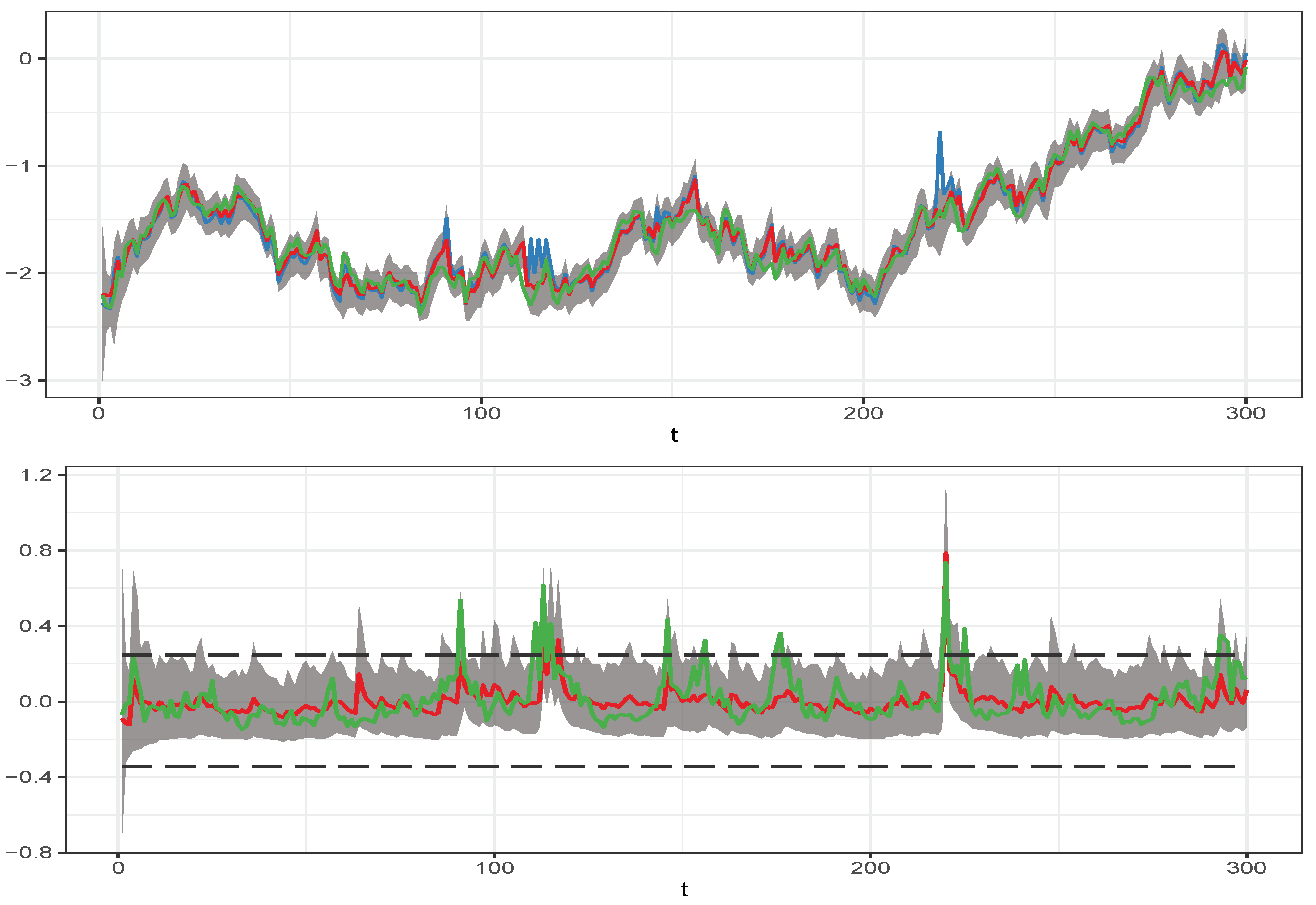
In order to illustrate the capability of our Bayesian storage SSM approach to empirically separate the variation in the observed prices into the variation generated by the structural storage model component and that of the stochastic trend, we conducted a simulation experiment. Prices were simulated from the storage SSM for parameters that were set equal to their posterior mean values found for the empirical application to natural gas prices, discussed further below (see Table 1). Prices were simulated for 800 periods, with the first 500 discarded as burn-in, so that the size of the simulated sample was . The storage SSM was then fit to the time series of simulated prices by using the PMMH procedure, and the BPF was applied to produce estimates of the filtered mean for the storage model price component and the stochastic trend , evaluated at the posterior mean of the parameters.
Figure 1 shows the results of the simulation experiment. The upper panel displays the time series of the simulated log price and the actual simulated stochastic trend component together with the estimate of its filtered mean, and the lower panel shows the time series of the actual price component, which is generated by the competitive storage model together with its estimated filtered mean. Plotted also are the boundaries of the storage regimes. The values of the price component above the upper boundary correspond to the stock-out pricing regime, and the values below the lower boundary correspond to the full storage capacity pricing regime. The plotted time series showed that the estimated filtered means of the two price components track the time evolution of the true components quite well. We also observed that the estimated filtered means predicted most of the stock-out events, which is critically important for identifying the structural parameters of the storage model. These simulation results illustrate that our approach appears to be well capable of empirically identifying—from observed commodity prices—the fraction of the price variation that is due competitive storage decisions and to separate it from stochastic trend variation.
5. Empirical Application
In this section, we apply our Bayesian storage SSM approach to a historical monthly price dataset for the following four commodities: coffee (coffee, other mild Arabicas, New York cash price, ex-dock New York, U.S. cents per pound), cotton (average spot price in U.S. cents per pound for upland cotton—color 41, Leaf 4, Staple 34), aluminum (aluminum, London Metal Exchange (LME), unalloyed primary ingots, high-grade, minimum 99.7% purity, USD per metric ton), and natural gas (natural gas (U.S.), spot price at Henry Hub, Louisiana, USD per MBtu). The respective sample periods ranged from January 1989 until December 2018 () for coffee, cotton, and aluminum and from January 1997 until December 2018 () for natural gas. All prices are in nominal terms. The datasets were obtained from the Commodity Research Bureau and are available (along with code) in the supplementary material at https://github.com/kjartako/Storage-model, accessed on 1 November 2021. We used monthly instead of annual prices to allow for more information about short-term price movements, as well as to avoid potentially spurious averaging effects of annual prices (Guerra et al. 2015).
5.1. Estimation Results for the Storage SSM with a Stochastic Trend
For the Bayesian posterior analysis of the storage SSM, we ran the PMMH algorithm for 12,000 iterations and discard the first 2000 as burn-in. In order to evaluate the sampling efficiency of the PMMH for estimating the parameters, we computed the Effective Sample Size (ESS) of their posterior PMMH samples (Geyer 1992). The ESS measures the size of a hypothetical independent sample directly drawn from the posterior of the parameters, which delivers the same numerical precision as the actual sample of M correlated PMMH parameter draws, so that large ESS values are to be preferred.
Table 1 summarizes the results of the Bayesian analysis of the storage SSM for the marginal likelihood preferred value of the capacity limit C. It provides the estimated posterior mean, standard deviation, and ESS for the parameters together with the preferred value for C for each of the four commodities. (The log marginal likelihood for the complete set of selected grid values of C obtained for the four commodities is given in Appendix C.) The results in Table 1 reveal that the marginal likelihood selects a significantly lower storage capacity limit C for natural gas than for the other three commodities. The selected capacity limits that we found are at the lower (natural gas) or upper bound (coffee, cotton, aluminum) of the considered range of grid values for C. The results of a further reduction of C for natural gas or a further increase of C for coffee, cotton, and aluminum (not reported here) showed no further significant improvements in the marginal likelihood that went beyond the numerical estimation error of their MCMC estimate. The ESS values ranged from 515 to 1188, indicating a satisfactory sampling efficiency with a fairly fast mixing rate of the PMMH algorithm. The estimates for the standard deviation of the trend innovations v imply that the stochastic trend accounts for 53% of the variation observed in the monthly price changes for natural gas, 58% for coffee, 65% for cotton, and 71% for aluminum. As for the estimates of the depreciation rate , we observed that they were fully in line with the actual storage costs to be expected for the different types of commodities: For natural gas, we found the largest estimated depreciation rate (1.1%), which implies that the monthly cost of storage amounts to 1.5% of the price. This relatively large estimated storage cost is in accordance with the fairly expensive storage technology for U.S. natural gas, which is typically stored in underground salt caves and similar facilities. The second largest storage cost was found for coffee, with a monthly depreciation rate of 0.3%, leading to estimated monthly costs of 0.7% of the price. The lowest storage costs were predicted for the nonfood and nonenergy products cotton and aluminum, for which the estimated depreciation rate ranged from 0.1% to 0.2%, resulting in storage costs of 0.5% for aluminum and 0.6% for cotton. We also observed that the larger the estimated storage cost for a commodity, the larger the fraction of observed price variation was, which was captured by the storage decision behavior. This is in agreement with the rationality of the competitive storage model, where higher storage costs are associated with more frequent stock-out events, which in turn implies greater price volatility. The posterior mean values for the slope parameter b of the inverse demand function imply that a reduction in supply on the market by one standard deviation of production leads to a price increase of 42% for natural gas, 148% for coffee, 130% for cotton, and 103% for aluminum. Therefore, the demand for natural gas is much more elastic with regard to price changes than the demand for the other three commodities, suggesting that the gas market is less prone to large price peaks. From the economic point of view, this is consistent with our result that the storage capacity C identified for natural gas is the smallest of all commodities, since the smaller the price peaks, the less valuable storage becomes, which makes large storage capacities less profitable.
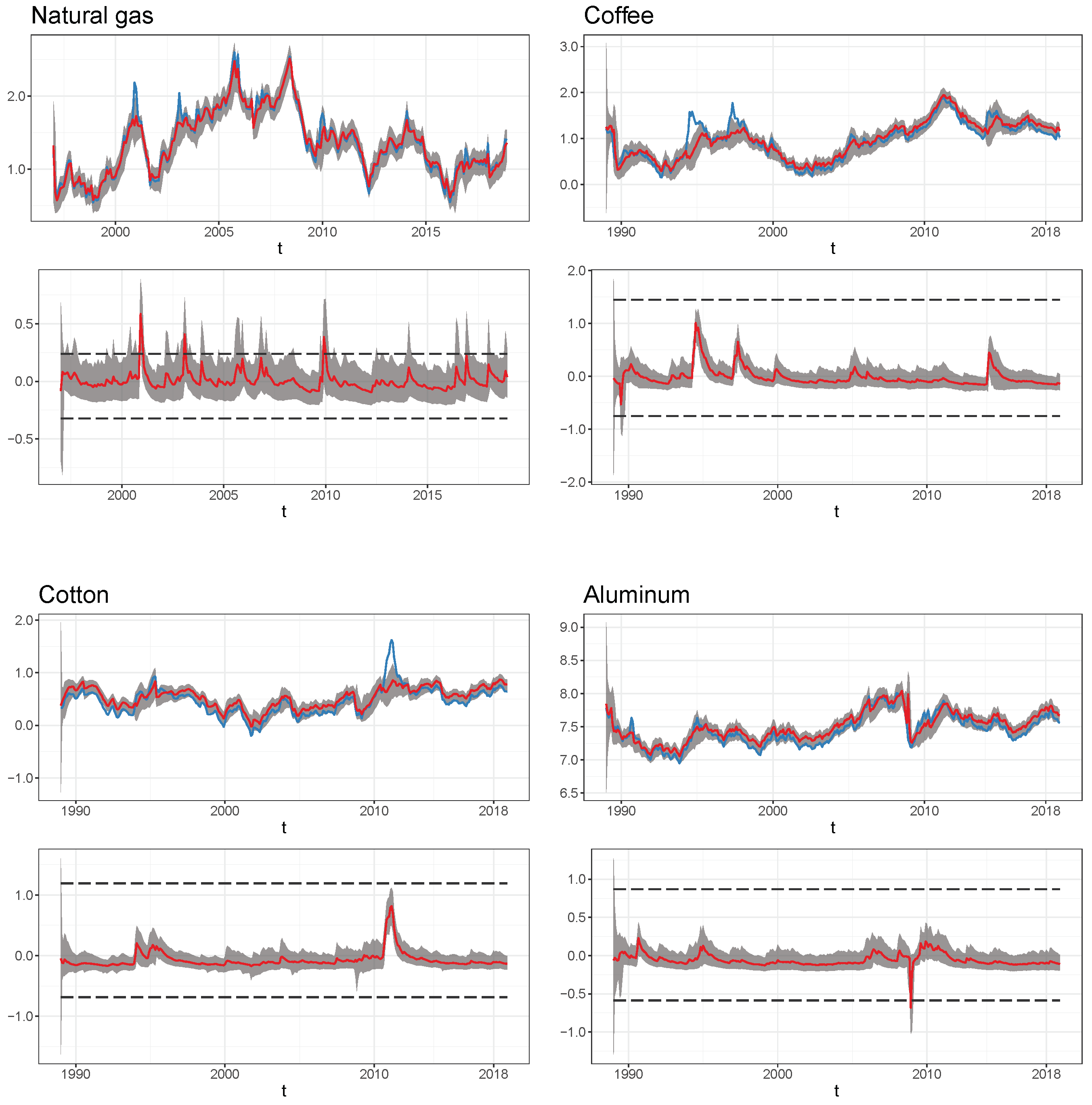
Figure 2 displays the time series of the log-prices for each of the four commodities, together with the filtered mean for their stochastic trend component and their price component associated with the competitive storage model . We observed that the temporal evolution of the filtered estimates of the stochastic trend variable closely followed that of the observed prices. The filtered estimates for the storage model price component revealed that it predominantly captures periodically recurring price fluctuations with large price peaks and drops. Beyond the periods with elevated price volatility, the contribution of this component to the price variation appears small. This reflects that when equilibrium storage is an inner solution (so that ), the resulting price is subject to an intertemporal price restriction, leading to prices that behave as a stationary Markov process. Accordingly, in this no-arbitrage pricing regime, the economic storage model provides little additional information about the price evolution that goes beyond the stochastic trend. However, storage becomes empirically relevant with a significant impact on the price behavior when the normal no-arbitrage pricing mechanism collapses in the stock-out and full-capacity regime, or is close to reaching these regimes. This occurs in the storage model in periods of severe and prolonged commodity shortages or oversupply.
The limits-to-arbitrage regimes (stock-out or full-capacity) identified by the SSM model and the periods with prices close to these regimes usually coincide with known historical market events. For example, the time periods with peaks in the filtered storage price component for natural gas usually correspond to periods when the historical level of natural gas storage in the market was very low (Kleppe and Oglend 2017). The sharp drop in the storage price component for aluminum in 2008–2009 is in line with the sharp decline in global aluminum demand, which in this period after the subprime crisis resulted in a large stock overhang. The coffee price drop in 1989 coincides with the collapse of the International Coffee Agreement (a cartel of coffee-producing countries) and oversupply in the market due to World Bank subsidies, while the 1994 peak is consistent with a negative supply shock triggered by significant frost damage in much of the coffee-growing areas of Brazil. The cotton price peak detected by the storage model in 2011 was arguably due to the severe global shortages, which were caused, inter alia, by the tightening of Indian export restrictions on cotton. However, under the fitted model for coffee and cotton with its relatively large estimated value for the storage capacity C, the peaks and drops in the estimated filtered mean of the storage price component are within the limits of the no-arbitrage pricing.
5.2. Model Comparisons
In this section, we assess the empirical relevance of the price component related to the competitive storage model to explain the observed price variation and compare the storage SSM model with stochastic trend to that with deterministic trend specifications. For this assessment, we relied on the marginal likelihood, as well as diagnostic checks on the Pearson and PIT residuals.
5.2.1. Alternative Models
To assess the relevance of the storage model price component, we compared our SSM model to the restricted SSM that results in the absence of storage. The latter was obtained by letting , making storage prohibitively costly, so that the stock process collapses to that of the supply shocks . In this case, the SSM in Equations (1)–(3) with the assumed inverse demand function reduces to:
This represents a standard linear Gaussian Local Level (LGLL) SSM (Durbin and Koopman 2012) so that the Kalman filter can be applied for likelihood evaluation. As the Kalman filter provides exact values for the likelihood, the PMMH used for simulating from the posterior of the parameters for the unrestricted storage SSM can be replaced by a standard MH algorithm. The priors assigned to the two parameters are the same as those we assumed for the unrestricted storage SSM.
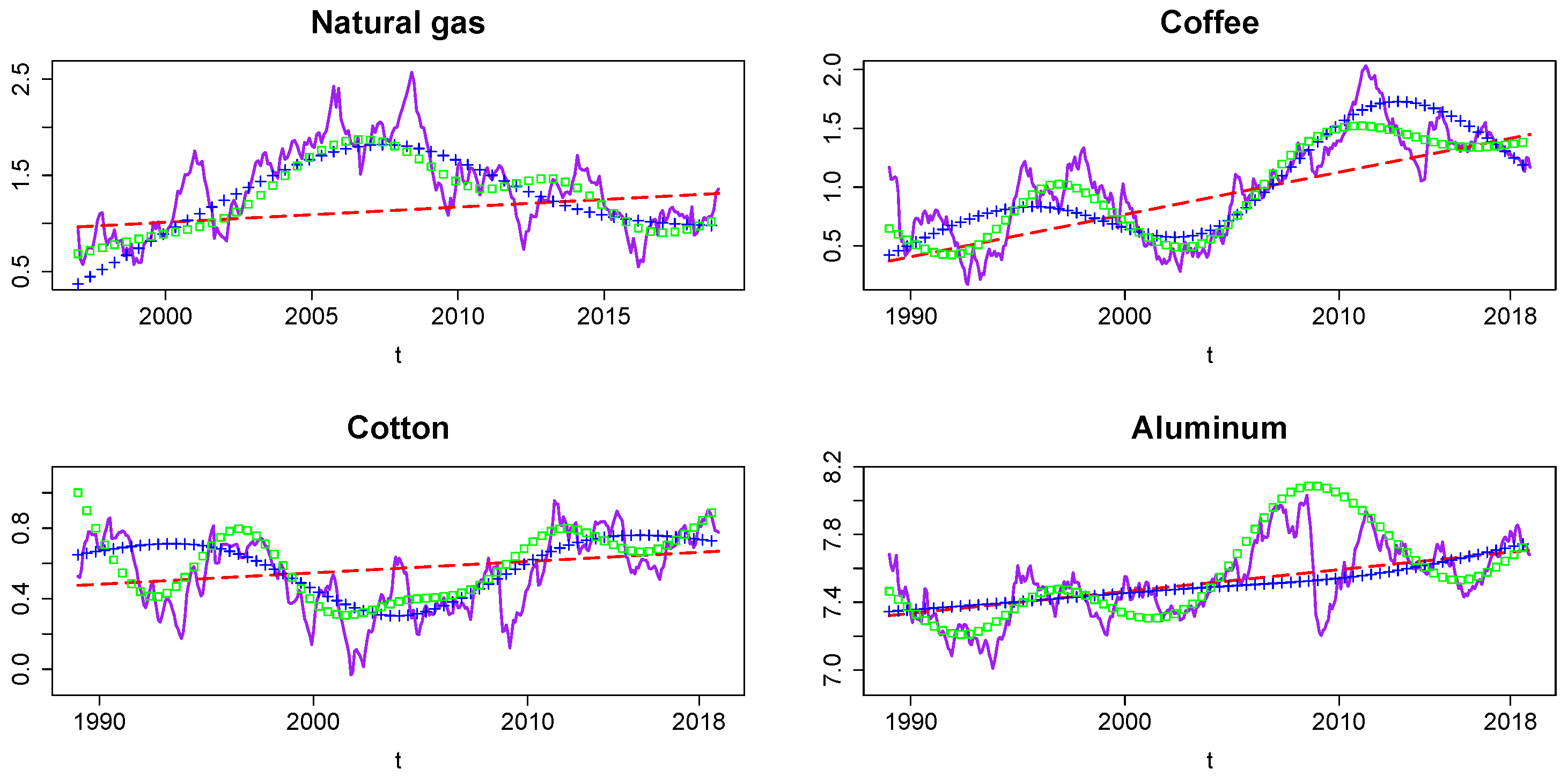
As deterministic trend specifications to be compared with the stochastic trend in the storage SSM, we considered those used in the study of Gouel and Legrand (2017). They used a linear time trend, for which in Equation (2) is replaced by . In addition, they considered restricted cubic spline trend specifications of the form , where are the basis functions of B-splines, G are the degrees of freedom, and are the corresponding trend parameters to be estimated. For our comparison, we considered restricted cubic splines with three knots (RCS3) and five trend parameters, as well as seven knots (RCS7) and nine trend parameters1. For these deterministic trends, the SSM in Equations (1)–(3) reduces to a univariate, nonlinear autoregression for the log-price:
Analogous to the LGLL SSM, we can simulate from the posterior for the parameters of the deterministic trend models by using a standard MH algorithm. To select C, we used the same grid search based on the marginal likelihood as for the storage SSM and assumed the same priors for the structural parameters . We assigned independent priors to the deterministic trend parameters . The estimates of the structural parameters for the deterministic trend models are found in Appendix C. For details on the computation and derivation of the Pearson and PIT residuals of the deterministic trend models, see Appendix B.3.
5.2.2. Marginal Likelihood Model Comparisons and Diagnostics Checks
Table 2 provides the log-marginal likelihood values for the storage SSM together with those of the LGLL SSM and the storage model combined with the deterministic trend specifications for the C values that were selected by the marginal likelihood. Reported also are the resulting values for the log-Bayes factor of the storage SSM relative to the four alternative models . The results reveal that the storage SSM is strongly preferred over the LGLL SSM for all commodities, which suggests that the structural storage component in the SSM substantially contributes to the model fit. Hence, the nonlinear price dynamics with periodically recurring increases in price volatility and price spiking, as predicted by the competitive storage model, adds significantly to explaining the price behavior. For all commodities, we also observed that the storage SSM is clearly favored over all deterministic trend specifications. Thus, the storage SSM has a trend component that is not only consistent with the rationality of the economic model, but is also much more supported by the data than the deterministic trends, such as those used by Gouel and Legrand (2017) for the estimation of the structural parameters of the competitive storage model. Our estimates of the structural parameters for the deterministic trend models are found in Appendix C. Figure 3 shows the time series plots of the fitted deterministic trends and the smoothed mean of the stochastic trend , all computed by setting the parameters to their posterior mean values2. Unsurprisingly, we found that the stochastic trend typically captures a substantially larger fraction of the observed price variations than the deterministic trends.
Table 3 provides the results of diagnostic checks on the PIT residuals and the Pearson residuals for the storage SSM and the four alternative models considered. The PIT residuals of the storage SSM suggest that this model captures well the observed distributional properties of the commodity prices, with the exception of the price for coffee. The skewness and kurtosis of the PIT residuals of the storage SSM for the other three commodities are close to their benchmark values for a normal distribution, and they passed the Jarque–Bera normality test at the 1% significance level. In contrast, the LGLL SSM, as well as the storage models with deterministic trends typically have more difficulties approximating the distributional properties of the prices. Only the PIT residuals of the storage model with an RCS7 trend for aluminum passed the Jarque–Bera normality test at a conventional significance level.
The first-order serial correlation of the Pearson residuals and the p-values of the Ljung–Box test for and including 12 lags reported in Table 3 show the following: The storage SSM is able to explain the observed autocorrelation in the level and volatility of the gas price and the volatility of the coffee price, while in all other cases, there is significant residual autocorrelation. However, in these cases, all competing models cannot fully capture the serial correlation either. Clearly, based on these results, we cannot identify whether the failure of the storage SSM and the deterministic trend models to explain all of the observed dynamics in the coffee, cotton, and aluminum prices is due to a potential misspecification of the trend or the competitive storage model itself, since the diagnostic tests are—as any specification test in this context—joint tests for the validity of both price components.
In sum, the results showed that the storage SSM generally outperforms the deterministic trend models in explaining the observed distributional properties of commodity prices and that its ability to account for the dynamics in the price levels is not worse.
5.2.3. Estimates for Annual Storage Costs and Price Elasticity of Demand
As is evident from Figure 3, trends differ substantially across the different trend specifications. Because of this, the dynamic and distributional characteristics of detrended prices will also differ substantially depending on whether a stochastic or deterministic trend is assumed. Therefore, it can be expected that the nature of the trend has a critical impact on the estimates of the parameters that determine the storage costs () and the price elasticity of demand (b), since these parameters are identified by the strength of the serial correlation and the size of the spikes in the trend-adjusted prices. The lower the storage costs in the competitive storage model are, the stronger the predicted serial correlation, while the more inelastic the demand is, the larger the resulting price spikes. As larger price spikes also imply more speculative storage activity, an inelastic demand also contributes to the strength of the predicted serial correlation in the prices.
Table 4 summarizes the estimates for the annualized storage costs (net of interest costs) in percent of the average price and the price elasticities of demand obtained from the fitted storage SSM and the deterministic trend models. The annual storage costs are computed as , and the price elasticity is given by , where is the mean supply. We observed that the estimated storage costs for gas and coffee under the SSM with stochastic trend are slightly higher than under the respective deterministic trend model, which is preferred by the marginal likelihood, and substantially smaller for cotton and aluminum. We also found that the SSM with stochastic trend predicts more elastic demands for all commodities, but especially for gas, than the deterministic trend models. The larger elasticities found under the storage SSM reflect that the stochastic trend produces, due to its greater flexibility to track the observed price, trend-adjusted prices that have spikes that are smaller than those obtained under a deterministic trend. Hence, in contrast to the deterministic trend specifications, the stochastic trend SSM is not forced to match the large spikes observed in the actual prices by imposing less elastic demands. For natural gas, the residual serial correlation in the prices adjusted by the stochastic trend component also appears to be relatively low, which indicates relatively high storage costs. However, for the other commodities, this residual serial correlation is larger, leading to substantially lower estimated storage costs.
Gouel and Legrand (2017) provided estimates of storage costs and price elasticities of demand based on deterministic trend models used for annual data on various commodities, including coffee and cotton. This allows for some comparisons with our results for those two commodities. The annual storage costs estimates they reported for their preferred trend model for coffee and cotton were, respectively, 1.4% and 0.3% of the average price. These estimates based on annual data are much lower than those we found for the storage SSM, as well as the deterministic trend models fitted to monthly data. However, they argued that their estimated annual costs are possibly too small—an assessment that is consistent with our estimates for the storage costs. For the annual price elasticity of demand, the estimates of Gouel and Legrand (2017) were −0.04% for coffee and −0.03% for cotton. These estimates imply less elastic demands for these commodities than our estimates based on the storage SSM. One can argue which elasticities better reflect the markets. Mehta and Chavas (2008) assumed a range of plausible values for the annual elasticity of demand for coffee between −0.2% and −0.4%, while Duffy et al. (1990) argued that the annual export demand for cotton is likely fairly elastic. Our elasticity estimates therefore agree somewhat better with these assessments than those of Gouel and Legrand (2017). However, they are well below the range of plausible values found by Mehta and Chavas (2008).
6. Conclusions
In this paper, we proposed a stochastic trend competitive storage model for commodity prices, which defines a nonlinear State-Space Model (SSM). For the Bayesian posterior analysis of the proposed stochastic trend SSM, we used an efficient MCMC procedure. This adds to existing empirical commodity storage models based on deterministic trend specifications. Our stochastic trend approach fits into the economic rationality of the competitive storage model and is also sufficiently flexible to account for the variation in the observed prices that the competitive storage model is not intended to explain. The obvious benefit is that it makes the storage model applicable to markets with highly persistent unit root-like prices, which appears relevant for many commodity markets. Our approach aims at increasing the empirical relevance and applicability of the competitive storage model.
The MCMC procedure we proposed for jointly estimating the structural and trend parameters in the SSM is a particle marginal Metropolis–Hastings algorithm based on the bootstrap particle filter. A Monte Carlo simulation experiment showed that this approach is able to disentangle the stochastic trend from the price variation due to speculative storage. The SSM was applied to monthly price data for natural gas, cotton, coffee, and aluminum. Not surprisingly, the stochastic trend explains a large part of the observed variation in the commodity prices. More importantly, the competitive storage component adds short-run price volatility and price spiking and becomes periodically relevant to explain nonlinear pricing behavior related to states of market turmoil. A formal empirical comparison of the SSM to the corresponding model that resulted in the absence of storage suggests that the speculative storage price component significantly contributes to commodity price variation.
Which trend to apply will depend on the specific market under consideration. If a stochastic trend is not appropriate, fitting a highly flexible stochastic trend model risks overfitting the price variation and downplaying the contribution of the storage model. Consequently, the price elasticity of demand will tend to be overestimated and the estimates of the storage costs can be expected to be correspondingly biased. On the other hand, failing to account for a stochastic trend when it is appropriate will tend to underestimate the elasticity of demand. Our empirical results showed that the stochastic trend model typically estimates a higher elasticity of demand and a different amount of storage costs than existing deterministic trend models for the commodity markets investigated in this paper. Pretesting of price characteristics can guide trend choice. For instance, unit root tests can be applied to evaluate whether a stochastic trend specification is suitable.
The empirical comparison of the stochastic trend SSM to existing deterministic trend models using the Bayes factor and diagnostic tests showed that, all in all, the stochastic trend performs favorably in relation to the deterministic trend specifications. In particular, the stochastic SSM captures the observed distributional properties of prices (i.e., skewness and kurtosis) better than the deterministic trend models, but does not fully explain them for the coffee price. While the stochastic trend SSM also accounts for the price dynamics in the observed prices on the natural gas market, it is not able to fully capture all the serial dependence of the coffee, cotton, and aluminum prices. This is similar to the results of financial approaches on modeling commodity term structures, showing the relevance of additional pricing factors beyond the traditional ones for the spot price and the convenience yield (Miltersen and Schwartz 1998; Schwartz 1997; Tang 2012). The stochastic trend SSM is essentially a two-factor model with one reduced-form random walk component orthogonally appended to a factor restricted by economic constraints. Increasing the flexibility in the economic model will arguably improve the explanatory power of the model, although with additional statistical challenges in separately identifying the trend behavior from the price component related to the competitive storage model.
Supplementary Materials
All code is available at https://github.com/kjartako/Storage-model, accessed on 1 November 2021.
Author Contributions
Conceptualization, K.K.O., T.S.K., R.L. and A.O.; methodology, K.K.O., T.S.K., R.L. and A.O.; software, K.K.O. and T.S.K.; validation, K.K.O., T.S.K., R.L. and A.O.; writing—original draft preparation, K.K.O., T.S.K., R.L. and A.O.; writing—review and editing, K.K.O., T.S.K., R.L. and A.O.; visualization, K.K.O. All authors have read and agreed to the published version of the manuscript.
Funding
This research received no external funding.
Institutional Review Board Statement
Not applicable.
Informed Consent Statement
Not applicable.
Data Availability Statement
The data are available in the supplementary material at https://github.com/kjartako/Storage-model, accessed on 1 November 2021.
Acknowledgments
The authors thank the three anonymous reviewers for their helpful suggestions and comments.
Conflicts of Interest
The authors declare no conflict of interest.
Appendix A. Numerical Solution of the Price Function
The numerical algorithm we use to solve the functional equation for the price function as defined by Equations (4)–(6) is based on that used by Kleppe and Oglend (2019) for a model with autocorrelated supply shocks. The algorithm is based on solving the storage policy function and then recover via Equation (6), which implies that:
Let be defined such that and such that . For , so that , it follows that (stock-out regime); for , so that , it follows that (storage regime); and for , so that , it follows that (full capacity storage regime).
The numerical representation of is given by , where the function (with for ) is represented on a (comparatively sparse) grid on and is evaluated using a suitable interpolation method (e.g., linear). The resulting approximation is given by:
and correspondingly .
The iteration to find consists of the following steps:
- Select an initial guess, e.g., , where is the linear function such that , . Set ;
- Update the left kink point according to:
- Update the right kink point according to:
- Update the grid to be on
- For each grid point j, find the update as the solution in s to:using a univariate nonlinear root-finding algorithm. Notice that the solution is constrained to be in and that , ;
- Until convergence, set and go back to Step 2.
The integrals in Equations (A2)–(A4) are approximated using the trapezoidal quadrature rule with 128 subintervals, over the interval , and the nonlinear Equation (A4) is solved using Brent’s method. Allowing the grid space to adjust to the updated functional solutions ensures that the grid can dynamically concentrate in the region of the state-space where a high precision is needed, namely the region defining the storage regime. This provides both efficient and precise numerical solutions to the pricing function.
Appendix B. Computational Details for Statistical Inference
Appendix B.1. Particle Filter
Here we outline the implementation of the BPF of Gordon et al. (1993) that we use to approximate the likelihood in the Bayesian PMMH analysis of the storage SSM and to predict (functions of) the latent states required to compute diagnostic statistics.
For given values of the parameters , the BPF produces MC estimates for the sequence of period-t likelihood contributions by sequentially sampling and resampling values of the latent states (particles) using the state-transition density as importance sampling density. For implementation we rely on a dynamic resampling scheme in which the particles are resampled only when their effective sample size falls below one half of the number of particles (Doucet and Johansen 2009). This BPF for approximating the likelihood as given by Equations (10)–(12) consists of the following steps:
- For period (initialization): Sample for , and set the corresponding (normalized) IS weights to . For initialization, set ;
- For periods : Sample for , and set . Compute the IS weights as:and their normalized versions . Then use the IS weights to obtain the period-t likelihood contribution as , and compute the effective particle sample size defined by . If , resample from the particles with replacement according to their IS weights to obtain the resampled particles , and set their weights to . Otherwise, set .
The resulting BPF estimate for the likelihood (conditional on the first price observation) is given by .
In our applications, we use 10,000 particles. For a time series with , one BPF likelihood estimate requires approximately 2.5 s (on a computer with an Intel Core i5-6500 processor running at 3.20 GHz). The MC numerical standard deviation of the log-likelihood estimate , computed from reruns of the BPF for a fixed value under different seeds, is about 0.1 percent of the absolute value of the log-likelihood, illustrating the high accuracy of the BPF.
The BPF for MC likelihood approximation delivers as a by-product MC estimates for the conditional mean of functions given . This conditional mean (as reproduced from Equation (14)) is given by:
Since the particles and IS-weights produced by the BPF provide an MC approximation to this filtering density , the conditional mean in Equation (A6) for a given value of can be easily estimated by:
with , where is obtained by propagating the BPF particle via the state-transition density, i.e., .
Appendix B.2. Marginal Likelihood
In order to evaluate the marginal likelihood for the storage SSM we rely upon the procedure developed by Chib and Jeliazkov (2001) which is based on the output of a Bayesian MH posterior analysis. This procedure takes advantage of the fact that the marginal likelihood given in Equation (17) can be expressed as:
where is the likelihood function for the observed prices evaluated at some value of the parameters , and and are the corresponding ordinates of the prior and posterior of the parameters. Then it exploits that the posterior ordinate can be expressed in terms of the MH acceptance probability and the proposal density . Namely, as the ratio of the expectation of under the posterior relative to the expectation of under the proposal density . This implies that a consistent MC estimate for based on the MH acceptance probability defined in Equation (13) is given by:
where are the M simulated draws from the posterior distribution and are draws from the proposal distribution . For evaluating the likelihood in Equation (A8) we use the same BPF algorithm as applied for the likelihood evaluation in the MH acceptance probabilities in Equation (13) (and outlined in the previous subsection). The value of the point is set equal to the posterior mean of .
Appendix B.3. Residuals for the Deterministic Trend Models
For the deterministic trend models as given by Equation (18) the conditional expectation and variance defining the Pearson residuals in Equation (15) can be evaluated by MC integration as the sample mean and variance of the simulated prices:
where are iid draws from a distribution.
The PIT residuals in Equation (16) obtain as follows: The probability , which follows for a correctly specified model a uniform distribution on the unit interval, results as:
where . Equation (A12) follows from the fact that the inverse of the rational expectations equilibrium price function is monotonically non-increasing. Since is a random variate with cdf denoted by , Equation (A13) implies that . Since for it holds that , the PIT residuals are given by:
Appendix C. Additional Results
Table A1 reports the log marginal likelihood for the grid values of the storage capacity limit C obtained for the four commodities.

Table A1.
Log marginal likelihood of the storage SSM for .
| C | Natgas | Coffee | Cotton | Aluminum |
|---|---|---|---|---|
| 10 | 164.13 | 420.07 | 522.80 | 545.36 |
| 15 | 163.89 | 425.93 | 530.93 | 549.77 |
| 20 | 163.68 | 429.32 | 536.81 | 553.16 |
| 25 | 163.57 | 431.10 | 539.89 | 555.41 |
Table A2 provides the posterior mean and standard deviation for the structural parameters of the competitive storage model combined with deterministic trend specifications under the marginal-likelihood preferred value for the capacity limit C (see Table 2).
Table A2.
Estimates for the storage model parameters under the storage model with deterministic trends.
Table A2.
Estimates for the storage model parameters under the storage model with deterministic trends.
| Natgas | Coffee | Cotton | Aluminum | |||
|---|---|---|---|---|---|---|
| Linear | Post. mean | 0.0110 | 0.0041 | 0.0009 | 0.0046 | |
| Post. std. | 0.0051 | 0.0049 | 0.0007 | 0.0026 | ||
| RCS3 | Post. mean | 0.0073 | 0.0023 | 0.0009 | 0.0037 | |
| Post. std. | 0.0040 | 0.0014 | 0.0007 | 0.0021 | ||
| RCS7 | Post. mean | 0.0087 | 0.0055 | 0.0034 | 0.0015 | |
| Post. std. | 0.0080 | 0.0021 | 0.0007 | 0.0010 | ||
| b | Linear | Post. mean | 4.85 | 4.18 | 3.56 | 2.09 |
| Post. std. | 0.200 | 0.282 | 0.153 | 0.106 | ||
| RCS3 | Post. mean | 3.18 | 4.37 | 3.62 | 3.25 | |
| Post. std. | 0.164 | 0.190 | 0.154 | 0.172 | ||
| RCS7 | Post. mean | 5.99 | 4.04 | 3.64 | 2.11 | |
| Post. std. | 0.920 | 0.316 | 0.163 | 0.095 |
| 1 | The knots for the RCS3 specification are located at the 25%, 50%, and 75% quantiles of the time index and for the RCS7 at the 12.5%, 25%, 37.5%, 50%, 67.5%, 75%, and 87.5% quantiles. |
| 2 | The smoothed mean was computed using the particle smoothing algorithm, which adds to the BPF, as outlined in Appendix B.1, a backward sampling step (Doucet and Johansen 2009, Section 5). |
References
- Andrieu, Christophe, Arnaud Doucet, and Roman Holenstein. 2010. Particle markov chain monte carlo methods. Journal of the Royal Statistical Society: Series B (Statistical Methodology) 72: 269–342. [Google Scholar] [CrossRef] [Green Version]
- Bobenrieth, Eugenio, Brian Wright, and Di Zeng. 2013. Stocks-to-use ratios and prices as indicators of vulnerability to spikes in global cereal markets. Agricultural Economics 44: 43–52. [Google Scholar] [CrossRef] [Green Version]
- Bos, Charles S., and Neil Shephard. 2006. Inference for adaptive time series models: Stochastic volatility and conditionally gaussian state space form. Econometric Reviews 25: 219–44. [Google Scholar] [CrossRef] [Green Version]
- Cafiero, Carlo, Eugenio Bobenrieth, and Juan Bobenrieth. 2011. Storage arbitrage and commodity price volatility. In Safeguarding Food Security in Volatile Global Markets. Rome: Food and Agriculture Organization of the United Nations (FAO), pp. 288–326. [Google Scholar]
- Cafiero, Carlo, Eugenio Bobenrieth, Juan Bobenrieth, and Brian D. Wright. 2011. The empirical relevance of the competitive storage model. Journal of Econometrics 162: 44–54. [Google Scholar] [CrossRef] [Green Version]
- Cafiero, Carlo, Eugenio Bobenrieth, Juan Bobenrieth, and Brian D. Wright. 2015. Maximum likelihood estimation of the standard commodity storage model: Evidence from sugar prices. American Journal of Agricultural Economics 97: 122–36. [Google Scholar] [CrossRef]
- Canova, Fabio. 2014. Bridging dsge models and the raw data. Journal of Monetary Economics 67: 1–15. [Google Scholar] [CrossRef] [Green Version]
- Cappé, Olivier, Simon J. Godsill, and Eric Moulines. 2007. An overview of existing methods and recent advances in sequential monte carlo. Proceedings of the IEEE 95: 899–924. [Google Scholar] [CrossRef]
- Chib, Siddhartha, and Ivan Jeliazkov. 2001. Marginal likelihood from the Metropolis-Hastings output. Journal of the American Statistical Association 96: 270–81. [Google Scholar] [CrossRef] [Green Version]
- Deaton, Angus, and Guy Laroque. 1992. On the behaviour of commodity prices. The Review of Economic Studies 59: 1–23. [Google Scholar] [CrossRef] [Green Version]
- Deaton, Angus, and Guy Laroque. 1995. Estimating a nonlinear rational expectations commodity price model with unobservable state variables. Journal of Applied Econometrics 10: S9–S40. [Google Scholar] [CrossRef]
- Deaton, Angus, and Guy Laroque. 1996. Competitive Storage and Commodity Price Dynamics. The Journal of Political Economy 104: 896–923. [Google Scholar] [CrossRef] [Green Version]
- DeJong, David N., and Chetan Dave. 2011. Structural Macroeconometrics, 2nd ed. Princeton: Princeton University Press. [Google Scholar]
- Doucet, Arnaud, and Adam M. Johansen. 2009. A tutorial on particle filtering and smoothing: Fifteen years later. In The Oxford Handbook of Nonlinear Filtering. Oxford: Oxford University Press, pp. 656–704. [Google Scholar]
- Duffy, Patricia A., Michael K. Wohlgenant, and James W. Richardson. 1990. The elasticity of export demand for us cotton. American Journal of Agricultural Economics 72: 468–74. [Google Scholar] [CrossRef]
- Durbin, James, and Siem Jan Koopman. 2012. Time Series Analysis by State Space Methods, 2nd ed. Number 38 in Oxford Statistical Science. Oxford: Oxford University Press. [Google Scholar]
- Flury, Thomas, and Neil Shephard. 2011. Bayesian inference based only on simulated likelihood: Particle filter analysis of dynamic economic models. Econometric Theory 27: 933–56. [Google Scholar] [CrossRef] [Green Version]
- Geyer, Charles J. 1992. Practical Markov chain Monte Carlo. Statistical Science 7: 473–83. [Google Scholar] [CrossRef]
- Gordon, Neil J., David J. Salmond, and Adrian F. M. Smith. 1993. Novel approach to nonlinear/non-gaussian bayesian state estimation. IEE Proceedings F-Radar and Signal Processing 140: 107–113. [Google Scholar] [CrossRef] [Green Version]
- Gouel, Christophe, and Nicolas Legrand. 2017. Estimating the competitive storage model with trending commodity prices. Journal of Applied Econometrics 32: 744–63. [Google Scholar] [CrossRef] [Green Version]
- Guerra, Ernesto A., Eugenio S. A. Bobenrieth, Juan R. A. Bobenrieth, and Carlo Cafiero. 2015. Empirical commodity storage model: The challenge of matching data and theory. European Review of Agricultural Economics 42: 607–23. [Google Scholar] [CrossRef] [Green Version]
- Gustafson, Robert L. 1958. Carryover Levels for Grains: A Method for Determining Amounts That Are Optimal under Specified Conditions; Number 1178; Washington: US Department of Agriculture.
- Haario, Heikki, Eero Saksman, and Johanna Tamminen. 2001. An adaptive Metropolis algorithm. Bernoulli 7: 223–42. [Google Scholar] [CrossRef] [Green Version]
- Kim, Sangjoon, Neil Shephard, and Siddhartha Chib. 1998. Stochastic volatility: Likelihood inference and comparison with arch models. The Review of Economic Studies 65: 361–93. [Google Scholar] [CrossRef]
- Kleppe, Tore Selland, and Atle Oglend. 2017. Estimating the competitive storage model: A simulated likelihood approach. Econometrics and Statistics 4: 39–56. [Google Scholar] [CrossRef] [Green Version]
- Kleppe, Tore Selland, and Atle Oglend. 2019. Can limits-to-arbitrage from bounded storage improve commodity term-structure modeling? Journal of Futures Markets 39: 865–89. [Google Scholar] [CrossRef]
- Koop, Gary, and Dimitris Korobilis. 2013. Large time-varying parameter vars. Journal of Econometrics 177: 185–98. [Google Scholar] [CrossRef] [Green Version]
- Legrand, Nicolas. 2019. The empirical merit of structural explanations of commodity price volatility: Review and perspectives. Journal of Economic Surveys 33: 639–64. [Google Scholar] [CrossRef]
- Liesenfeld, Roman, and Jean-François Richard. 2003. Univariate and multivariate stochastic volatility models: Estimation and diagnostics. Journal of Empirical Finance 10: 505–31. [Google Scholar] [CrossRef]
- Mehta, Aashish, and Jean-Paul Chavas. 2008. Responding to the coffee crisis: What can we learn from price dynamics? Journal of Development Economics 85: 282–311. [Google Scholar] [CrossRef] [Green Version]
- Miltersen, Kristian R., and Eduardo S. Schwartz. 1998. Pricing of options on commodity futures with stochastic term structures of convenience yields and interest rates. Journal of Financial and Quantitative Analysis 33: 33–59. [Google Scholar] [CrossRef]
- Oglend, Atle, and Tore Selland Kleppe. 2017. On the behavior of commodity prices when speculative storage is bounded. Journal of Economic Dynamics and Control 75: 52–69. [Google Scholar] [CrossRef]
- Richard, Jean-François, and Wei Zhang. 2007. Efficient high-dimensional importance sampling. Journal of Econometrics 127: 1385–411. [Google Scholar] [CrossRef] [Green Version]
- Routledge, Bryan R., Duane J. Seppi, and Chester S. Spatt. 2000. Equilibrium forward curves for commodities. The Journal of Finance 55: 1297–337. [Google Scholar] [CrossRef] [Green Version]
- Sala, Luca. 2015. Dsge models in the frequency domains. Journal of Applied Econometrics 30: 219–40. [Google Scholar] [CrossRef]
- Schwartz, Eduardo S. 1997. The stochastic behavior of commodity prices: Implications for valuation and hedging. The Journal of Finance 52: 923–73. [Google Scholar] [CrossRef]
- Shephard, Neil, and Michael K. Pitt. 1997. Likelihood analysis of non-Gaussian measurement time series. Biometrika 84: 653–67. [Google Scholar] [CrossRef]
- Tang, Ke. 2012. Time-varying long-run mean of commodity prices and the modeling of futures term structures. Quantitative Finance 12: 781–90. [Google Scholar] [CrossRef] [Green Version]
- Wang, Dabin, and William G. Tomek. 2007. Commodity prices and unit root tests. American Journal of Agricultural Economics 89: 873–89. [Google Scholar] [CrossRef]
Figure 1.
Filtered price components for simulated data. Upper panel: time series plot of the simulated log price (blue line), the actual stochastic trend component (green line), and its estimated filtered mean (red line). Lower panel: time series plot of the actual storage model component (green line) and its estimated filtered mean (red line). The gray shaded areas indicate the 95% credible intervals under the filtering densities for and , and the black horizontal lines in the lower panel mark the boundaries of the storage regimes. The prices were simulated using parameters set at and . The posterior mean of the parameters obtained by fitting the model to the simulated price data are .

Figure 2.
Commodity prices and filtered price components. Upper panels: time series plot of the log price (blue line) and the estimated filtered mean of the stochastic trend component (red line). Lower panels: time series plot of the estimated filtered mean of the storage model component (red line). The gray shaded areas indicate the 95% credible intervals under the filtering densities for and , and the black horizontal lines in the lower panels mark the boundaries of the storage regimes. The parameters are set to their posterior mean as given in Table 1.

Figure 3.
Fit stochastic and deterministic trends. Smoothed stochastic trend (purple solid line), linear trend (red dashed line), RCS3 trend (blue plus sign), and RCS7 trend (green square).
Figure 3.
Fit stochastic and deterministic trends. Smoothed stochastic trend (purple solid line), linear trend (red dashed line), RCS3 trend (blue plus sign), and RCS7 trend (green square).

Table 1.
MCMC posterior analysis of the storage SSM with a stochastic trend. The reported numbers are the posterior mean, posterior standard deviation, and Effective Sample Size (ESS) for the parameters. The results are based on 12,000 PMMH iterations, discarding the first 2000 burn-in iterations.
Table 1.
MCMC posterior analysis of the storage SSM with a stochastic trend. The reported numbers are the posterior mean, posterior standard deviation, and Effective Sample Size (ESS) for the parameters. The results are based on 12,000 PMMH iterations, discarding the first 2000 burn-in iterations.
| Natgas | Coffee | Cotton | Aluminum | ||
|---|---|---|---|---|---|
| v | Post. mean | 0.0972 | 0.0574 | 0.0443 | 0.0422 |
| Post. std. | 0.0083 | 0.0034 | 0.0023 | 0.0022 | |
| ESS | 634 | 627 | 914 | 636 | |
| Post. mean | 0.0112 | 0.0025 | 0.0019 | 0.0014 | |
| Post. std. | 0.0048 | 0.0014 | 0.0010 | 0.0009 | |
| ESS | 580 | 544 | 708 | 770 | |
| b | Post. mean | 0.4196 | 1.4847 | 1.2969 | 1.0283 |
| Post. std. | 0.2594 | 0.4242 | 0.3080 | 0.3058 | |
| ESS | 515 | 741 | 1188 | 786 | |
| C | 10 | 25 | 25 | 25 |
Table 2.
Log-marginal likelihood values of the storage SSM and the alternative models. The log-Bayes factor of the storage SSM relative to the alternative models is in parentheses, and the marginal likelihood preferred values for C are in brackets.
Table 2.
Log-marginal likelihood values of the storage SSM and the alternative models. The log-Bayes factor of the storage SSM relative to the alternative models is in parentheses, and the marginal likelihood preferred values for C are in brackets.
| Natgas | Coffee | Cotton | Aluminum | |
|---|---|---|---|---|
| Storage SSM | 164.13 | 431.10 | 539.89 | 555.41 |
| [10] | [25] | [25] | [25] | |
| LGLL SSM | 146.76 | 404.09 | 510.28 | 540.88 |
| (17.37) | (27.01) | (29.61) | (14.53) | |
| Linear trend | 138.36 | 386.70 | 507.51 | 546.59 |
| [20] | [25] | [25] | [20] | |
| (25.77) | (44.40) | (32.38) | (8.82) | |
| RCS3 trend | 144.68 | 405.50 | 518.41 | 531.56 |
| [15] | [25] | [25] | [25] | |
| (19.45) | (25.60) | (21.48) | (23.85) | |
| RCS7 trend | 137.58 | 401.78 | 519.11 | 540.74 |
| [25] | [25] | [25] | [20] | |
| (26.55) | (29.32) | (20.78) | (14.67) |
Table 3.
Diagnostics on the PIT and Pearson residuals. Skewness, kurtosis, and p-value of the Jarque–Bera test (JB) for the PIT residuals. Lag-1 autocorrelation () and p-value of the Ljung–Box test (LB) for the Pearson residuals and their squared values, including 12 lags.
Table 3.
Diagnostics on the PIT and Pearson residuals. Skewness, kurtosis, and p-value of the Jarque–Bera test (JB) for the PIT residuals. Lag-1 autocorrelation () and p-value of the Ljung–Box test (LB) for the Pearson residuals and their squared values, including 12 lags.
| Skew (ξt) | Kurt (ξt) | JB (ξt) | ρ1 (ηt) | LB12 (ηt) | LB12 () | |
|---|---|---|---|---|---|---|
| Storage SSM | ||||||
| Natgas | 0.053 | 3.069 | 0.915 | 0.075 | 0.027 | 0.297 |
| Coffee | 0.452 | 4.050 | <0.001 | 0.224 | <0.001 | 0.452 |
| Cotton | −0.024 | 3.669 | 0.035 | 0.452 | <0.001 | <0.001 |
| Aluminum | −0.090 | 3.105 | 0.723 | 0.245 | <0.001 | <0.001 |
| LGLL SSM | ||||||
| Natgas | 0.033 | 4.298 | <0.001 | 0.084 | 0.055 | 0.452 |
| Coffee | 0.801 | 7.679 | <0.001 | 0.257 | <0.001 | <0.001 |
| Cotton | −0.230 | 6.325 | <0.001 | 0.502 | <0.001 | <0.001 |
| Aluminum | −0.381 | 4.652 | <0.001 | 0.268 | <0.001 | <0.001 |
| Linear trend | ||||||
| Natgas | 0.181 | 5.295 | <0.001 | 0.023 | 0.206 | 0.276 |
| Coffee | −0.680 | 5.736 | <0.001 | 0.246 | <0.001 | 0.095 |
| Cotton | −0.073 | 5.938 | <0.001 | 0.481 | <0.001 | <0.001 |
| Aluminum | 0.516 | 6.389 | <0.001 | 0.247 | <0.001 | <0.001 |
| RCS3 trend | ||||||
| Natgas | −0.109 | 4.022 | 0.003 | 0.014 | 0.002 | 0.031 |
| Coffee | −0.498 | 4.681 | <0.001 | 0.182 | <0.001 | 0.004 |
| Cotton | 0.143 | 4.832 | <0.001 | 0.449 | <0.001 | <0.001 |
| Aluminum | 0.391 | 5.246 | <0.001 | 0.261 | <0.001 | <0.001 |
| RCS7 trend | ||||||
| Natgas | −0.093 | 4.343 | <0.001 | −0.010 | <0.001 | 0.004 |
| Coffee | −0.666 | 5.939 | <0.001 | 0.195 | <0.001 | 0.002 |
| Cotton | 0.131 | 4.319 | <0.001 | 0.462 | <0.001 | <0.001 |
| Aluminum | −0.039 | 3.332 | 0.419 | 0.198 | <0.001 | <0.001 |
Table 4.
Estimates for the annual storage costs (net of interest costs) in percent of the average price and price elasticities of demand. Numbers in bold indicate the figures of the deterministic trend model that is preferred by the marginal likelihood (see Table 2).
Table 4.
Estimates for the annual storage costs (net of interest costs) in percent of the average price and price elasticities of demand. Numbers in bold indicate the figures of the deterministic trend model that is preferred by the marginal likelihood (see Table 2).
| Natgas | Coffee | Cotton | Aluminum | |||||
|---|---|---|---|---|---|---|---|---|
| Costs | Elast. | Costs | Elast. | Costs | Elast. | Costs | Elast. | |
| Storage SSM | 12.6 | −1.03 | 2.9 | −0.07 | 2.2 | −0.07 | 1.7 | −0.10 |
| linear trend | 12.5 | −0.02 | 4.8 | −0.02 | 1.1 | −0.02 | 5.4 | −0.05 |
| RCS3 trend | 8.4 | −0.04 | 2.7 | −0.02 | 1.1 | −0.02 | 4.4 | −0.02 |
| RCS7 trend | 10.0 | −0.01 | 6.4 | −0.02 | 4.0 | −0.02 | 1.8 | −0.04 |
Publisher’s Note: MDPI stays neutral with regard to jurisdictional claims in published maps and institutional affiliations. |
© 2021 by the authors. Licensee MDPI, Basel, Switzerland. This article is an open access article distributed under the terms and conditions of the Creative Commons Attribution (CC BY) license (https://creativecommons.org/licenses/by/4.0/).
Share and Cite
MDPI and ACS Style
Osmundsen, K.K.; Kleppe, T.S.; Liesenfeld, R.; Oglend, A. Estimating the Competitive Storage Model with Stochastic Trends in Commodity Prices. Econometrics 2021, 9, 40. https://0-doi-org.brum.beds.ac.uk/10.3390/econometrics9040040
AMA Style
Osmundsen KK, Kleppe TS, Liesenfeld R, Oglend A. Estimating the Competitive Storage Model with Stochastic Trends in Commodity Prices. Econometrics. 2021; 9(4):40. https://0-doi-org.brum.beds.ac.uk/10.3390/econometrics9040040
Chicago/Turabian StyleOsmundsen, Kjartan Kloster, Tore Selland Kleppe, Roman Liesenfeld, and Atle Oglend. 2021. "Estimating the Competitive Storage Model with Stochastic Trends in Commodity Prices" Econometrics 9, no. 4: 40. https://0-doi-org.brum.beds.ac.uk/10.3390/econometrics9040040
Note that from the first issue of 2016, this journal uses article numbers instead of page numbers. See further details here.