
The China Shock Impact on Labor Informality: The Effects on Brazilian Manufacturing Workers


Department of Economics, Baylor University, Waco, TX 76798, USA
Economies 2022, 10(5), 109; https://0-doi-org.brum.beds.ac.uk/10.3390/economies10050109
Submission received: 28 March 2022
/
Revised: 26 April 2022
/
Accepted: 4 May 2022
/
Published: 7 May 2022
(This article belongs to the Special Issue Recent Topics in Economic Research – Feature Papers for Cerebrating the 10th Anniversary of Economies)
Abstract
:The vigorous growth of the Chinese economy together with its increasingly successful role in international trade may have profoundly impacted developing countries. This study examines the large increase in the international trade exposure of the Brazilian economy during 2000–2012 to assess the impacts of import competition on its manufacturing formal and informal labor markets. In this period, import penetration grew by more than 20 percent in Brazil, and the share of the import penetration originating in China increased from 3 to 20 percent. At the same time, the share of informal workers in manufacturing declined from 27 to approximately 15 percent. Employing a switching regression model and Brazilian household survey data, this study finds that a greater industry-level Chinese and ‘rest of the world’ import penetration increases the likelihood of jobs becoming informal at different intensities, and these effects are smaller in unskilled-labor intensive industries and manufacturing states. Additionally, both types of import penetration positively impact the average informal wage. In contrast, the estimates suggest that a larger Chinese import penetration reduces average formal wages, while imports from elsewhere have the opposite effect. The results also indicate that the magnitude of the effects on wages are moderated by the unskilled labor intensity of the industry and whether the worker is located in a manufacturing state.
1. Introduction
China has experienced an impressive economic transformation in terms of fast economic growth and of increasing participation in international trade since the late 1970s. Indeed, China’s share of world trade increased from four percent in 2000 to ten percent in 2012, while the world trade flows expanded by 75 percent (United Nations 2003). This unprecedented expansion in China’s exports both in absolute and in relative terms became known as the China shock. This rapid ascension of China as a major manufacturing powerhouse—about 90 percent of its exports are made of manufactured goods (Paz 2018)—raised fears of deindustrialization in Latin American and other developing countries. Such concerns are grounded on the fact that China has a huge labor endowment that makes it a labor-abundant country relative to those in the developing world. Moreover, its large domestic market leads to economies of scale that are important in several manufacturing industries (Moreira 2006). These features provide China with a strong competitive edge in world markets.
According to many observers, manufacturing not only generally pays higher wages than agriculture or services, but is also a key contributor to economy-wide productivity growth. Additionally, developing countries typically display a large share of informal workers in manufacturing. These informal workers are usually less productive, paid lower wages, and account for at least a quarter of the manufacturing labor force in countries like Brazil, Colombia, and Mexico (Paz 2014; Dávalos 2019). Since the manufacturing sector is the most exposed sector to import competition, it is paramount to study the effects of globalization on developing countries’ manufacturing, separately for formal and informal workers.
In this vein, the case of Brazil is interesting because it is Latin America’s largest economy with a sizable manufacturing industry (Araújo and Paz 2014). Moreover, Brazil exhibited during 2000–2012 an increase in its manufacturing import penetration, in excess of 20 percent. At the same time, China’s accession to the WTO granted Chinese products better access to foreign markets (Chandra 2014). In fact, the Chinese share of Brazilian imports increased six-fold, from 3 to 20 percent, which made China the largest exporter to Brazil. Interestingly, Facchini et al. (2010) point out that Chinese manufacturing goods seem to be close substitutes of those produced in Brazil. In the 2000–2012 period, the share of informal workers in manufacturing declined from 27 percent to approximately 15 percent in 2012. This is in stark contrast to the increase in informality of 8 percentage points that took place between 1989 and 2000 during the 1990s trade liberalization in Brazil (Paz 2014). In view of these disparate responses to increased import competition, the China shock seems to be a good candidate to explain the distinct response of informality to trade liberalization in the 2000s.
Unfortunately, there are few studies focusing on the impacts of the China shock on formal and informal workers in manufacturing, especially for Latin America. This study represents a step towards, filling this gap by studying how imports from China and from the rest of the world (ROW) affected Brazil’s manufacturing labor market in the 2000–2012 period. It combines two strands of the literature. The first strand investigates the effects of international trade on informality and uncovers mixed results, e.g., the cross-country studies by Dávalos (2019) for Latin American countries, Aleman-Castilla (2020) for Mexico, Paz (2014) and Almeida et al. (2022) for Brazil. The other strand of the literature looks at the heterogeneous effect of trade according to the source of the imports. Pierola and Sanchez-Navarro (2019) for Peru and Paz (2018, 2019b) for Brazil find that Chinese imports did impact differently in labor markets in Latin America when compared with imports from elsewhere.
This study conducts a rigorous empirical analysis to examine how the informality of manufacturing employment in Brazil was affected by the changes in the industry-level import penetration of goods sourced in China and in the ROW. This analysis utilizes household-level data from the Brazilian demographic census and the Pesquisa Nacional por Amostra de Domicilios (PNAD), which comprise detailed employment and demographic information about both formal and informal workers. The methodology employed here follows Paz (2014) by estimating the effects of Chinese and ROW import penetrations on the likelihood of holding an informal job via an IV Probit model, and then employing a switching regression model for estimation of the effects of these types of import penetration on both average formal and informal wages. This specification has the merit of addressing both worker self-selection into formal and informal jobs, and the potential endogeneity of trade policy.
The empirical results indicate that greater industry-level Chinese and ROW import penetrations increase informal job likelihood, albeit at different intensities. Furthermore, these effects are modulated by the unskilled labor intensity of the industry and by the degree of industrialization of the specific Brazilian state. Indeed, in unskilled-labor intensive industries, ROW import penetration has a negative effect on informality likelihood and the Chinese import penetration has no effect, while both types of import penetration have positive impact on the remaining industries. An increase in Chinese import penetration reduces informality whereas ROW import penetration increases it in manufacturing states. In contrast, both types of import penetration positively affect informality in non-manufacturing states.
The effects of import competition on average formal and informal wages are more complex. A larger ROW import penetration decreases the average formal wage, except for in manufacturing states or in non-unskilled-labor intensive industries. In contrast, an increase in Chinese import penetration raises the average formal wage, except in manufacturing states. Both Chinese and the ROW import penetration have positive effects on the average informal wage, but of different magnitudes. Additionally, both have negative effects on the informal wages of workers located in non-manufacturing states. Taken together, these results suggest that Chinese and ROW import effects on Brazilian manufacturing workers are different, and such heterogeneity depends on the location and unskilled labor intensity of the industry.
The remainder of this paper is organized as follows. The next section provides an overview of trade related policies in Brazil since the 1990s, and describes the data used and their descriptive statistics. The theoretical framework and its corresponding empirical methodology are discussed in Section 3. The empirical estimates are displayed and analyzed in Section 4. Finally, Section 5 presents the conclusions.
2. Policy Background, Data, and Theoretical Framework
This section provides a brief overview of the changes in trade-related policies that have taken place in Brazil since the 1990s. This is followed by a description of the original sources of each component of the dataset employed here and the respective cleaning and assembly procedure used. Next, descriptive statistics on the evolution of the import competition in the Brazilian economy and its labor market outcomes during the 2000–2012 period are presented. Finally, the theoretical framework that motivates the analysis is laid out and its testable hypotheses are discussed.
2.1. Policy Background
Inaugurated in 1990, the Collor de Mello administration implemented a series of economic reforms aiming to reintegrate Brazil into world markets. Such reforms eliminated hurdles in the foreign currency market and implemented changes in the trade policy to reduce protection levels (Baumann 2001). In fact, the new president suddenly and drastically reduced the non-tariff measures of protection (NTMs) and also scheduled nominal tariff cuts that were heterogeneous across industries, to be implemented between 1990 and 1994 (Kume et al. 2003, 2008). The protection of the manufacturing sector declined substantially from a 40 percent average tariff in 1989 to a 17 percent average tariff in 2000. Accordingly, manufacturing imports grew by more than 200 percent between 1990 and 2000, and the import penetration in manufacturing almost tripled, growing from its initial level of 5.7 percent in 1990 to 14 percent in 2000.
The trade protection reforms implemented in the 2000s by the da Silva and the Roussef administrations were considerably different than the reforms of the 1990s (Paz 2018). In 2004, the da Silva administration granted market economy status to China in November of 2004. This decision came in the aftermath of China’s accession to the WTO in 2001 (Chandra 2014). It conceded most favored nation tariffs to Chinese imports and reduced the ability of the Brazilian government to impose safeguards countervailing duties and anti-dumping against Chinese exporters. These reforms resulted in a greater openness of the Brazilian economy that is illustrated by an increase in the overall manufacturing import penetration from 14% in 2000 to 18% in 2012.
2.2. Data Description
The database assembled for this study comprises information on international trade flows, on Brazilian national accounts, and on household surveys. The bilateral international trade data are downloaded from the Comtrade system (United Nations 2003) for the period between 2000 and 2012 using the six-digit 1996 version of the harmonized system. These are used to build industry-level Brazilian imports from China and from the remaining countries of the world (hereafter called ROW) series, and also the excluded instruments, as discussed in the next section.
The Brazilian national accounts data (IBGE 2015, 2016) provide information on total output level, on employment level, imports and exports at IBGE’s level 56 industry classification. The worker-level data come from the PNAD-Pesquisa Nacional por Amostra de Domicilios (Brazilian household survey) and from the Brazilian demographic censuses of 2000 and 2010, as the PNAD household surveys do not take place in census years. These surveys ask similar questions about workers’ observable characteristics such as earnings, hours worked in a week, job formality status, industry affiliation, education, gender, age, marital status, race, and Brazilian state of residence. The period under analysis ends in 2012 because in 2013 a major change in the social security contribution incidence was enacted by Federal Law 12546. PNAD’s methodology substantially also changed in the 2015.
This study only considers employed workers. Employers, self-employed, and unemployed people are excluded from the analysis. Moreover, an informal job is defined as the employment relationship in which the employer does not comply with the social security contributions, as in Paz (2014). The different industry classifications used in the original data were harmonized by means of correspondence tables from the CONCLA-IBGE website (https://concla.ibge.gov.br/, accessed on 19 April 2021). The classification used by the National Accounts data is the most cursory in this study. Hence, it dictated the industry classification used here, which consists of a modified version of the Nível 56 classification with 26 manufacturing industries.
2.3. Raw Data Patterns
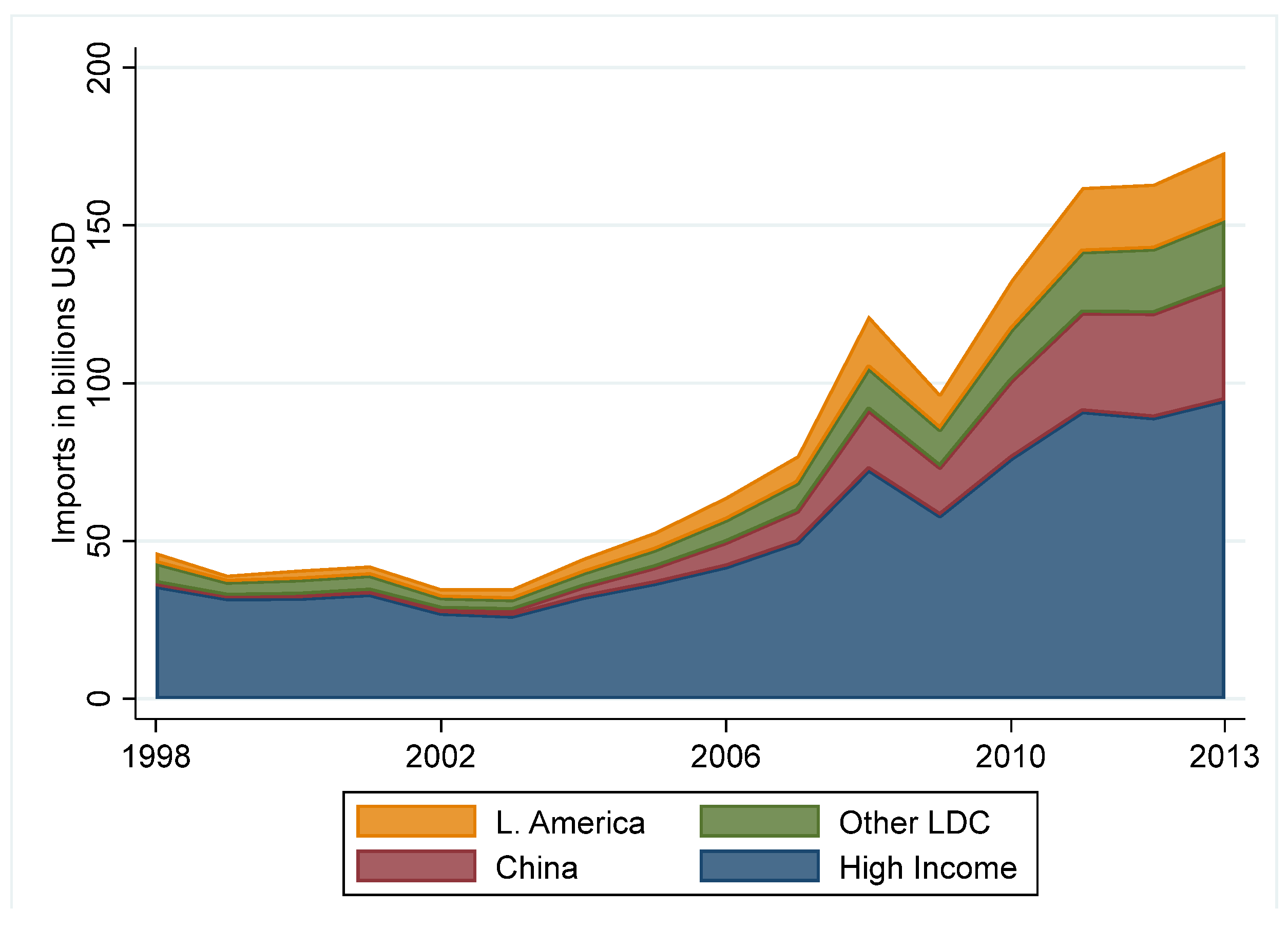
This subsection starts with an overview of the trade relationship between China and Brazil and of the import competition experienced by the Brazilian manufacturing sector. In 2000, Chinese imports made up 2.7 percent of Brazilian imports, which ranked it as the tenth largest exporter to Brazil. Yet, these figures were radically different in 2012, when Chinese imports amounted to approximately 20 percent of Brazilian imports, of which more than 90 percent are manufactured goods. Moreover, other labor abundant countries like India, Indonesia, and Vietnam accounted for less than one percent of Brazilian imports in this period (Paz 2019a). Figure 1 shows that imports from China and from high-income countries account for most Brazilian imports. Thus, ROW imports are mainly driven by imports from high income countries. Figure 1 also displays a growing Chinese share of Brazilian imports and a shrinkage of the high-income countries’ share. Indeed, both the Chinese and the ROW volume of imports grew over time, albeit at a different pace. Hence, the Brazilian experience in the 2000s cannot be summarized merely into a case of substitution of suppliers.
The import competition measure of Brazilian firms used in this study is the industry-level import penetration. This is the ratio between imports and the apparent consumption (production plus imports minus exports). In contrast with tariffs, the import penetration also captures the effects of NTMs, such as import licenses, quotas, and anti-dumping duties. Moreover, the import tariff between 2000 and 2012 shows little variability across industries and over time, despite the large variations in import volumes and in import penetration (Paz 2018). As a result, import tariffs are not recommended for the analysis carried out in this study.
Turning to the descriptive statistics at the industry level, Table 1 reports the 2000- and the 2012-level, the average, and the standard deviation of ROW and Chinese import penetrations. We can see that 19 out of 26 industries exhibited an increase in import penetration, and in most of these cases the increase was in excess of 20 percent. Most importantly, these industries employ more than half of the workers in manufacturing. Additionally, the Chinese import penetration grew in 24 out of 26 industries. Although the average Chinese import penetration is smaller than the ROW import penetration, the former has a significantly larger coefficient of variation due to the increase in Chinese participation in the Brazilian imports in this period. Together with Figure 1, these statistics indicate that this growth in Chinese import penetration was not simply a case of substitution of ROW imports. Table 1 also displays descriptive statistics for industry-level informality share. They show shares below 5 percent in industries such as automobiles, steel, and biofuels, while industries such as apparel and wood products exhibited an informality share close to 30 percent.
Table 2 presents industry-level average characteristics of manufacturing workers according to their formality status. The hourly wage consists of the monthly wage divided by 4.3 times the number of hours worked in a week. The inflation adjustment is conducted according to Corseuil and Foguel (2002) using inflating factors from IPEADATA (2017). The natural logarithm of the real hourly wage also exhibits heterogeneity across industries, being larger in skilled-labor intensive industries. These figures also indicate that formal workers earn substantially higher hourly wages and are more likely to be male. Formal workers are slightly older than informal workers. The industry-level average education level shows substantial cross-industry variation, which tend to be higher in skilled-labor-intensive industries such as pharmaceutical products. Even though formal workers are more educated on average, the difference in the average of years of schooling range from half year in footwear to three years in other chemical products. This study now turns to the presentation of the theoretical framework that motivates the description of the empirical methodology used here.
2.4. Theoretical Framework
The analysis of the effects of the changes in the trade openness of the Brazilian economy on the formal and informal labor market outcomes is guided by the theoretical model and empirical framework developed by Paz (2014)1. This is a heterogeneous firm model based on Melitz (2003), in which there is monopolistic competition and firms are heterogeneous in two dimensions: productivity and wages. Firms decide whether to enter the market or not considering their intrinsic characteristics and the current level of market competitiveness. If they decide to do so, what type of labor do firms offer to workers: formal or informal? By hiring formal workers, firms are subject to a fixed cost per worker to comply with labor regulations and a variable cost related to social security contributions. An informal labor contract has no such costs, but firms incur the risk of being audited (with positive probability) and fined if they are caught employing informal workers. In equilibrium, larger (more productive and higher wage) firms will hire only formal workers. In contrast, smaller (less productive and lower wage) firms will hire informal workers.
An increase in import penetration fosters competitiveness in domestic markets. This makes the smallest firms—who typically employ informal workers and pay lower wages—experience negative profits and exit the market. This leads to a reduction in the employment of informal workers and an increase in the average informal average wage. Yet the firms that were previously indifferent about hiring either formal or informal workers switch from formal to informal employment in response to this increased competitiveness. This raises the level of informal employment. Such a change may increase or decrease average formal and informal wages depending on the specific firm’s joint distribution of productivity and wages. In sum, an increase in import penetration leads to ex ante ambiguous effects of import penetration on informality and on average formal and informal wages.
An emerging literature has uncovered evidence of more nuanced effects of import competition depending on the source country of the imports and on the impacted industry characteristics. Facchini et al. (2010) found that the elasticity of substitution between Chinese and Brazilian manufacturing products was higher than that between Brazilian and high-income country products. This finding implies that imports from China are closer substitutes for Brazilian made goods. As a result, Chinese imports exert a stronger competitive pressure on Brazilian producers than imports from the rest of the world (especially those from high-income countries). This leads to the first testable prediction:
Hypothesis 1.
The effect of Chinese import penetration has a greater magnitude than that of ROW import penetration.
Moreira (2006) points out that China’s accession to the WTO exposed its trade partners to an unparalleled trade shock due to the uniqueness of the labor abundance of the Chinese economy relative to almost all countries in the world (Brazil included). Hence, according to the Heckscher-Ohlin model, unskilled-labor intensive imports from China apply a stronger competitive pressure than other imports. This is supported by Ashournia et al. (2014), who found that low-skill intensive firms in Denmark were heavily impacted by Chinese imports. Conversely, the competitiveness of ROW imports is milder in unskilled-labor intensive industries relative to that in other industries. This leads to the second testable prediction.
Hypothesis 2.
Increased Chinese import penetration has a larger effect on unskilled-labor intensive industries relative to its impact on other industries. Conversely, increased ROW import penetration affects other industries more than unskilled-labor intensive industries.
Another factor that can modulate the effects of import competition on labor market outcomes is the location of manufacturing activity. Indeed, this exhibits a significant spatial heterogeneity in Brazil, as 7 out of 26 states account for approximately 80 percent of all manufacturing activity (Paz 2019b). These seven states are those that make up the Southeastern and Southern regions of Brazil. According to Kapri and Paz (2019), such a spatial concentration makes manufacturing workers experience a different exposure to trade-induced shocks depending on their location. Thus, the effects of import penetration are expected to be different on workers in states with a large manufacturing sector. This leads to the third and last testable hypothesis:
Hypothesis 3.
Increased industry-level import penetration has a distinct impact on workers in manufacturing states relative to those in non-manufacturing states.
3. Empirical Methodology
The empirical methodology used to assess the testable hypotheses exploits the industry-level variation in competition induced by imports from China and from the ROW on the worker-level informality likelihood and on average formal and informal wages. Paz (2014) points out that decisions about the type of labor contract used (formal or informal) and the wage paid are made simultaneously. Hence, overlooking this simultaneity leads to biased estimates of the effects of import competition on wages. This was found to be the case in Brazil during the 1990s by Paz (2014) and in Peru during the 2000s by Pierola and Sanchez-Navarro (2019). Paz (2014) proposes addressing this simultaneity by means of the two-step switching regression framework from Maddala (1983). The first step in this framework is the regime selection equation that models the choice of the employment type using a Probit discrete choice specification, as depicted by Equation (1).
where is an indicator dependent variable that is “1” if worker i in industry j in state s and year t holds an informal job, and is “0” if worker holds a formal job; and is the respective latent variable. is the Chinese import penetration. is the ROW import penetration. is a vector of worker i’s observable characteristics, namely age, age squared, number of years of education, and indicators for gender, race, marital status, high school degree, and college degree. are industry fixed effects that control for the industry-specific and time-invariant characteristics. are state fixed effects which capture state specific and time-invariant characteristics, such as being landlocked. are year effects that account for time-varying factors that affect industries equally, such as business cycles. is the error term.
For identification purposes, the switching-regression framework requires the selection equation to contain at least one relevant variable that does not affect the wage earned by the worker. Following Paz (2014), the variable fulfilling this role is otherformalijst. This is a dummy variable that is “1” if another person in the household has a formal job, and “0” otherwise. The idea is that the tradeoff between a formal and an informal job experienced by a worker is affected by another household member having a formal job, since informal labor contracts are used by both firms and workers to evade taxation. In this vein, having another household with a formal job may increase the likelihood of detection of income tax evasion, and this reduces the incentives for choosing an informal job. This suggests a negative coefficient for this indicator variable in the selection equation.
The second step of the switching regression framework is to model the average wage through a Mincer-type wage () equation for each type of job using the inverse Mills ratio to control for the worker self-selection into that regime. The inverse Mills ratio (Λ(z)) is defined as Λ(z) ≡ ϕ(z)/Φ(z), where ϕ(z) is the standard normal distribution function and Φ(z) is the standard normal cumulative distribution function. It is calculated using the predicted values of the informality likelihood (). These wage equations are depicted by Equation (2) for the formal worker and by Equation (3) for the informal worker.
The selection into an informal or a formal labor contract takes place as a non-zero correlation among the error terms , , and . Should this be the case, the estimated coefficients of the inverse Mills ratios will be statistically significant. Accordingly, the omission of these terms will then lead to biased estimates of the effects of the import penetrations on wages. Note that the standard errors for Equations (2) and (3) are estimated by means of a 500-repetition bootstrap using household survey weights because the inverse Mills ratio is a generated regressor.
The calculation of the marginal effects of the import penetrations on wages ought to consider the effects of the import penetrations on the regime selection. This means that the effects of the import penetrations on wages will, in a non-trivial way, depend on the workers characteristics via the selection equation. The marginal effect of Chinese import penetration on the formal and the informal wages are given by Equations (4) and (5), respectively. The marginal effects for ROW import penetration are calculated in a similar fashion.
To assess the predictions of Hypothesis 2, Equations (1)–(3) are augmented to include new regressors that are interactions between the import penetration measures and , which is an indicator variable that is “1” for unskilled-labor intensive industries, and “0” otherwise. As in Paz and Ssozi (2021), the unskilled-labor intensive industries are the seven industries with the lowest average of year of schooling in 2000, namely food and beverages, textiles, apparel, footwear and leather products, wood products, non-metallic minerals and products, and furniture and other products. Similarly, Hypothesis 3 is evaluated through the addition to Equations (1)–(3) of interaction terms between the import penetrations and an indicator variable (Manufacturing states) that is “1” if state s is in the South or Southeast of Brazil, and “0” otherwise.
There are some concerns about the empirical methodology that deserve careful discussion. First, Brazilian producers may react slowly to changes in market conditions. This can be addressed by employing lagged import penetrations. The second concern is that both the import penetration measures and wages are simultaneously determined because the latter is part of the value added that is used in the calculation of the import penetration. This concern can also be alleviated by using the first lag of the import penetration measures.
The third concern is the omitted variable bias. More precisely, this could be the case of omitted time variant industry-specific shocks that affect both import penetrations and outcomes, and this biases the estimates. Examples of such omitted variables are demand or supply shocks in the Brazilian economy. For instance, suppose that a larger than expected import penetration increase leads the Brazilian government to impose higher import tariffs, safeguards, or countervailing duties. This behavior can be seen in the number of antidumping procedures initiated in Brazil that reached almost 100 cases in the 2000s, of which a quarter were against Chinese producers (cf. WTO Antidumping Gateway 2016). These product-level non-tariff protection measures cannot be accounted for in the empirical specification, and thus can bias the estimates. The use of an instrumental variable (IV) approach can address this concern, as explained next.
The excluded instruments used in the IV strategy are based upon Iacovone et al.’s (2013) idea of using supply-driven shocks as an instrument for import penetration.2 Thus, the excluded instrument for Chinese import penetration is the Chinese share of imports in third countries. The third countries considered have very small trade ties with Brazil and are located in Latin America, namely Mexico, Colombia, Costa Rica, Ecuador, El Salvador, Guatemala, Guyana, Jamaica, Nicaragua, Panama, and Peru. The correlation between the Chinese import penetration and Chinese share of imports in third countries is 0.574. The same endogeneity concern applies to the ROW import penetration; therefore, an additional excluded instrument is required. In a similar fashion, this is the high-income countries’ share in the imports of the above mentioned third countries. These high-income countries are Australia, Austria, Belgium, Bulgaria, Canada, Croatia, Czechia, Denmark, Finland, France, Germany, Greece, Hungary, Iceland, Ireland, Italy, Japan, Luxembourg, Netherlands, Norway, Poland, Portugal, Romania, Slovakia, Slovenia, Spain, Sweden, Switzerland, USA, and United Kingdom. The simple correlation between the ROW import penetration and the high-income share of imports is 0.316. In the specifications that include interaction terms between the import penetrations and indicator variables, the additional excluded instruments are built by interacting the excluded instruments mentioned above with the respective indicator variable.
Table 3 reports the estimated coefficients of the regressions of the endogenous explanatory variables (Chinese and ROW import penetrations) on the excluded instruments and other control variables used in the selection Equation (1). We can see that the Chinese share of imports in Latin America is statistically significant when the Chinese import penetration is the dependent variable, column (1), while the other excluded instrument is not significant. Similarly, the high-income countries’ share of imports in Latin America is significant in the specification for the ROW import penetration in column (2), whereas the Chinese share of imports in Latin America is not significant in this regression. None of the workers’ characteristics are statistically significant. These estimates show that the excluded instruments have predictive power over the endogenous regressors. The F-statistic of these regressions in Table 3 is above 200, which suggests that a weak instrument is not the problem.
4. Results and Discussion
This section begins with the estimates of the selection specification based on equation (1), which is the first step of the switching regression framework. Table 4 displays the estimated coefficients obtained using Probit in columns (1)–(3) and those obtained using IVProbit in columns (4)–(6). The worker’s characteristics’ estimated coefficients do not vary across specifications. They indicate that older, female, married, and Asian workers are more likely to hold an informal job, while black workers are less likely. The likelihood of having an informal job is smaller for those with a high school degree and with a larger number of years of schooling. Interestingly, the college degree indicator is not statistically significant at the 5 percent level in any specification. The other household member has a formal job indicator estimated coefficient which is negative and statistically significant in all specifications of Table 4, with a similar magnitude across specifications.
The Probit specifications do not display statistically significant coefficients for either the import penetrations or for their interactions. Additionally, notice that the null hypothesis of exogeneity of the endogenous regressors is rejected at the 5 percent level in all IVProbit specifications. This suggests that the focus of the analysis should be on the IV Probit specifications since they account for the endogeneity of the import penetrations and their interactions.
The IVProbit specification of column (4) displays no statistically significant coefficient of the Chinese and the ROW import penetration, therefore this result renders no support for Hypothesis 1. The specification in column (5) is designed to assess Hypothesis 2. It presents the Chinese and the ROW import penetrations with positive and statistically significant coefficients. The interaction terms of the import penetrations with the unskilled-labor intensive indicator are negative for both import penetrations, and statistically significant at the 5 percent level for the Chinese and at the 10 percent level for the ROW import penetration. These coefficients imply that an increase in any import penetration raises informality in non-unskilled-labor intensive industries. For unskilled-labor intensive industries, Chinese import penetration has no effect on informality, while ROW import penetration reduces informality in unskilled-labor intensive industries. These results do support that the Chinese and the ROW import penetrations have different impacts on informality (Hypothesis 1), and such impacts also depend on the unskilled-labor intensity of the industry. These results are not in line with Hypothesis 2. The estimates to assess Hypothesis 3 are in column (6), where both import penetrations are positive and significant as before. This means that increased import penetration leads to more informality in non-manufacturing states. The interaction terms with manufacturing state indicators are negative and significant. Accordingly, for manufacturing states Chinese import penetration reduces (albeit with a smaller magnitude) informality, whereas ROW import penetration has a positive effect. These results do support Hypothesis 3.
The results for ROW imports are somewhat distinct from those obtained by Paz (2014) using Brazilian data for the 1990s. His results indicate that greater imports—most from high income countries—increased the manufacturing informality share. On the one hand, Pierola and Sanchez-Navarro (2019) had IVProbit results of no effect regarding Chinese imports on informality for Peru in the 2000s, in line with this study findings. On the other hand, their findings that Chinese imports do increase informality among unskilled workers are at odds with the results of Table 4.
Table 5 reports the OLS and IV estimates employing equation (2) for the formal workers’ average wage in columns (1)–(3) and (4)–(6), respectively. The selection terms (the inverse Mills ratios) were computed using the IVProbit estimates of the specification that contained the same explanatory variables (except for the other formal indicator). The estimated coefficients of the selection terms are statistically significant in all columns. These coefficients are positive except in column (5). This is evidence that selection effects are taking place and should not be overlooked. The estimated coefficients for workers’ characteristics are stable across specifications. Formal workers’ wages are increasing with age and number of years of schooling, with considerable premium for high school and college degrees. Females and blacks earn a lower wage on average. Additionally, married and Asian workers have higher average wages. Notice that the OLS and the IV estimates for some variables are substantially different. In fact, the null of exogeneity of the import penetrations (and their interaction terms) is rejected at the 5 percent level in every column. Hence, the discussion will focus on the IV specifications results.
In column (4), the estimated coefficients of the Chinese import penetration are positive and statistically significant at the 5 percent level of confidence and the coefficient for the ROW import penetration is zero. As discussed in the previous section, the estimated coefficients of the import penetrations and their interactions are different from their marginal effects on the average wage due to the selection effect. The marginal effect is calculated for the average formal and informal worker, i.e., the estimated selection equation fitted at the average value of its regressors, as shown in Equation (4). The effects on the average formal wage of a percentage point increase in the Chinese import penetration is a 1.09 percent increase and for the ROW import penetration a 0.06 percent increase, respectively. These figures suggest that the Chinese and ROW import penetrations had a distinct impact on formal workers’ average wage, which supports Hypothesis 1.
The specification in column (5) shows that both the Chinese and the ROW import penetrations are positive and significant. The estimated coefficients of the interaction terms with the unskilled-labor intensive indicators were negative, though only the interaction with the ROW import penetration is significant. This means that the total effect of Chinese import penetration on the formal workers’ average wage for unskilled-labor intensive industries is positive, while the effect for the ROW import penetration in negative. For non-unskilled-labor intensive industries, the marginal effect on the average formal wage of a percentage point increase in the Chinese import penetration is a 3.47 percent increase, and for the ROW import penetration a 3.04 percent increase. For unskilled-labor intensive industries, these marginal effects are a 2.01 percent increase and a 4.28 percent decrease, respectively. These results are at odds with the predictions of Hypothesis 2. These results for average informal wages are at variance with the findings of Paz (2014) and Pierola and Sanchez-Navarro (2019). The former found a negative effect of ROW imports, and the latter found no effect of Chinese imports for the average worker, though their results for unskilled workers show a negative impact.
The estimates in column (6) display a positive coefficient for the Chinese import penetration and a negative for ROW import penetration. Both coefficients are statistically significant. The estimated coefficients of the interaction terms between the manufacturing state indicator and import penetrations are positive and significant. This means that, for manufacturing states, the total effects of both import penetrations are positive. For a formal worker located in a non-manufacturing state, the marginal effect on the average formal wage of a percentage point increase in the Chinese import penetration is a 0.1 percent decrease and for the ROW import penetration a 2.66 percent decrease. In manufacturing states, in contrast, these marginal effects are a 2.6 percent increase and a 0.64 percent increase, respectively. These estimates corroborate Hypothesis 3.
Table 6 reports the estimates for the average informal wage based on Equation (3). The OLS estimates are displayed in columns (1)–(3), and the IV estimates in columns (4)–(6). As in the previous table, the selection term estimated coefficients indicate the presence of selection effects. They are statistically significant in every specification, except in column (5). The estimated coefficients of the workers’ observable characteristics are stable across specifications. They present signs that are comparable to those in Table 5; however, the coefficients for female and years of schooling have a larger magnitude, while the coefficients for Asian, high school, and college indicators exhibit a smaller magnitude. As before, the null of exogeneity of the import penetrations is rejected at the 5 percent level in the IV specifications.
We can see in column (4) that the only statistically significant import penetration coefficient is for the ROW, which is positive. The marginal effect on the average informal wage of a percentage point increase in the Chinese import penetration is a 0.52 percent increase and for the ROW import penetration is a 3.39 percent increase. These figures support Hypothesis 1. The estimates in column (5) for both the Chinese and the ROW import penetrations are positive and significant at the 10 percent level. The coefficients of the interaction terms with the unskilled-labor intensive indicator are negative and not significant. Focusing on non-unskilled-labor intensive industries, the marginal effect on the average informal wage of a percentage point increase in the Chinese import penetration is a 5.4 percent increase and for the ROW import penetration a 5.3 percent increase. For the unskilled-labor intensive industries, these figures are a 0.12 percent increase and a 2.26 percent increase, respectively. These effects are at variance with the predictions of Hypothesis 2. These results for average formal wages are comparable to those of Paz (2014), who found a positive effect of ROW imports. Yet, Pierola and Sanchez-Navarro (2019) found no effect of Chinese imports on the average informal worker, and a negative effect for the unskilled informal worker.
The estimates in column (6) reveal that both import penetrations are negative, albeit not statistically significant. Their interactions with the manufacturing state indicator are positive, but only the interaction with the ROW import penetration is statistically significant. The marginal effect on the average informal wage of a percentage point increase in the Chinese import penetration is a 4.72 percent decrease, and for the ROW import penetration a 6.61 percent decrease for non-manufacturing states. The effects for manufacturing states are a 0.14 percent decline and a 2.23 percent increase, respectively. These different impacts on the average informal wage support Hypothesis 3.
Robustness Checks
The robustness check conducted here employs state-by-year fixed effects in lieu of state and year effects. This new specification is used to account for state specific policies such as changes in state-level educational systems, state-level minimum wages, and labor regulations enforcement (Almeida et al. 2022). Moreover, since commodity (iron ore or soybeans, for instance) production in Brazil is geographically concentrated in a few states, these state-by-year effects can also pick-up the effects of the increased Chinese demand for these primary commodities. Table 7 reports the Probit and IV Probit estimates of the selection equation using this new set of fixed effects. We can see that the results are very similar to those in Table 3. Table 8 reports the IV estimates for the average wage of informal workers in columns (1)–(3) and for the average wage of formal workers in columns (4)–(6). The estimates in columns (1)–(3) are very similar to those in columns (4)–(6) in Table 6. Moreover, these new estimates are more statistically significant in many cases. The specifications for the average wage of formal workers present estimated coefficients that are very similar in magnitude to those in columns (4)–(6) in Table 5. Nevertheless, their statistical significance has slightly declined. In sum, these estimates obtained using a different specification of fixed effects corroborates the results obtained with the main specifications.
5. Conclusions
China is one of the most populous countries in the world, and it entered the 21st century not only as one of the largest and fast-growing economies but also as a major player in world trade. This rather swift ascension together with its cost advantage in manufacturing production prompted several concerns in developing countries as to whether they would still be able to sustain a dynamic manufacturing sector in view of this Chinese competitive edge. Such concern is built on the fact that many observers perceive a strong manufacturing sector as a key driver of economic growth and as a provider of higher wage jobs relative to those available in agriculture and services.
A good case study to assess such concerns is the increase in import competition experienced by the Brazilian manufacturing sector in 2000–2012. In this period, the import penetration increased by more than 20 percent and the Chinese share of such imports increased from 3 to 20 percent. Brazil is also the largest economy of Latin America and has a large and diverse manufacturing sector with ubiquitous informal employment.
This study employed Brazilian household data to examine the impacts of the increasing Chinese and rest of the world import penetrations on the likelihood of informal employment and on the average wage of formal and informal workers in the manufacturing sector for 2000–2012. The empirical methodology employs a switching regressions model as in Paz (2014), which accounts for worker self-selection into formal and informal jobs and for the potential endogeneity of trade policy.
The empirical results indicate that greater industry-level Chinese and ROW import penetrations increase the informal job likelihood at different intensities. Furthermore, these effects are heterogeneous and modulated by the unskilled labor intensity of the industry and by the degree of industrialization of the Brazilian states. Indeed, the ROW import penetration has a negative effect, and the Chinese import penetration has no effect on the informality likelihood in unskilled-labor intensive industries. In contrast, both import penetrations have positive impact on informality likelihood in the remaining industries. An increase in the Chinese import penetration reduces informality while ROW import penetration increases it in manufacturing states. Nevertheless, both forms of import penetration positively affect informality in non-manufacturing states.
The effects on the average formal and informal wages are more nuanced. An increase in Chinese import penetration raises the average formal wage, except in manufacturing states. Greater ROW import penetration decreases the average formal wage, except for in manufacturing states or in non-unskilled-labor intensive industries. For the average informal wage, both the Chinese and the ROW import penetration have positive effects of different magnitudes, and negative effects for informal workers located in non-manufacturing states.
The evidence amassed in this study suggests that the effects of international trade on labor market outcomes are moderated by the country of origin of imports and, at the same time, by the unskilled labor intensity of industries and by regional characteristics. The important nuances uncovered by this study should not be overlooked in the design of public policies to address potential harmful effects of increased import competition, especially because the most vulnerable workers seem to experience a negative impact from this trade.
Moreover, this study’s estimates are at variance with those of the extant literature for different countries and periods of time. This strongly suggests that such trade effects are highly heterogeneous. Unfortunately, data scarcity that plagues the entire literature—such as the lack of employee–employer matched data covering informal jobs—is a major limitation of this study because it precludes an investigation of the role of either the unobservable characteristics of workers or firm characteristics. Given the available data, a promising avenue for future research is the use of cross-country data to investigate whether country-specific institutions are behind these disparate results.
Funding
This research received no external funding.
Data Availability Statement
The data used in this article can be found at www.ibge.gov.br and ipeadata.gov.br.
Conflicts of Interest
The author declares no conflict of interest.
| 1. | This type of ambiguity is also present in other models of informal labor like Goldberg and Pavcnik (2003) and Aleman-Castilla (2006). |
| 2. |
References
- Aleman-Castilla, Benjamin. 2006. The Effect of Trade Liberalization on Informality and Wages: Evidence from Mexico. CEP Discussion Paper No. 763. London: Centre for Economic Performance, London School of Economics and Political Science. [Google Scholar]
- Aleman-Castilla, Benjamin. 2020. Trade and Labour Market Outcomes Theory and Evidence at the Firm and Worker Levels. ILO Working Paper 12. Geneva: ILO. [Google Scholar]
- Almeida, Rita, Lourenço S. Paz, and Jennifer P. Poole. 2022. Precarization or Protection? The Impact of Trade and Labour Policies on Informality. Helsinki: The United Nations University World Institute for Development Economics Research (UNU-WIDER). [Google Scholar]
- Araújo, Bruno César, and Lourenço S. Paz. 2014. The Effects of Exporting on Wages: An Evaluation Using the 1999 Brazilian Exchange Rate Devaluation. Journal of Development Economics 111: 1–16. [Google Scholar] [CrossRef]
- Ashournia, Damoun, Jakob Roland Munch, and Daniel Nguyen. 2014. The Impact of Chinese Import Penetration on Danish Firms and Workers. IZA Discussion Paper No. 8166. Bonn: Institute for the Study of Labor. [Google Scholar]
- Baumann, Renato. 2001. Brazil in the 1990s: An economy in transition. CEPAL Review 73: 147–69. [Google Scholar] [CrossRef]
- Chandra, Piyush. 2014. WTO subsidy rules and tariff liberalization: Evidence from accession of China. The Journal of International Trade & Economic Development 23: 1170–205. [Google Scholar]
- Corseuil, Carlos Henrique, and Miguel Nathan Foguel. 2002. Uma Sugestão de Deflatores Para Rendas Obtidas a Partir de Algumas Pesquisas Domiciliares do IBGE. Textos Para Discussão, IPEA TD 0897. Brasília: Ipea. [Google Scholar]
- Dávalos, Jorge. 2019. Trade openness effects on informality and the real exchange rate channel. Applied Economics Letters 26: 506–10. [Google Scholar] [CrossRef]
- Facchini, Giovanni, Marcelo Olarreaga, Peri Silva, and Gerald Willmann. 2010. Substitutability and Protectionism: Latin America’s Trade Policy and Imports from China and India. The World Bank Economic Review 24: 446–73. [Google Scholar] [CrossRef] [Green Version]
- Goldberg, Pinelopi Koujianou, and Nina Pavcnik. 2003. The response of the informal sector to trade liberalization. Journal of Development Economics 72: 463–96. [Google Scholar] [CrossRef] [Green Version]
- Iacovone, Leonardo, Ferdinand Rauch, and L. Alan Winters. 2013. Trade as an engine of creative destruction: Mexican experience with Chinese competition. Journal of International Economics 89: 379–92. [Google Scholar] [CrossRef] [Green Version]
- IBGE. 2015. Banco de Dados Agregados. Sistema IBGE de Recuperação Automática—SIDRA. Available online: https://sidra.ibge.gov.br/home/pimpfbr/brasil (accessed on 11 April 2021).
- IBGE. 2016. Tabelas Sinóticas Retropoladas 2000–2013. Available online: https://www.ibge.gov.br/estatisticas/economicas/comercio/9052-sistema-de-contas-nacionais-brasil.html (accessed on 12 April 2021).
- IPEADATA. 2017. Instituto de Pesquisa Economica Aplicada. Available online: http://ipeadata.gov.br (accessed on 11 April 2021).
- Kapri, Kul Prasad, and Lourenço S. Paz. 2019. The Effects of the Chinese imports on Brazilian Manufacturing Workers. Economies 7: 76. [Google Scholar]
- Kume, Honório, Guida Piani, and Carlos Souza. 2003. Instrumentos de Política Comercial no Periodo 1987–1998. In A Abertura Comercial Brasileira nos anos 1990: Impactos Sobre Emprego e Salário. Edited by Carlos Henrique Corseuil and Honório Kume. Rio de Janeiro, Brazil: Ipea. [Google Scholar]
- Kume, Honorio, Guida Piani, and Pedro Miranda. 2008. Política Comercial, Instituições e Crescimento Economico no Brasil. In Crecimiento Económico, Instituciones, Política Comercial y Defensa de la Competencia en el Mercosur. Edited by Honorio Kume. Montevidéu: Red Mercosur, vol. 11. [Google Scholar]
- Maddala, Gangadharrao S. 1983. Limited-Dependent and Qualitative Variables in Economics. Cambridge: Cambridge University Press. [Google Scholar]
- Melitz, Marc J. 2003. The Impact of Trade on Intra-Industry Reallocations and Aggregate Industry Productivity. Econometrica 71: 1695–725. [Google Scholar] [CrossRef] [Green Version]
- Moreira, Mauricio Mesquita. 2006. Fear of China: Is There a Future for Manufacturing in Latin America? Intal-ITD, Occasional paper 36. Buenos Aires: Intal. [Google Scholar]
- Paz, Lourenço S. 2014. The Impacts of Trade Liberalization on Informal Labor Markets: A Theoretical and Empirical Evaluation of the Brazilian Case. Journal of International Economics 92: 330–48. [Google Scholar] [CrossRef] [Green Version]
- Paz, Lourenço S. 2018. The effect of import competition on Brazil’s Manufacturing Labor Market in the 2000s: Are imports from China different? The International Trade Journal 32: 76–99. [Google Scholar] [CrossRef]
- Paz, Lourenço S. 2019a. Chinese imports’ impacts on Brazil’s Inter-Industry Wage Premium. Journal of Economic Studies 46: 1052–64. [Google Scholar] [CrossRef]
- Paz, Lourenço S. 2019b. The Impact of the China Shock on the Manufacturing Labor Market in Brazil. IDB WORKING PAPER SERIES N° IDB-WP-01085. Washington, DC: Inter-American Development Bank. [Google Scholar]
- Paz, Lourenço S. 2021. How does import competition impact job type? Economics Bulletin 41: 2063–20. [Google Scholar]
- Paz, Lourenço S., and John Ssozi. 2021. The Effects of Chinese Imports on Female Workers in the Brazilian Manufacturing Sector. The Journal of Development Studies 57: 807–23. [Google Scholar] [CrossRef]
- Pierola, Martha Denisse, and Dennis Sanchez-Navarro. 2019. Import Competition in the Manufacturing Sector in Peru: Its Impact on Informality and Wages. IDB WORKING PAPER SERIES N° IDB-WP-01093. Washington, DC: Inter-American Development Bank. [Google Scholar]
- United Nations. 2003. Statistical Division. UN Comtrade. New York: United Nations. [Google Scholar]
- WTO Antidumping Gateway. 2016. World Trade Organization, Geneva, Switzerland. Available online: https://www.wto.org/english/tratop_e/adp_e/adp_e.htm (accessed on 10 April 2021).
Figure 1.
Brazilian manufacturing imports by source. Notes: L. America–Latin America. Other LDC–developing countries other than China and those in Latin America.
Figure 1.
Brazilian manufacturing imports by source. Notes: L. America–Latin America. Other LDC–developing countries other than China and those in Latin America.


Table 1.
Industry-level trade exposure and labor market characteristics of manufacturing industries in Brazil during 2000–2012.
Table 1.
Industry-level trade exposure and labor market characteristics of manufacturing industries in Brazil during 2000–2012.
| Industry/Year | ROW Import Penetration (%) | Chinese Import Penetration (%) | Informal Share (%) | |||||||||
|---|---|---|---|---|---|---|---|---|---|---|---|---|
| 2000 | 2012 | Mean | S. dv. | 2000 | 2012 | Mean | S. dv. | 2000 | 2012 | Mean | S. dv. | |
| Food and Beverages | 4.33 | 3.53 | 3.87 | 0.42 | 0.05 | 0.65 | 0.21 | 0.17 | 20.40 | 21.05 | 19.45 | 39.58 |
| Tobacco | 27.61 | 27.38 | 26.90 | 1.49 | 0.22 | 2.19 | 1.48 | 1.15 | 6.96 | 11.51 | 10.69 | 30.91 |
| Textiles | 9.45 | 9.20 | 8.88 | 0.81 | 0.23 | 6.44 | 2.38 | 2.26 | 17.78 | 46.67 | 25.16 | 43.39 |
| Apparel | 2.90 | 6.31 | 3.98 | 1.00 | 0.17 | 5.45 | 2.20 | 1.78 | 22.28 | 53.31 | 29.26 | 45.50 |
| Footwear and leather products | 5.67 | 5.67 | 5.08 | 0.48 | 0.56 | 2.66 | 1.49 | 0.78 | 20.16 | 19.59 | 17.12 | 37.67 |
| Wood products | 2.54 | 1.34 | 2.00 | 0.63 | 0.07 | 0.47 | 0.18 | 0.12 | 25.00 | 51.95 | 28.20 | 45.00 |
| Paper products | 10.59 | 7.45 | 8.97 | 1.58 | 0.01 | 0.85 | 0.21 | 0.23 | 11.25 | 10.34 | 9.51 | 29.33 |
| Printing and Publishing | 0.62 | 1.50 | 0.97 | 1.01 | 0.00 | 0.15 | 0.04 | 0.05 | 25.81 | 24.86 | 25.64 | 43.66 |
| Petroleum refining | 0.00 | 4.33 | 9.65 | 1.84 | 0.00 | 0.00 | 0.18 | 0.12 | 6.79 | 12.86 | 7.21 | 25.87 |
| Biofuel | 20.64 | 26.63 | 0.59 | 1.09 | 0.43 | 1.65 | 0.00 | 0.00 | 7.36 | 1.17 | 3.31 | 17.89 |
| Pharmaceutical products | 19.62 | 26.01 | 23.17 | 2.66 | 0.00 | 0.97 | 0.93 | 0.47 | 8.90 | 6.08 | 8.05 | 27.21 |
| Cleaning products | 7.02 | 6.60 | 20.98 | 1.84 | 0.01 | 0.21 | 0.28 | 0.29 | 15.63 | 8.63 | 15.41 | 36.11 |
| Paint and varnish | 9.56 | 10.79 | 6.10 | 1.04 | 0.14 | 2.55 | 0.06 | 0.05 | 9.13 | 5.83 | 9.00 | 28.63 |
| Rubber and plastic products | 6.83 | 9.64 | 9.77 | 0.43 | 0.10 | 2.88 | 0.88 | 0.78 | 11.52 | 12.75 | 9.91 | 29.88 |
| Steel | 22.54 | 24.80 | 8.07 | 1.61 | 0.27 | 1.58 | 1.59 | 1.45 | 6.18 | 5.47 | 4.83 | 21.43 |
| Non-ferrous metals | 7.61 | 8.20 | 22.78 | 1.97 | 0.30 | 3.05 | 0.73 | 0.48 | 12.28 | 5.78 | 10.29 | 30.39 |
| Metal products | 26.11 | 21.63 | 7.42 | 0.28 | 0.26 | 4.63 | 1.25 | 0.84 | 17.42 | 31.57 | 16.95 | 37.52 |
| Machinery and equipment | 1.36 | 0.91 | 22.68 | 3.14 | 0.24 | 2.43 | 1.97 | 1.66 | 13.76 | 12.42 | 12.60 | 33.18 |
| Appliances | 24.71 | 22.11 | 0.99 | 0.32 | 0.02 | 1.30 | 0.99 | 0.77 | 6.57 | 5.06 | 6.06 | 23.87 |
| Auto Parts | 55.64 | 32.86 | 21.02 | 3.97 | 0.26 | 3.61 | 0.34 | 0.34 | 11.01 | 6.53 | 8.49 | 27.88 |
| Other transp. Equipment | 4.90 | 4.60 | 39.86 | 12.09 | 0.12 | 2.38 | 0.96 | 0.71 | 21.33 | 14.60 | 14.78 | 35.49 |
| Non-metallic min. and products | 45.08 | 32.43 | 4.47 | 0.56 | 2.07 | 18.22 | 0.87 | 0.77 | 30.31 | 24.00 | 29.79 | 45.73 |
| Office, electrical, electronic, optical, precision, and communication equipment | 13.73 | 15.37 | 39.94 | 5.83 | 0.00 | 0.39 | 8.36 | 6.72 | 13.97 | 13.89 | 12.95 | 33.58 |
| Automobiles, trucks, and buses | 26.69 | 30.16 | 12.93 | 1.55 | 0.59 | 3.45 | 0.18 | 0.19 | 5.20 | 3.60 | 4.18 | 20.02 |
| Other chemical products | 4.84 | 4.03 | 26.75 | 1.38 | 1.27 | 5.31 | 1.45 | 0.96 | 13.44 | 11.02 | 14.91 | 35.62 |
| Furniture and other products | 4.33 | 3.53 | 4.04 | 0.58 | 0.05 | 0.65 | 3.28 | 1.54 | 28.04 | 44.86 | 24.41 | 42.96 |
Notes: Informal workers are those without social security coverage. Number of observations is 312. Household survey weights used for informal share.
Table 2.
Formal and Informal workers’ average characteristics at industry level.
| Industry/Year | Log (Hourly Wage) | Age | Female Share (%) | Years of Schooling | ||||
|---|---|---|---|---|---|---|---|---|
| Formal | Informal | Formal | Informal | Formal | Informal | Formal | Informal | |
| Food and Beverages | 1.468 | 0.917 | 33.085 | 32.326 | 0.266 | 0.370 | 7.062 | 5.737 |
| Tobacco | 1.611 | 0.933 | 36.011 | 33.143 | 0.393 | 0.525 | 7.638 | 6.226 |
| Textiles | 1.338 | 0.573 | 33.154 | 33.985 | 0.499 | 0.717 | 7.309 | 6.139 |
| Apparel | 1.289 | 1.017 | 36.285 | 35.975 | 0.837 | 0.843 | 7.094 | 6.840 |
| Footwear and leather products | 1.332 | 1.076 | 30.934 | 30.661 | 0.477 | 0.514 | 7.260 | 6.766 |
| Wood products | 1.340 | 1.042 | 34.910 | 31.956 | 0.168 | 0.129 | 5.687 | 5.077 |
| Paper products | 1.796 | 1.312 | 32.940 | 30.561 | 0.201 | 0.317 | 8.548 | 7.594 |
| Printing and Publishing | 1.866 | 1.467 | 32.534 | 30.062 | 0.277 | 0.297 | 9.361 | 8.914 |
| Petroleum refining | 2.446 | 2.204 | 36.709 | 35.769 | 0.134 | 0.193 | 10.287 | 10.262 |
| Biofuel | 1.625 | 1.270 | 33.767 | 33.830 | 0.109 | 0.085 | 6.776 | 5.702 |
| Pharmaceutical products | 2.131 | 1.743 | 32.530 | 31.317 | 0.437 | 0.437 | 10.864 | 10.066 |
| Cleaning products | 1.750 | 1.375 | 32.278 | 31.475 | 0.409 | 0.475 | 9.129 | 8.016 |
| Paint, varnish, and laqueur | 1.957 | 1.591 | 32.758 | 31.393 | 0.178 | 0.202 | 9.203 | 8.645 |
| Rubber and plastic products | 1.722 | 1.346 | 32.162 | 30.531 | 0.249 | 0.292 | 8.302 | 7.498 |
| Steel | 2.080 | 1.616 | 34.845 | 32.308 | 0.079 | 0.162 | 9.202 | 8.198 |
| Non-ferrous metals | 1.892 | 1.368 | 33.914 | 31.185 | 0.124 | 0.147 | 8.856 | 7.558 |
| Metal products | 1.816 | 1.302 | 34.089 | 31.526 | 0.105 | 0.085 | 7.799 | 6.902 |
| Machinery and equipment | 1.920 | 1.544 | 34.092 | 32.706 | 0.108 | 0.127 | 8.668 | 7.687 |
| Appliances | 1.832 | 1.396 | 31.336 | 29.532 | 0.276 | 0.276 | 9.642 | 8.454 |
| Auto Parts | 1.895 | 1.463 | 32.339 | 30.278 | 0.170 | 0.177 | 8.938 | 7.919 |
| Other transportation equipment | 1.995 | 1.496 | 34.004 | 33.641 | 0.111 | 0.108 | 9.038 | 7.167 |
| Non-metallic minerals and products | 1.476 | 0.941 | 33.044 | 29.233 | 0.112 | 0.102 | 6.454 | 5.105 |
| Office, electrical, electronic, optical, precision, and communication equipment | 1.860 | 1.538 | 31.589 | 30.646 | 0.315 | 0.255 | 9.629 | 8.894 |
| Automobiles, trucks, and buses | 2.298 | 1.773 | 33.389 | 30.367 | 0.128 | 0.225 | 10.015 | 8.932 |
| Other chemical products | 1.991 | 1.064 | 34.097 | 32.576 | 0.207 | 0.217 | 9.285 | 5.809 |
| Furniture and other products | 1.601 | 1.087 | 33.541 | 31.521 | 0.258 | 0.239 | 7.615 | 6.811 |
Notes: Number of observations is 669,966. Informal workers are those without social security coverage. Household survey weights used.
Table 3.
First-stage OLS regressions of the endogenous regressors.
| Regressors/Dependent Variable | (1) | (2) | (3) | (4) |
|---|---|---|---|---|
| Chinese Import Penetrationt−1 | ROW Import Penetrationt−1 | Chinese Import Penetrationt−1 | ROW Import Penetrationt−1 | |
| Chinese share of imports in LAt−1 | 9.831 ** | −8.861 | 9.780 ** | −8.794 |
| (4.452) | (6.576) | (4.356) | (6.376) | |
| High Income countries share of imports in LAt−1 | −4.108 | −10.112 ** | −4.238 | −9.743 ** |
| (2.466) | (5.027) | (2.523) | (4.495) | |
| Age | −0.001 | 0.006 * | −0.001 | 0.005 |
| (0.002) | (0.003) | (0.002) | (0.003) | |
| Age2 | 0.000 | −0.000 * | 0.000 | −0.000 |
| (0.000) | (0.000) | (0.000) | (0.000) | |
| Female | −0.009 | −0.008 | −0.010 | −0.003 |
| (0.011) | (0.014) | (0.009) | (0.011) | |
| Married | −0.005 | −0.056 * | −0.005 | −0.055 * |
| (0.019) | (0.032) | (0.018) | (0.031) | |
| Black | 0.000 | 0.009 | 0.004 | 0.002 |
| (0.005) | (0.013) | (0.008) | (0.014) | |
| Asian | −0.008 | −0.013 | −0.012 | 0.005 |
| (0.018) | (0.086) | (0.015) | (0.074) | |
| Years of schooling | −0.003 | 0.007 | −0.002 | 0.004 |
| (0.003) | (0.006) | (0.002) | (0.004) | |
| High school | 0.004 | −0.023 | −0.001 | −0.005 |
| (0.005) | (0.019) | (0.006) | (0.015) | |
| College | 0.020 | −0.040 | 0.017 | −0.033 |
| (0.019) | (0.040) | (0.016) | (0.035) | |
| Other household has a formal jobijst | 0.009 | −0.008 | 0.007 | −0.004 |
| (0.007) | (0.011) | (0.007) | (0.010) | |
| Industry, state, and year fixed effects | Yes | Yes | No | No |
| Industry and state-year fixed effects | No | No | Yes | Yes |
| F-statistic | 392.14 | 570.5 | 201.36 | 335.88 |
Number of observations is 671,134. **, and * indicate statistical significance at the 5%, and 10% levels, respectively. Standard errors clustered at industry level are reported in parenthesis. Household survey weights used.
Table 4.
Worker-level Probit (1–3) and IVProbit (4–6) estimates of the effects of industry-level import penetration on the informal status indicator, using Equation (1).
Table 4.
Worker-level Probit (1–3) and IVProbit (4–6) estimates of the effects of industry-level import penetration on the informal status indicator, using Equation (1).
| Regressors | (1) | (2) | (3) | (4) | (5) | (6) |
|---|---|---|---|---|---|---|
| Chinese import penetrationt−1 | −0.010 | −0.003 | 0.000 | 0.002 | 0.085 ** | 0.031 *** |
| (0.014) | (0.010) | (0.015) | (0.007) | (0.034) | (0.008) | |
| ROW import penetrationt−1 | −0.006 | −0.002 | −0.007 | 0.017 | 0.069 *** | 0.045 *** |
| (0.005) | (0.004) | (0.005) | (0.013) | (0.026) | (0.014) | |
| Chinese imp. penet.t−1 × L. int.j | −0.015 | −0.083 *** | ||||
| (0.017) | (0.030) | |||||
| ROW imp. penet.t−1 × L. int.j | −0.004 | −0.113 * | ||||
| (0.024) | (0.065) | |||||
| Chinese imp. penet.t−1 × Manuf.s | −0.014 | −0.039 *** | ||||
| (0.010) | (0.006) | |||||
| ROW imp. penet.t−1 × Manuf.s | 0.001 | −0.035 *** | ||||
| (0.004) | (0.003) | |||||
| Age | −0.120 *** | −0.120 *** | −0.120 *** | −0.120 *** | −0.119 *** | −0.119 *** |
| (0.008) | (0.008) | (0.008) | (0.002) | (0.002) | (0.002) | |
| Age2 | 0.002 *** | 0.002 *** | 0.002 *** | 0.002 *** | 0.002 *** | 0.002 *** |
| (0.000) | (0.000) | (0.000) | (0.000) | (0.000) | (0.000) | |
| Female | 0.463 *** | 0.463 *** | 0.463 *** | 0.463 *** | 0.459 *** | 0.456 *** |
| (0.091) | (0.091) | (0.091) | (0.008) | (0.008) | (0.008) | |
| Married | 0.133 *** | 0.132 *** | 0.133 *** | 0.135 *** | 0.131 *** | 0.135 *** |
| (0.035) | (0.036) | (0.035) | (0.008) | (0.008) | (0.008) | |
| Black | −0.079 *** | −0.079 *** | −0.079 *** | −0.079 *** | −0.079 *** | −0.080 *** |
| (0.023) | (0.023) | (0.023) | (0.013) | (0.013) | (0.013) | |
| Asian | 0.196 *** | 0.196 *** | 0.197 *** | 0.197 *** | 0.196 *** | 0.211 *** |
| (0.049) | (0.049) | (0.049) | (0.054) | (0.053) | (0.054) | |
| Years of schooling | −0.028 *** | −0.028 *** | −0.028 *** | −0.028 *** | −0.028 *** | −0.028 *** |
| (0.006) | (0.006) | (0.006) | (0.001) | (0.001) | (0.001) | |
| High school | −0.176 *** | −0.175 *** | −0.175 *** | −0.175 *** | −0.173 *** | −0.172 *** |
| (0.018) | (0.018) | (0.018) | (0.011) | (0.011) | (0.011) | |
| College | 0.018 | 0.017 | 0.019 | 0.018 | 0.018 | 0.036 * |
| (0.033) | (0.033) | (0.034) | (0.020) | (0.020) | (0.020) | |
| Other household has a formal jobijst | −0.345 *** | −0.345 *** | −0.345 *** | −0.345 *** | −0.343 *** | −0.344 *** |
| (0.020) | (0.020) | (0.020) | (0.007) | (0.007) | (0.007) | |
| Exogeneity test | 7.724 ** | 36.47 *** | 126.6 *** | |||
| (0.021) | (0.000) | (0.000) |
Notes: Number of observations is 671,134. ***, **, and * indicate statistical significance at the 1%, 5%, and 10% levels, respectively. Standard errors clustered at the industry level. Sample weights from PNAD/Census used. State, industry, and year fixed effects included in the estimated model. The excluded instruments are the Latin American countries’ Chinese share of imports, the Latin American countries’ high-income countries share of imports, and their interactions.
Table 5.
Worker-level IV estimates of the effects of industry-level import penetration on the wages of formal workers using Equation (2).
Table 5.
Worker-level IV estimates of the effects of industry-level import penetration on the wages of formal workers using Equation (2).
| Regressors | (1) | (2) | (3) | (4) | (5) | (6) |
|---|---|---|---|---|---|---|
| Chinese import penetrationt−1 | −0.003 ** | −0.009 *** | 0.002 | 0.011 *** | 0.028 ** | 0.009 *** |
| (0.002) | (0.002) | (0.002) | (0.003) | (0.012) | (0.003) | |
| ROW import penetrationt−1 | 0.001 | −0.003 ** | −0.002 ** | −0.000 | 0.025 ** | −0.012 ** |
| (0.001) | (0.001) | (0.001) | (0.005) | (0.012) | (0.005) | |
| Chinese imp. penet.t−1 × L. int.j | 0.028 *** | −0.008 | ||||
| (0.003) | (0.020) | |||||
| ROW imp. penet.t−1 × L. int.j | −0.013 *** | −0.066 ** | ||||
| (0.003) | (0.028) | |||||
| Chinese imp. penet.t−1 × Manuf.s | −0.006 *** | 0.015 *** | ||||
| (0.001) | (0.004) | |||||
| ROW imp. penet.t−1 × Manuf.s | 0.004 *** | 0.021 *** | ||||
| (0.000) | (0.002) | |||||
| Age | 0.053 *** | 0.055 *** | 0.053 *** | 0.055 *** | 0.043 *** | 0.015 *** |
| (0.001) | (0.001) | (0.001) | (0.001) | (0.001) | (0.004) | |
| Age2 | −0.000 *** | −0.001 *** | −0.000 *** | −0.001 *** | −0.000 *** | 0.021 *** |
| (0.000) | (0.000) | (0.000) | (0.000) | (0.000) | (0.002) | |
| Female | −0.285 *** | −0.292 *** | −0.282 *** | −0.290 *** | −0.247 *** | 0.078 *** |
| (0.003) | (0.003) | (0.003) | (0.003) | (0.006) | (0.002) | |
| Married | 0.028 *** | 0.027 *** | 0.028 *** | 0.027 *** | 0.035 *** | −0.001 *** |
| (0.002) | (0.002) | (0.002) | (0.002) | (0.002) | (0.000) | |
| Black | −0.080 *** | −0.078 *** | −0.081 *** | −0.079 *** | −0.088 *** | −0.375 *** |
| (0.004) | (0.004) | (0.004) | (0.004) | (0.004) | (0.008) | |
| Asian | 0.151 *** | 0.148 *** | 0.151 *** | 0.151 *** | 0.166 *** | 0.011 *** |
| (0.015) | (0.015) | (0.015) | (0.015) | (0.015) | (0.003) | |
| Years of schooling | 0.047 *** | 0.047 *** | 0.047 *** | 0.047 *** | 0.044 *** | −0.061 *** |
| (0.000) | (0.000) | (0.000) | (0.000) | (0.000) | (0.004) | |
| High school | 0.107 *** | 0.109 *** | 0.106 *** | 0.108 *** | 0.093 *** | 0.110 *** |
| (0.004) | (0.004) | (0.004) | (0.004) | (0.005) | (0.015) | |
| College | 0.700 *** | 0.699 *** | 0.700 *** | 0.699 *** | 0.707 *** | 0.054 *** |
| (0.009) | (0.009) | (0.009) | (0.009) | (0.009) | (0.001) | |
| Inverse Mills ratio | 0.080 *** | 0.118 *** | 0.065 *** | 0.104 *** | −0.124 *** | 0.573 *** |
| (0.013) | (0.013) | (0.013) | (0.014) | (0.033) | (0.050) | |
| Endogeneity test | 39.24 *** | 22.32 *** | 115.62 *** | |||
| (0.000) | (0.000) | (0.000) | ||||
| Technique | OLS | OLS | OLS | IV | IV | IV |
Notes: Number of observations is 533,584. *** and ** indicate statistical significance at the 1% and 5% levels, respectively. Standard errors are bootstrapped with 500 repetitions. Sample weights from PNAD/Census used. State, industry, and year fixed effects included in the estimated model.
Table 6.
Worker-level IV estimates of the effects of industry-level import penetration on the wages of informal workers using Equation (3).
Table 6.
Worker-level IV estimates of the effects of industry-level import penetration on the wages of informal workers using Equation (3).
| Regressors | (1) | (2) | (3) | (4) | (5) | (6) |
|---|---|---|---|---|---|---|
| Chinese import penetrationt−1 | 0.012 *** | −0.002 | 0.015 *** | 0.005 | 0.046 * | −0.019 |
| (0.004) | (0.006) | (0.005) | (0.008) | (0.025) | (0.019) | |
| ROW import penetrationt−1 | 0.010 *** | −0.001 | −0.001 | 0.032 *** | 0.046 * | −0.025 |
| (0.002) | (0.004) | (0.003) | (0.009) | (0.025) | (0.018) | |
| Chinese imp. penet.t−1 × L. int.j | 0.021 *** | −0.045 | ||||
| (0.007) | (0.028) | |||||
| ROW imp. penet.t−1 × L. int.j | 0.006 | −0.018 | ||||
| (0.007) | (0.030) | |||||
| Chinese imp. penet.t−1 × Manuf.s | −0.007 ** | 0.010 | ||||
| (0.003) | (0.014) | |||||
| ROW imp. penet.t−1 × Manuf.s | 0.009 *** | 0.058 *** | ||||
| (0.001) | (0.014) | |||||
| Age | 0.054 *** | 0.067 *** | 0.070 *** | 0.051 *** | 0.052 *** | 0.138 *** |
| (0.002) | (0.003) | (0.003) | (0.002) | (0.006) | (0.020) | |
| Age2 | −0.001 *** | −0.001 *** | −0.001 *** | −0.000 *** | −0.000 *** | −0.002 *** |
| (0.000) | (0.000) | (0.000) | (0.000) | (0.000) | (0.000) | |
| Female | −0.374 *** | −0.436 *** | −0.450 *** | −0.363 *** | −0.363 *** | −0.766 *** |
| (0.010) | (0.012) | (0.013) | (0.011) | (0.030) | (0.093) | |
| Married | 0.026 *** | 0.015 ** | 0.013 ** | 0.029 *** | 0.027 *** | −0.033 ** |
| (0.006) | (0.006) | (0.006) | (0.006) | (0.007) | (0.015) | |
| Black | −0.076 *** | −0.064 *** | −0.061 *** | −0.078 *** | −0.077 *** | 0.004 |
| (0.011) | (0.011) | (0.011) | (0.011) | (0.013) | (0.022) | |
| Asian | 0.089 ** | 0.060 | 0.050 | 0.097 ** | 0.092 ** | −0.118 * |
| (0.039) | (0.039) | (0.039) | (0.039) | (0.041) | (0.063) | |
| Years of schooling | 0.060 *** | 0.063 *** | 0.064 *** | 0.059 *** | 0.059 *** | 0.083 *** |
| (0.001) | (0.001) | (0.001) | (0.001) | (0.002) | (0.007) | |
| High school | 0.019 ** | 0.048 *** | 0.055 *** | 0.015 | 0.014 | 0.203 *** |
| (0.009) | (0.010) | (0.010) | (0.009) | (0.014) | (0.033) | |
| College | 0.376 *** | 0.374 *** | 0.370 *** | 0.378 *** | 0.375 *** | 0.333 *** |
| (0.026) | (0.026) | (0.026) | (0.026) | (0.026) | (0.032) | |
| Inverse Mills ratio | −0.110 *** | 0.113 *** | 0.166 *** | −0.153 *** | −0.149 | 1.309 *** |
| (0.020) | (0.034) | (0.035) | (0.024) | (0.095) | (0.304) | |
| Endogeneity Test | 7.31 ** | 14.14 *** | 19.12 *** | |||
| [0.026] | [0.001] | [0.000] | ||||
| Technique | OLS | OLS | OLS | IV | IV | IV |
Notes: Number of observations is 136,382. ***, **, and * indicate statistical significance at the 1%, 5%, and 10% levels, respectively. Standard errors are bootstrapped with 500 repetitions. Sample weights from PNAD/Census used. State, industry, and year fixed effects included in the estimated model.
Table 7.
Worker-level IVProbit estimates of the effects of industry-level import penetration on the informal status indicator using Equation (1) and state, year and industry fixed effects.
Table 7.
Worker-level IVProbit estimates of the effects of industry-level import penetration on the informal status indicator using Equation (1) and state, year and industry fixed effects.
| Regressors | (1) | (2) | (3) | (4) | (5) | (6) |
|---|---|---|---|---|---|---|
| Chinese import penetrationt−1 | −0.009 | −0.003 | −0.003 | 0.004 | 0.069 * | 0.029 *** |
| (0.012) | (0.009) | (0.016) | (0.007) | (0.038) | (0.009) | |
| ROW import penetrationt−1 | −0.007 | −0.003 | −0.007 | 0.016 | 0.055 * | 0.046 *** |
| (0.004) | (0.004) | (0.005) | (0.014) | (0.030) | (0.014) | |
| Chinese imp. penet.t−1 × L. int.j | −0.017 | −0.069 ** | ||||
| (0.016) | (0.034) | |||||
| ROW imp. penet.t−1 × L. int.j | −0.001 | −0.083 | ||||
| (0.022) | (0.070) | |||||
| Chinese imp. penet.t−1 × Manuf.s | −0.009 | −0.032 *** | ||||
| (0.013) | (0.007) | |||||
| ROW imp. penet.t−1 × Manuf.s | 0.000 | −0.037 *** | ||||
| (0.004) | (0.003) | |||||
| Age | −0.120 *** | −0.120 *** | −0.120 *** | −0.120 *** | −0.120 *** | −0.119 *** |
| (0.008) | (0.008) | (0.008) | (0.002) | (0.002) | (0.002) | |
| Age2 | 0.002 *** | 0.002 *** | 0.002 *** | 0.002 *** | 0.002 *** | 0.002 *** |
| (0.000) | (0.000) | (0.000) | (0.000) | (0.000) | (0.000) | |
| Female | 0.464 *** | 0.464 *** | 0.463 *** | 0.464 *** | 0.461 *** | 0.456 *** |
| (0.092) | (0.092) | (0.092) | (0.008) | (0.008) | (0.008) | |
| Married | 0.134 *** | 0.133 *** | 0.134 *** | 0.136 *** | 0.132 *** | 0.135 *** |
| (0.036) | (0.036) | (0.036) | (0.008) | (0.008) | (0.008) | |
| Black | −0.079 *** | −0.079 *** | −0.079 *** | −0.079 *** | −0.079 *** | −0.080 *** |
| (0.023) | (0.023) | (0.023) | (0.013) | (0.013) | (0.013) | |
| Asian | 0.201 *** | 0.201 *** | 0.201 *** | 0.201 *** | 0.199 *** | 0.215 *** |
| (0.048) | (0.048) | (0.048) | (0.054) | (0.054) | (0.054) | |
| Years of schooling | −0.028 *** | −0.028 *** | −0.028 *** | −0.028 *** | −0.028 *** | −0.028 *** |
| (0.006) | (0.006) | (0.006) | (0.001) | (0.001) | (0.001) | |
| High school | −0.175 *** | −0.175 *** | −0.175 *** | −0.175 *** | −0.174 *** | −0.172 *** |
| (0.018) | (0.018) | (0.018) | (0.011) | (0.011) | (0.011) | |
| College | 0.019 | 0.019 | 0.019 | 0.019 | 0.019 | 0.036 * |
| (0.033) | (0.033) | (0.033) | (0.020) | (0.020) | (0.020) | |
| Other household has a formal jobijst | −0.344 *** | −0.344 *** | −0.344 *** | −0.344 *** | −0.343 *** | −0.343 *** |
| (0.020) | (0.020) | (0.020) | (0.007) | (0.007) | (0.007) | |
| Exogeneity test | 7.552 ** | 29.22 *** | 142.1 *** | |||
| [0.023] | [0.000] | [0.000] |
Notes: Number of observations is 671,134. ***, **, and * indicate statistical significance at the 1%, 5%, and 10% levels, respectively. Standard errors clustered at the industry level. Sample weights from PNAD/Census used. The excluded instruments used in all IV estimates are the Latin American countries’ Chinese share of imports, the Latin American countries’ high-income countries share of imports, and their interactions.
Table 8.
Worker-level IV estimates of the effects of industry-level import penetration on the wages of informal and formal workers using Equations (2) and (3), respectively.
Table 8.
Worker-level IV estimates of the effects of industry-level import penetration on the wages of informal and formal workers using Equations (2) and (3), respectively.
| Regressors | (1) | (2) | (3) | (4) | (5) | (6) |
|---|---|---|---|---|---|---|
| Chinese import penetrationt−1 | −0.004 | 0.053 ** | 0.001 | 0.011 *** | 0.010 | 0.000 |
| (0.008) | (0.022) | (0.008) | (0.003) | (0.012) | (0.003) | |
| ROW import penetrationt−1 | 0.035 *** | 0.055 ** | 0.015 * | −0.001 | 0.007 | −0.009 ** |
| (0.009) | (0.022) | (0.009) | (0.005) | (0.013) | (0.004) | |
| Chinese imp. penet.t−1 × L. int.j | −0.063 ** | 0.012 | ||||
| (0.026) | (0.019) | |||||
| ROW imp. penet.t−1 × L. int.j | −0.024 | −0.026 | ||||
| (0.025) | (0.027) | |||||
| Chinese imp. penet.t−1 × Manuf.s | −0.016 ** | 0.018 *** | ||||
| (0.007) | (0.003) | |||||
| ROW imp. penet.t−1 × Manuf.s | 0.023 *** | 0.012 *** | ||||
| (0.006) | (0.002) | |||||
| Age | 0.051 *** | 0.048 *** | 0.070 *** | 0.053 *** | 0.051 *** | 0.062 *** |
| (0.002) | (0.002) | (0.005) | (0.001) | (0.001) | (0.001) | |
| Age2 | −0.000 *** | −0.000 *** | −0.001 *** | −0.000 *** | −0.000 *** | −0.001 *** |
| (0.000) | (0.000) | (0.000) | (0.000) | (0.000) | (0.000) | |
| Female | −0.361 *** | −0.348 *** | −0.448 *** | −0.284 *** | −0.279 *** | −0.316 *** |
| (0.011) | (0.013) | (0.024) | (0.003) | (0.004) | (0.005) | |
| Married | 0.030 *** | 0.031 *** | 0.015 ** | 0.028 *** | 0.029 *** | 0.023 *** |
| (0.006) | (0.006) | (0.006) | (0.002) | (0.002) | (0.002) | |
| Black | −0.077 *** | −0.079 *** | −0.058 *** | −0.081 *** | −0.082 *** | −0.074 *** |
| (0.011) | (0.011) | (0.009) | (0.004) | (0.004) | (0.003) | |
| Asian | 0.100 *** | 0.101 *** | 0.050 | 0.153 *** | 0.154 *** | 0.136 *** |
| (0.038) | (0.039) | (0.032) | (0.015) | (0.015) | (0.012) | |
| Years of schooling | 0.059 *** | 0.058 *** | 0.064 *** | 0.046 *** | 0.046 *** | 0.049 *** |
| (0.001) | (0.001) | (0.002) | (0.000) | (0.000) | (0.000) | |
| High school | 0.016 | 0.010 | 0.053 *** | 0.110 *** | 0.107 *** | 0.122 *** |
| (0.010) | (0.010) | (0.010) | (0.004) | (0.004) | (0.003) | |
| College | 0.377 *** | 0.376 *** | 0.363 *** | 0.701 *** | 0.702 *** | 0.691 *** |
| (0.026) | (0.026) | (0.022) | (0.009) | (0.009) | (0.008) | |
| Inverse Mills ratio | −0.160 *** | −0.208 *** | 0.158 ** | 0.078 *** | 0.050 ** | 0.262 *** |
| (0.024) | (0.033) | (0.074) | (0.013) | (0.022) | (0.027) | |
| Endogeneity test | 13.45 *** | 26.27 *** | 16.21 *** | 39.37 *** | 4.15 | 92.07 *** |
| [0.001] | [0.000] | [0.000] | [0.000] | [0.125] | [0.000] | |
| Job type | Informal | Informal | Informal | Formal | Formal | Formal |
Notes: ***, **, and * indicate statistical significance at the 1%, 5%, and 10% levels, respectively. Standard errors are bootstrapped with 500 repetitions. Sample weights from PNAD/Census used.
Publisher’s Note: MDPI stays neutral with regard to jurisdictional claims in published maps and institutional affiliations. |
© 2022 by the author. Licensee MDPI, Basel, Switzerland. This article is an open access article distributed under the terms and conditions of the Creative Commons Attribution (CC BY) license (https://creativecommons.org/licenses/by/4.0/).
Share and Cite
MDPI and ACS Style
Paz, L.S. The China Shock Impact on Labor Informality: The Effects on Brazilian Manufacturing Workers. Economies 2022, 10, 109. https://0-doi-org.brum.beds.ac.uk/10.3390/economies10050109
AMA Style
Paz LS. The China Shock Impact on Labor Informality: The Effects on Brazilian Manufacturing Workers. Economies. 2022; 10(5):109. https://0-doi-org.brum.beds.ac.uk/10.3390/economies10050109
Chicago/Turabian StylePaz, Lourenço S. 2022. "The China Shock Impact on Labor Informality: The Effects on Brazilian Manufacturing Workers" Economies 10, no. 5: 109. https://0-doi-org.brum.beds.ac.uk/10.3390/economies10050109
Note that from the first issue of 2016, this journal uses article numbers instead of page numbers. See further details here.