
Does Social Investment Influence Poverty and Economic Growth in South Africa: A Cointegration Analysis?

School of Development Studies, University of Mpumalanga, Mbombela 1200, South Africa
*
Author to whom correspondence should be addressed.
Economies 2022, 10(9), 226; https://0-doi-org.brum.beds.ac.uk/10.3390/economies10090226
Submission received: 29 June 2022
/
Revised: 19 August 2022
/
Accepted: 25 August 2022
/
Published: 15 September 2022
(This article belongs to the Special Issue Emerging Economies and Sustainable Growth)
Abstract
:Despite having a middle-income status, many South African households are either already in or are about to fall into poverty. The income and wealth distribution in South Africa is among the most uneven in the world, and many households lack even the most basic access to healthcare, clean energy, and clean water. Although it has increased government spending, South Africa’s government has made significant steps to combat poverty and inequality and encourage economic growth. Understanding the connection between social investment, poverty, inequality, and economic growth is, therefore, necessary to comprehend the ambiguity that currently prevails. In order to analyze the effects of social investment on poverty and economic growth in South Africa between 1990 and 2020, this paper uses the cointegration technique. The cointegration estimates indicate that there is no correlation between social investment, poverty, inequality, and economic development. According to study findings, South Africa’s macroeconomic policies, which seem to be more urban-focused, need to be modified and redirected into inclusive policies with strict constraints to assure their implementation. The transformation of rural and township life will be aided by this plan.
1. Introduction
Social investment is a set of policies and programs aimed at curbing social and economic risk and vulnerability while reducing extreme poverty and deprivation (FAO 2021). A group of ideas and policies known as “social investment” were developed in the middle of the 1990s in response to fundamental and significant changes in the labour market, the demographic makeup of countries, and the rise of new social risks and requirements. The social investment approach is widely regarded as the predominant paradigm for understanding the rationale behind modern welfare states’ policies. The core tenet of social investment is that social policy should shift away from “passively” shielding individuals from the risks of the market through monetary benefits and instead “empower” or “prepare” people to be as fully integrated into the market as possible. Higher employment levels reduce benefit dependency and contribute to sound public finances, which in turn contribute to the long-term sustainability of the welfare state. As a result, labour market integration is not only seen as a superior method of achieving income protection and social inclusion at the individual level but also a crucial component of “productive” social policy systems. A long-term investment in human capital, starting in infancy, is the key to realizing this vision of social inclusion through labour market participation.
The primary objective of social investment is to advance the poor’s lives by decreasing poverty and inequality (Crossman 2021). South Africa’s government has gone to considerable efforts to alleviate poverty and inequality while promoting economic growth, which involves increasing government spending. The scope of social investment extends beyond social development; it also contributes to economic transformation by raising the purchasing power of the poorest households and promoting economic growth by encouraging and expanding demand for goods and services. According to several studies, many countries have changed from a social welfare state to a new social investment state in the recent few decades. These shifts, in general, reflect a trend away from redistributive policies and toward effective social policies aiming at boosting social inclusion through increased workforce participation. Low poverty rates in many nations have provoked a heated debate about the efficiency of social investment policies in the social welfare literature (Olamide et al. 2022). The government’s responsibility to encourage employment participation by investing in the population’s working capacity through activation programs and social policies was stressed by the social investment viewpoint. In many nations, this has resulted in a reorientation of social policy, with certain initiatives and adjustments considered necessary and legitimate to achieve the maximum potential employment rate. Increased social investment significantly impacts a country’s poverty, inequality, and GDP (gross domestic product).. The social investment view is founded on the assumption that long-term welfare states require high employment rates, reduced poverty, and inequality as well as increased economic growth with an active state to assist in laying the groundwork for this (Barro 1999; Barro 2000; Bonoli 2012; Morel et al. 2012).
Africa is the world’s second-most populous continent, with 1.3 billion people, and youth make up the majority of the population. This group accounts for 16.72% of the global population. Real output growth averaged 1.8 percent annually between 1980 and 1989, 2.6 percent between 1990 and 2000, and 5.3 percent between 2000 and 2010 (UNCTAD 2014). Africa’s overall progress is fundamentally hampered by income inequality (AFDB 2017). Ogunlela (2012) asserts that the dynamics of poverty, level of inequality, and labour market options might be used to gauge the state of an economy (Akram et al. 2021). Even though per capita income increases by multiples, the economy will stagnate if some of these fundamental flaws worsen. A restricted number of people in Africa have access to decent social services, decent-paying employment, a decent education, and adequate health care. The majority of African nations, according to the World Bank, use cash transfers. Nonetheless, these programs assist just roughly 20% of African citizens (Devereux et al. 2015). Most research articulate that Africa has two types of welfare systems, countries with middle-income and countries with low-income. However, research reveals that as Africa’s economy increases, poverty, youth unemployment, and inequality increase (Blanke et al. 2013; Harris and Vermaak 2015), which remains a paradox.
In terms of per capita income, South Africa is an upper-middle-income country, yet many South African households are impoverished or at risk of becoming destitute. Furthermore, even though South Africa’s income and wealth distribution is among the world’s most unequal, many households lack basic access to education, energy, safe drinking water, and health care (Gadisi et al. 2020). South Africa is among the world’s most unequal countries, according to the United Conference on Trade and Development (UNCTAD 2014). The Human Development Index which is based on the Gini coefficient indicates that the wealthiest 10% of South Africa’s population owns more than half of the country’s wealth, whereas the lowest 40% holds only 11%. In South Africa, about 4 million individuals suffer from multidimensional poverty, which encompasses poor health, malnutrition, a lack of access to healthcare, and unsuitable housing. The latter is responsible for 47.7% of South Africa’s multidimensional poverty, displayed as a low standard of life. South Africa has been exploring measures to reduce poverty and inequality while improving economic growth since the end of apartheid rule in 1994. One of these initiatives was the deployment of social investment to reduce poverty and inequality while also boosting economic growth. Nonetheless, Africa has experienced the fastest but least inclusive growth in the last ten years, owing to the continent’s high unemployment rate, particularly among youngsters (Oluwatayo and Ojo 2018). Since 1994, one of South Africa’s major focuses has been economic growth. After apartheid ended and economic limitations were lifted, South Africa reformed into the global economy. This resulted in strong economic growth between 1994 (3%) and 1997 (3%) World Bank (2015). We have seen economic growth fluctuations since the establishment of democracy. The GDP growth rate in 1994 was a whopping 3%, or more than 1% point greater than in 1993. GDP emaciated between 2005, 2006 and 2007, with growth rates of 5%, and 6%, respectively. Between 2007 and 2014, the economy shrank significantly. The sharp drop in 2009 (−2%) was attributed to the worldwide recession (World Bank 2015).
The effect of social investment on poverty, inequality, and ultimately the trajectory of economic growth has been one of the most contentious topics within the realm of economic policy in post-apartheid South Africa. In South Africa, there has been much discussion, in particular, over how economic expansion has affected inequality and poverty since 1994. The absence of recent data has limited our ability as scholars to research the subject to this point. Particularly, discussions about changes in household poverty and inequality in South Africa have relied on data from the income and expenditure surveys conducted in 1995 and 2000, as well as a variety of unofficial or subpar datasets. According to a carefully built consensus stance based on these facts, it is likely that between 1995 and 2000, income poverty levels using a variety of realistic poverty lines have not changed appreciably. Although there was no change in poverty on a slightly higher poverty threshold (R322 per month) between 1995 and 2000, early World Bank data did indicate a rise in national household poverty from 32 to 34 percent on a USD 2 per day line (Hoogeveen and Özler 2006). Using a slightly different set of poverty thresholds, subsequent research also revealed that income poverty may have decreased between 1995 and 2000 (Van der Berg 2015). In the end, economists have reached slightly different conclusions about changes in poverty and inequality in the South African setting based on the choices made around this data. However, the lackluster economic development despite significant resources being invested in social programmes is the main factor linking all of these disparate findings together. This is the main justification for the widespread belief that household poverty has not significantly changed since South Africa became a democracy (NDP 2015).
The percentage of South Africans who are commonly considered to be “income poor” has hardly changed since the end of apartheid (Statistics South Africa (2017, 2018, 2020). Depending on the definition of poverty, a range of 50 to 65 percent of the population is typically regarded as “poor,” with these overall percentages just slightly better than they were in 1994. With 73 percent of black Africans, 48 percent of Coloureds, 12 percent of Indians/Asians, and two percent of whites living below the most recent poverty line, the incidence of poverty is still clearly divided along the racial lines of the census. (Joshua 2018) Nonetheless, due to the slow growth of the gross domestic product over the past ten years, real per capita household expenditures have significantly decreased and are now near the low end of the expenditure distribution. For the majority of those in the lowest quantile, the poverty gap has grown dramatically. Inequality within the African population has also dramatically increased. The rate of poverty growth has increased even among population subgroups such as the Coloureds who had previously had healthy consumption growth since the distributional shifts are not pro-poor. The current trajectory points to a skewed income distribution. Although the end of apartheid in South Africa in 1994 brought about political liberties for the country’s black majority, actual economic freedoms have remained elusive (Berk 2007).
There are many studies on the relationship between social investment, economic growth, poverty, and inequality in the literature, but none of them makes the claim to be exhaustive. Higher baseline inequality results in less poverty reduction for a given amount of growth. According to preliminary studies, inequality results in less growth overall, less growth that is maintained, and less poverty alleviation (Berg et al. 2012). The trajectory of social investment is crucial for reducing poverty and inequality as well as for economic growth. Economic disparity is a significant predictor of poverty in theory (Adeleye et al. 2020). Understanding how social investment, poverty, inequality, and economic growth are related is essential to illustrating how South Africa’s phenomenal growth experience may contribute to human development and the eradication of poverty. Figure 1 below, shows the Percentage of households and individuals who have benefited from social grants, from 2003–2019, which provides context to the discussion. Inequality exacerbates poverty, claims Bourguignon (2003), Fosu (2009, 2015), Ho and Iyke (2018), Garza-Rodriguez (2018), and the World Bank (2001, 2018). Even though economic growth rates may be comparable across nations, poverty alleviation rates may vary. As a result, it is possible that rising and developing economies will not be able to accomplish the first Sustainable Development Goal of the UN, which is to end poverty, in the same amount of time. Change is occurring swiftly in South Africa, but history is still perceptible beneath the surface of present circumstances and events; the effects of apartheid are deeply ingrained in the bodies and minds of individuals who experienced them. In developing nations such as South Africa, the economy needs to expand to fund better health, education, and living standards. Even though all of South Africa’s policy documents are in line with international emerging-nation trends, the critical question remains: Does social investment in the country ultimately eliminate poverty and inequality while promoting economic growth? This is the investigation’s primary focus. This paper is structured to show the theoretical framework, stylized facts, methods, discussion, and conclusion.
2. Review of the Related Literature
2.1. Social Investment and Poverty
There is evidence in the literature that there is a relationship between educational attainment and poverty reduction, with the latter decreasing as education attainment increases (Bloom et al. 2006; Docampo 2007; Oxaal 1997). “Education, in and of itself, does not alleviate poverty; rather, it is a route through which poverty can be alleviated” (Oxaal (1997)). In his classic work “Wealth of Nations,” Adam Smith (1994) stated that education manifests talents in people and can be viewed as an investment with a future return similar to any other investment. In line with Smith’s observations, investment is made either through the acquisition of skills that allow people to make a living or by the use of talents in a way that generates income for the individual (Dunga 2014). According to these scholars, structural problems still exist with regard to poverty and income inequality. Economic analyses, production, social initiatives, and job-creation policies should all be integrated continually, according to the report (Cecchini and Rico 2015; Sakamoto 2021). Moreover, Bhorat and Van Der Westhuizen (2012) and Bhorat et al. (2012) investigated the level of poverty and well-being among South African households ten years after apartheid ended (2005). In addition, the income distribution and the relationship between poverty, inequality, and growth were examined (Leibbrandt and Woolard 2001; Leibbrandt et al. 2017; Gyekye and Akinboade 2003; Van der Berg et al. 2010). However, there are several shortcomings in the previous studies. Most of the research used a descriptive method to impact evaluation, which made pinpointing the specific influence or contribution of various programs, initiatives, and policies on people’s welfare impossible. Zizzamia et al. (2019) used the entire five waves of NIDS panel data that are now publicly available to assess current poverty trends research in South Africa and update a few of the primary empirical findings (SALDRU 2018). The study accomplishes this by referencing a stream of investigations that were made between 2016 and 2018 utilizing the first four waves of NIDS data. It focuses on three crucial dimensions of poverty: poor persistence, vulnerability, and the stable middle class in order to better comprehend the South African poverty landscape. The analysis in this paper focuses on the numerous traits that allow people and households to go forward while avoiding downward mobility. It also shows how the public applies the risks of poverty and available coping methods unevenly. However, other research have assessed the effect of infrastructure on poverty using micro-econometric data. For instance, households in Uganda that were connected to an electricity network in 1992 experienced considerably better rates of income growth from 1992 to 1999 than those who were not (Deininger and Okidi 2003). Gomanee et al. (2003) and Mosley et al. (2004) used cross-country data to analyze the impact of government spending in various sectors on the number of people living in poverty while maintaining a constant GDP per capita. Because the level of total income is held constant in their regressions, increased government spending on services such as housing, water, sanitation, and social security has a detrimental and statistically significant effect on poverty. The income distribution having been shifted in favour of the poor is probably what has caused this effect. Other studies, particularly in India, where state-level data is quite strong and has a long history, have employed cross-state data. To evaluate the impact of public spending on rural poverty levels across Indian states, Fan et al. (1999) split public investment into rural education, targeted rural development, public health, irrigation, energy generation, agricultural R&D, and rural roadways. Spending on targeted rural development, rural roads, rural education, and agricultural research and development all had negative and statistically significant effects on rural poverty, according to the study. In 2020, Makhalima looked at the problem of child poverty. The study investigated the causes of child poverty in South Africa using information from the 2018 General Household Survey and a sample of 10,902 families. The sample only contains residences with children. The characteristics of the head of household were used to calculate child poverty. Children living in large families, households headed by men, and households where the head of family is married or widowed have a higher risk of being poor, according to the regression results. Children who grew up in divorced houses were found to be less likely to be poor.
However, social security programmes have been shown to be one of the ways to help people escape poverty, according to Nishimwe-Niyimbanira et al. (2021). They conducted a study in a township in South Africa with a focus on how social grants affected income poverty. Two non-probability selection techniques—purposive and snowball sampling—were used to choose a sample size of 100 families from the group of Vukuzakhe Township social grant beneficiaries. The study included both qualitative and quantitative data. To determine how social grants had affected their life, ten individuals were randomly selected from the sample. Descriptive analysis was used to analyse the quantitative data, and the South African Lower-bound Poverty Line was used to distinguish between the poor and the non-poor. The study’s findings indicate that recipients had large households and little formal schooling. The results also show that recipients have a greater unemployment rate than the general population. The study also found that social grants have contributed to the increase in income expenditure among recipients of social grants, especially affecting a third of the households that would not have income without the help of social grants. According to the 2019 South African Lower-Bound Poverty Line, the study found that social grants alleviate poverty by around a fifth. Makhalima (2020) conducted studies on the subject of childhood poverty. Maldonado and Rense (2015) claim that extended parental leave, a limited amount of unpaid time off, and sizable family allowances all help to lower discretionary income poverty in households with children. According to Rovny (2014), family allowances and ALMP help lower-income young employees with limited education from becoming impoverished. Family allowances and parental leave payments, according to Thevenon and Manfredi (2018), do not reduce child poverty. Moreover, Van Vliet and Wang (2015) articulate that when Nordic countries are excluded from the sample, shifts in government spending to social investment policies are positively associated with disposable income inequality and poverty among eleven European countries, despite the fact that social programs have become less redistributive. However, when Nordic countries are considered, there is no clear link between social investment spending and inequality, but there is some evidence that SI policies reduce disposable income poverty.
Fosu (2018) claims that although economic growth in Africa has picked up dramatically from the mid-to late 1990s, the amount of poverty alleviation appears to be much less pronounced. The research examines how recent growth translates to poverty reduction using PovcalNet (World Bank) data from 1985 to 2013. It evaluates the prediction abilities of several panel data techniques using decompositions of income inequality. SYSGMM performs better than both Fixed Effects and Random Effects, which is surprising. The analysis is done for the headcount ratio, the USD 1.25 and 2.00 poverty levels, the breadth and depth of poverty, and other frequently used measures. A breakdown of poverty indicators demonstrates significant variation in the proportional contributions of inequality and income between countries, even though income growth appears to be the primary factor in lowering poverty in Africa. According to Vandenbroucke and Vleminckx (2011), the Open Method of Coordination on Inclusion’s poor results can be attributed to methodological issues or substantive disagreements with the social investment paradigm. They looked at the original Lisbon model to make the fundamental ideas clear before applying it to the idea of the new welfare state as it was described in the literature on new risks in post-industrial nations. Next, they discuss resource rivalry and re-commodification, which have been proposed as two explanations for disappointing poverty trends by critical evaluations of the social investment state. They conclude that the verdict on the social investment state is still up for debate because they do not find these arguments to be especially compelling. In research by Tomat (2007), who utilized welfare dominance to examine poverty patterns in Italy from 1997 to 2005, it was discovered that, despite variations by macroregion, the income distribution in Italy from 1997 to 2005 was largely steady. The study discovered that the decomposition of poverty patterns by age components explains the observed disparities in poverty movements across the sample period since the age structure of the population varied by macro-region.
Using the welfare dominance tests, Sahn and Younger (2000) investigated the progressivism of social sector spending in eight Sub-Saharan African countries. According to the research, social services were not adequately targeted. Primary education was the most advanced service under examination, while higher education was the least. Compared to other sorts of healthcare organizations, hospital care offers fewer enhanced benefits. Even though concentration curves are a useful tool for summarizing data on the distributional effects of government spending, the results also highlight the significance of statistical testing of curve discrepancies. According to Amakom and Ogujiuba (2010), one of the suggested strategies for the poor to transcend poverty is through making investments in healthcare and education. Although Nigeria’s two major industries—education and health care—have benefited from numerous incentives, the country’s poverty problem has surprisingly worsened and become more severe, pervasive, and multifaceted, with women bearing most of the cost.
Fan et al. (1999) use distinct investments in rural education, targeted rural development, public health, irrigation, electricity production, agricultural research and development, and rural highways to examine the effects of government spending on rural poverty levels in Indian states. Vandenbroucke and Vleminckx (2011) provide an explanation for the dismal outcomes of the Open Method of Coordination on Inclusion. They study the Lisbon inspiration’s core principles in order to apply them to the idea of the new welfare state as it is described in the literature on the growing risks in post-industrial nations. They conclude that the verdict on the social investment state is still not concluded and that it has little to do with poverty because they do not find these arguments to be particularly persuasive. Gomanee et al. (2003) and Mosley et al. (2004) used cross-country data to analyze the effects of government spending in various sectors on the number of Americans living in poverty at USD 1 a day while maintaining a steady GDP per capita. Increased government spending on amenities such as housing, water, sanitation, and social security all appear to have a negative and statistically significant impact on poverty, ostensibly by shifting the income distribution in a pro-poor direction because the value of aggregate income is held constant in their regressions. From the literature discussed, it is evident that social investment has little or no positive relationship with poverty. Moreover, minimum research has been done on social grants and how it reduces poverty due to a lack of enough data thus resulting in inadequate results. Thus, this article includes social grants in the social investment calculation.
2.2. Social Investment and Economic Growth
The Keynesian Theory of John Maynard Keynes states that an increase in government spending promotes economic growth by increasing consumer spending. The government can borrow money from the private sector and reinvest it through a range of expenditure initiatives to reverse economic downturns (Keynes 1936). Instead of focusing on the size of the government, this idea emphasizes government expenditures, particularly deficit spending, which can act as a temporary stimulus to help an economy that is experiencing a recession get back on track. Numerous research on these theories has been conducted, with varying degrees of success. Dandan (2011), for example, used the Keynesian hypothesis to evaluate the relationship between government spending and economic development in Jordan from 1990 to 2006. The data found that government spending accounts for 50 percent of economic growth, confirming Keynesian theory in the country. Ebaidalla (2013) examined the causality relationship between government spending and national income in Sudan from 1970 to 2008 using the ECM and the Granger-causality test. The estimation results revealed a causal relationship between government spending and national income, confirming the Keynesian hypothesis in Sudan. However, from 1980 to 2010, Kamasa and Ofori-Abebrese (2015) investigated the casualty relationship between government spending and GDP growth in Ghana. They discovered that Ghana did not adhere to Keynesian theory.
Many of these studies show a strong relationship between education and economic growth, with early education having a particularly positive effect. Previous research on education spending identifies a number of important factors, including demography, the political environment, economic resources, and religiosity. n. More and Aye (2017) employed a SEM methodology to look into how social infrastructure affects economic growth and inequality in South Africa. They used growth as a mediating variable while controlling for production characteristics, urbanization, and globalization. The results show a strong and positive relationship between economic growth and investment in education. Conversely, there is a negligible yet significant association between both growth and health spending. Busemeyer (2007) also points out that the demand for public funding for education is more or less consistent. The rationale provided is that primary and secondary education account for a considerable portion of OECD countries’ education spending, and their widespread acceptance and relevance make them a public expense that is difficult to reform (Busemeyer 2007). Higher education, on the other hand, appears to make a less significant contribution to economic growth than elementary or secondary education. It is so unsurprising that in less economically developed countries, such as Africa’s continent, including South Africa, primary and secondary school is the primary emphasis of development through education. The argument behind this theory is that tertiary education investments are useless if there are not enough students who have completed the required primary and secondary education. According to Bloom et al. (2006, 2014), more countries are recognizing the advancements in higher education as a means of catching up to other nations in terms of output and technology.
The endogenous growth theory states that since human capital may speed up technological innovation, it increases productivity and GDP growth (Lucas 1988; Romer 1990). As a result, investments in technology, education, and information can boost long-term economic growth, and government policies can encourage this trend. Governments believe that social investment programs will boost productivity and economic growth by training workers to meet the demands of the new knowledge economy and technological advancements. The findings show that higher family support spending boosts labour input levels even when family aid has no positive effects on labour input growth. In general, this form of social investment spending has a beneficial impact on economic growth. The method by which the EU promotes social investment programs is examined by Umbach and Tkalec (2021), in comparison to the historical conceptual framework of EU social policy and progressive governance. Particularly in the aftermath of the sovereign debt crisis, social investment—defined as active as opposed to passive social protection—has emerged as a major strategy for resurrecting the EU’s social character. Based on how effective as well as tangible the EU’s participation in social investment is, they develop four EU social investment dissemination approaches (reference, objective, tool, and action). They do this by using large-scale document analysis. The research shows that the EU actively encourages social investment by making policy recommendations to national governments. Furthermore, Maron (2018) asserts that international institutions are crucial in propagating the ideas of social investment, which support the justification of public spending by highlighting its potential future contribution to human capital and economic growth.
Noel (2020) asserts that for the previous 20 years; the social investment model has served as the welfare state’s primary development strategy. The expansion of active labour market efforts and the creation of childcare facilities have taken center stage on the agenda. However, a lot of researchers have hypothesized that these social investments were undertaken to help the poor have more income security. The study explores the potential trade-off for 18 OECD countries between 1990 and 2009 using time-series cross-sectional models on the determinants of active labour market policy expenditures, childcare spending, and the sufficiency of minimum income protection (MIP). Social investments end up being quite like traditional welfare state initiatives, with the same institutional, political, and economic factors underlying them. Sahoo et al. (2012) assessed the significance of physical and social infrastructure in economic growth in India after considering for factors including trade, labor force, and investment. They used data from 1970 to 2006 and two ways to analyze it: Dynamic Ordinary Least Squares (DOLS) and Two-Stage Least Squares (TSLS). The study’s findings indicate that social and physical infrastructures have a significant positive impact on output in addition to gross domestic capital formation and international trade. Kularatne (2006) investigates how social and economic infrastructure affects the South African economy. The research work presents social infrastructure measures based on information from educational infrastructure and economic infrastructure indices based on information from motorways and trains. The direction of association between variables is determined using F-statistics. To check for a long-term relationship, they first compute the standard F-statistic for the joint significance of variables after estimating an error correction parameter. Pesaran et al. (1996, 2001) tabulate critical values to demonstrate and proportion upper bound values for the test statistic. The findings revealed that spending on education and hospitals resulted in a better-equipped workforce, whereas spending on roads and railroads resulted in higher private investment rates. According to the findings, a better-equipped workforce is more productive, and a rise in private investment rates promotes the economy, thus social and economic infrastructures benefit the economy.
Ahn and Kim (2015) investigated the impact of social spending on economic performance. An aggregated time series, cross-section analysis was performed using the data of 15 welfare states from 1990 to 2007 in order to test the social investment hypothesis, which claims that greater social service orientation has a higher beneficial impact on the economy. The results demonstrate that a higher proportion of social welfare spending in total social expenditure—more social welfare orientation—contributes to economic growth and labor market performance, whereas a larger welfare state aggregate size may have a detrimental effect on employment. According to a study done in Israel by Gal et al. (2020), the welfare state has historically served as a primary means of social protection for those who lack the means of subsistence. According to the study’s findings, Israel now spends a greater percentage of its social budget on social investments than any other welfare state has done in the past ten years. However, social investment spending is also extremely low in Israel due to the country’s low total social expenditure. The study’s findings highlight the potential of social investment policies; however, these programs must be open to underrepresented groups and must not endanger the welfare state’s function as a source of social safety.
From 1970 to 2014, Tanzania’s economic growth and the causal relationships between domestic private investment, public investment, and foreign direct investment are examined (Epaphra and Massawe 2016). The effect of investment on economic growth is measured using a modified version of the neoclassical growth model. Additionally, the crowding-out effect of public spending on domestic private investment and international direct investment is assessed using economic growth models based on Phetsavong and Ichihashi (2012) and Le and Suruga (2005). Calculations are also made to account for how domestic private investment is affected by foreign direct investment. When independent variables are correlated using a correlation test, the results show that there is relatively little link, indicating that multi-collinearity is not a serious problem. Development is a multifaceted phenomenon. A few of the crucial variables include the pace of economic development, access to communication, housing quality, nutrition, and health care. Basic requirements such as access to education, food, a minimum level of purchasing power, and amenities such as clean drinking water, a well-developed health care system, etc., are discovered to be more crucial for the whole development process. Additionally, it is demonstrated that increasing the enrollment ratio is impossible until the basic needs of the general public are met. Therefore, the government must take action to improve access to primary education, clean water, and healthcare as well as remove barriers for social minorities, especially women, to achieve true progress (Omotoso and Koch 2018). According to Singh (2012), social entrepreneurs can help alleviate several problems such as nutrition, education, and health care, as well as the fact that many people are still plagued by unemployment and illiteracy, by helping the less fortunate have fulfilling lives. Instead of leaving social demands to the control of the government or commercial sectors, they can change the system to solve the issue.
Due to the erratic nature of South Africa’s economic growth, numerous economic studies have been conducted there. Less research has been done on the connection between social investment and economic growth, especially when it comes to long-term relationships. Many studies have examined the connections between inequality, poverty, and economic growth.
2.3. Theoretical Framework
Despite its similarities to neoclassical theory, the endogenous theory model challenges it by demonstrating how internal economic factors, particularly those connected to opportunities and incentives to develop more technological capabilities, can affect the rate of technological advancement and the long-term rate of economic growth. Howitt (1999) claims that the theory is based on the observation that new products, procedures, and markets are produced as a result of technical development, many of which are a direct result of economic activity. Romer (1986) and Lucas (1988)’s opinions are in line with this. According to Todaro and Smith (2011), the most fascinating aspect of endogenous growth models is the way they shed light on unusual international capital flows that expand the wealth gap between industrialized and developing countries. Low levels of human capital investments, such as education, infrastructure, and research and development, adversely affect the presumably high rates of return on investment offered by developing economies with low capital-labor ratios. Two versions of the endogenous growth theory are the AK theory and the innovation-based theory. To sum up, the endogenous theory contends that the government should place a high priority on upgrading the healthcare and education systems as well as encouraging people to acquire the skills necessary to grow the economy. This can be done by the government by creating and funding macroeconomic policies that can aid in this sector because fresh knowledge improves efficiency and is essentially free to other industries. Given that the research’s paradigm focuses on integration, the endogenous theory model is appropriate. According to the endogenous hypothesis, the government should prioritize social investment (the development of human capital) in order to boost the economy. This primarily includes improving healthcare and education sectors as well as social incentives. The theory further articulates that the government should design and finance macroeconomic policies to achieve this.
3. Data and Methods
The co-integration econometric principle, which simulates the existence of a long-run equilibrium between economic time series, is the foundation of this article. The series is said to be co-integrated if a linear combination of two or more series is stationary, yet they are not stationary separately (Wei 2006). Co-integration, however, is a likely solution to the non-stationarity present in the majority of economic time series. OLS estimation is inappropriate to apply if time series are nonstationary because the underlying assumptions are violated. Most economists agree that many economic series have a unit-root characteristic at their level-forms, meaning that means and variances are all dependent on a time scale. As a result, after the first or second differencing, these variables should be integrated and denoted as I(0).
3.1. Model Specification
The co-integration approach technique is applied to access the influence of social investment on poverty, inequality, and economic growth in South Africa from 1990 to 2020. The analysis focuses on the nature and significance of the impact of social investment on poverty, inequality, and economic growth. Variables selected for Social Investment are Education, Health, and Social Grants. The other variables are Poverty and Economic Growth.
The equations are labelled as:
where:
LRPOV = α + bLSOCI + µ
LSOCI—this refers to the logarithm of the variables on social investment;
α and b are constants that are yet to be assessed;
LRPOV symbolizes the logarithm of poverty; and
µ is the error term with a mean zero and incessant difference.
where
LRGDP = α + bLSOCI + µ
LSOCI—refers to the logarithms of the variables on social investment;
α and b are constants that are yet to be assessed;
LRGDP symbolizes the logarithm of real GDP; and
µ is the error term with a mean zero and incessant difference.
3.2. Definition of Variables and Expected Signs
Table 1 shows the definition of the variables used in the analysis and expected signs.
3.3. Data Analysis and Estimation Technique Procedure
Secondary annual data is used in the study. The data is sourced from StatsSA, OECD, World Bank (World Economic Development), and SASSA. The covered period considered for the study is 1990–2020. E-views software was used to analyze the data. For the model estimation, the methods of co-integration tests were carried out [Stationary test, Augmented Dickey-Fuller test, and the Johansen Co-integration test].
3.3.1. Stationary Test
First, the data series is tested for the presence of a unit root, such as non-stationary. A unit root process is an arrangement that has one or more distinctive roots equal to one. The AR(1) model is a model that can have a unit root. To be stationary, the data’s mean and variance must remain constant over time. The equation below shows a one-order autoregressive model, AR(1), for testing unit root for non-stationarity in a time series.
Yt = δ Yt−1 + µt
Accordingly, µt denotes a serially not-corrected white noise error term with a zero mean and a constant variance. When the series of yt is then differenced to get the Δyt, stationarity series testing can be achieved. The number of unit roots in a variable equals the number of times it must be differenced before it becomes stationery. A stationary series, on the other hand, is usually denoted as I (d), where d denotes the order of integration, which could be in the form of first difference and second difference. The series’ stationarity is important because nonstationary time series can retain correlation even if the sample size is large, resulting in spurious (or nonsense) regression. By differencing the data set, the unit root problem can be solved or stationarity achieved.
3.3.2. Augmented Dickey-Fuller Test
This test is a formal technique version for non-stationary testing. As a result, the vital perception for this test for non-stationary variables is more akin to testing the presence of a unit root. The ADF unit root test for non-stationarity works by regressing Yt on its (one period) lagged value Yt−1 and determining whether the estimated is statistically equal to 1. By subtracting Yt−1 from both sides of Equation (3), the result can be obtained as
Yt −Yt−1 = (δ−1)Yt−1 + µt
Which is readable as
where δ = (δ−1), and Δ is the first difference operator.
ΔYt = δYt−1 + µt
In practice, we will estimate Equation (5) instead of 4 and test for the null hypothesis of δ = 0 against the alternative of δ ≠ 0. If δ = 0, then the series under consideration is nonstationary, indicating that we have a unit root problem. Even in large samples, the t-value of the estimated coefficient of Yt−1 does not follow the t-distribution under the null hypothesis δ = 0 (Erdogdu 2007). The t-value does not have an asymptotic normal distribution in this case. The Dickey-Fuller (DF) critical values of the τ (tau) statistic are used to determine whether or not to reject the null hypothesis of =0. The DF test is based on the premise that term t errors are uncorrelated. Dickey and Fuller devised a test known as the Augmented Dickey-Fuller (ADF) test to address this issue. The lags of the first difference are added to the regression equation in the ADF test to make the error term t white noise and, as a result, the regression equation is stated in the following form:
Specifically, the intercept and a time trend t may be provided, at which point the model becomes
ΔYt = β1 + β2t + δYt−1 + αi Ʃ ΔYt−i + µt
i = 1
i = 1
The following model is tested using the ADF unit root test methodology
where
Δyt = α + βt + γyt−1 + αi ∑ δjΔyt−j + µit
i = 1
i = 1
α is a constant,
β the coefficient on a time trend series,
γ the coefficient of yt − 1, ρ is the lag order of the autoregressive process,
Δyt = yt−yt−1 are first differences of yt,
yt−1 are lagged values of order one of yt,
Δyt−j are changes in lagged values, and it is the white noise.
The ADF test can be tested on at least three possible models:
(i) A pure random walk without drift.
Δyt = Δyt−1 + µt
(ii) A random walk with a drift. This is obtained by imposing the constraint β = 0 and γ = 0 which yields to the equation
Δyt = α + Δyt−1 + µt
(iii) A deterministic trend with a drift. For β ≠ 0, equation becomes the following deterministic trend with a drift model
Δyt = α + βt + Δyt−1 + µt
Although the magnitude of the absolute value impacts the incline of the series, the sign of the drift parameter (α) causes the series to wander upward if positive and downward if negative.
3.3.3. Johansen Cointegration Test
The Johansen Cointegration test has been identified as the system that is most frequently utilized in cointegration analysis. To determine whether there is a long-term correlation between several time series, one can apply the cointegration test. It pinpoints cases in which two or more non-stationary time series are combined in a way that prevents them from straying from equilibrium. Johansen’s method uses maximum likelihood estimation rather than OLS estimation to produce co-integrated variables. This method mainly relies on the relationship between a matrix’s rank and its distinctive roots. Johansen used sequential tests to determine how many co-integrating vectors there were before he established the maximum likelihood estimation. His method can be thought of as a secondary generation approach because it completely relies on greatest likelihood rather than least squares. The Dickey-Fuller test has been broadly generalized in Johansen’s technique. The following approaches are suggested by Asteriou and Hall (2011) to be carried out in the Johansen cointegration test:
- ➣
- Test for the order of integration of the variables
- ➣
- The setting of appropriate lag length of the VAR in the model
- ➣
- Choosing the suitable model along with deterministic factors (constant and trends)
- ➣
- The establishment of the reduced rank is tested
- ➣
- Carrying out the weak exogeneity test
- ➣
- Linear restrictions in the co-integration vectors is tested for
Harris (1995) used Johansen’s co-integration procedure, which applies maximum likelihood to the VAR model method and assumes Gaussian errors. From Johansen’s procedure, the following equation is derived:
where Yt is the n × 1 vector of I (1) variables and Ut is the white noise vector of the residuals.
Yt = A1Yt−1 + … + AkYt-k + Ut t = 1, …, T
The Johansen procedure, by its very nature, has flaws, one of which is the technique’s assumption, which states that the procedure is based on the assumption that errors are independent and normal. When the errors are not independent normal, the procedure is said to be very sensitive to the assumption.
Rewriting the equation in other terms, the equation becomes:
where
ΔYt = Π1Yt−1 + Π2ΔYt−1 + … + Πk ΔYt−k+1 + Ut
The vector we are looking at is Π1, which depicts the long-term relationship between the variables in Yt. The degree of the matrix (r) matrix contains crucial information about the variables’ co-integration behaviour. There is no co-integrating relation between the I(1) variables if the matrix level Π1 is zero. The reduced degree (r < n) of the matrix ∏1 assumes that non-stagnant variables have r co-integration vectors. Finally, the matrix ∏1′s precisely identified degree (r = n) assumes that all variables are stationary to begin with. It is worth noting that if only one degree is found during the test, the considered vector must be [1;−1] in order to satisfy the condition. In cases where there is a unique co-integration vector, we use the trace test and the maximum eigenvalue of Johansen (1991) to delimit the degree of the matrix 1 matrix and check for a long-term co-integration vector.
3.4. Diagnostic Tests
3.4.1. Serial Correlation
The Breusch-Godfrey test is used to determine whether or not the residual contains serial correlation. The classical linear model specifies that the residuals should not have any autocorrelation. In this regard, the main reason for its selection is that it produces convincing results and considers the higher order of serial correlation. As a measure of serial correlation, the Langrage Multiplier will be used.
yt = αxt + µt
The nth order of serial correlation can be expressed as:
µt = αxt + δµt−1 + δµt−2 + … + δnµn-p + ηt
When the probability value is greater than the critical value of 5%, it is concluded that the residual of the model has no serial correlation.
3.4.2. Heteroskedasticity Tests: No Cross Times
The variance of the error term is constant across observations, according to the heteroscedasticity test, which is one of the most important assumptions of a regression model. Furthermore, if the error appears to have constant variance, the errors are called homoscedastic, or heteroskedastic in the opposite case. It is critical to identify specification bias and non-constant variance errors.
The model has two exogenous variables as the following:
Yi = β1 + β2 × 2i + β3 × 3 + µi
First: take Equation (4) then estimate the regression model and obtain a residual of the regression equation.
Second: the supporting regression should be estimated such as the one below:
ê2i = α1 + α2X2i + α3X3i + α4X22i + α5X23i + α6X2iX3i + ʋi
Thirdly: Arrange the null and alternative hypotheses, and the null hypothesis of typical homoscedasticity is:
H0 = α1 = α2 = … = αp = 0
The alternative tends to be at one of α is not zero.
Lastly: the significance test of the equation using the Chi-Square test.
When the probability value is found to be less than the level of significance (usually 5%), the null hypothesis will fail to be accepted.
4. Results and Discussion
The analyses of the estimations measuring the relationship between social investment, poverty, and economic growth (GDP) in South Africa are presented below.
- a.
- Visual inspection of Variables at the level form
POV, GDP, and SOCI are the variables that are used for visual inspection. Figure 2 depicts illustrations that give a graphic and informal perception of stationarity.
Figure 2 above shows upward and downward trending around the mean, indicating that the mean and variance have remained constant over time.
- b.
- Unit Root Test
The Augmented Dickey-Fuller (ADF) was used to test the time-series properties of key variables with unit roots, assuming homogeneous and heterogeneous slopes, respectively. The unit root test results of the aforementioned series, conducted at first levels with both intercept and trend, are presented below in Table 2 below:
The results show evidence of a unit root in all the variables at first difference with trend and intercept. All the variables become stationary at first difference with trend and intercept.
- c.
- Johansen Cointegration Test
The Johansen Cointegration test has been identified as the most commonly used method in finding the long-run relationship between variables using the cointegration approach. The cointegration approach test to see if a long-term correlation exists between several time series.
The below Table 3 show the cointegration relationship between the variables.
When testing the cointegration for social investment and poverty in Table 3 above, the trace statistic calculated is 8.7124 and 0.0655, respectively. In relating this estimated value to the critical value, the critical value at the 5% level of 15.4947 and 3.8414 is greater than the trace statistic; thus we accept that there is no cointegration between social investment and poverty. Furthermore, the Max Eigen statistic lies at 8.646855 and 0.065534 whereas the critical value at 5% lies at 14.26460 and 3.841465; hence, we reject the null hypothesis as the critical value is greater than the Max Eigen statistic. Thus, social investment does not have any effect on the poverty level in South Africa. As Bradshaw (2006) argued, numerous authors have made the very same demarcation, simply trying to point out that virtually all authors distinguish between theories that blame poverty on individual flaws (conservative) and theories that blame poverty on broader social phenomena (liberal or progressive). For instance, poverty as pathology is distinguished from poverty as an occurrence or accident as well as poverty as a structure by Goldsmith and Blakely (2010). Bradshaw (2006) describes it in terms of limited opportunities and defective characters. Social investment and poverty were found to have a favorable relationship, according to Cecchini and Rico (2015). It was clear that raising the educational threshold has a beneficial effect on lowering poverty. On the other hand, Vandenbroucke and Vleminckx (2011) were disappointed by the outcomes they got as it was of a negative relationship between the variables.
For the past two decades, Africa’s robust economic growth has prepared the road for poverty alleviation. Nonetheless, chronic poverty persists in South Africa, and the gap between income groups in terms of human capital and access to basic services is widening. Our findings back up this claim. However, in the aftermath of the global economic crisis, governments are increasingly recognizing safety nets as critical tools for decreasing poverty and risk management (Monchuk 2014). In addition, a movement toward rationalizing public spending in order to offer more sufficient and targeted assistance to the poorest is gaining traction in response to mounting evidence that social investments can successfully reduce poverty and vulnerability while promoting inclusive growth.
The results of heteroscedasticity in Table 4 below on the residual show the outcome of heteroscedasticity. The probability value from the results is 0.2188 which is above the 0.05 level of significance. Therefore, we fail to reject the null hypothesis and we conclude that there is no heteroscedasticity, so we have homoscedasticity. In addition, Table 4 below indicates the results of the Breusch-Godfrey serial correlation LM test. According to the Durbin-Watson stat, the results should lie between 1.5 and 2.0., and with the results that we have for social investment and GDP, it is 1.894210. This means that if we fail to reject the null hypothesis, there is no serial correlation as it lies within the expected range. The coefficient of the outlier test is negative (−0.901970) and the probability is statistically significant at 0.0028%. Furthermore, the R-square is at 92%. This means that the large outliers have been removed and the location of detected indicators corresponds with the original equation.
When testing the cointegration for social investment and GDP in Table 5 below, the trace statistic calculated is 10.25643 and 1.28 × 10⁻⁵, respectively. In relating this estimated value to the critical value, the critical value at the 5% level of 15.49471 and 3.841465 is greater than the trace statistic; thus, we accept the null hypothesis that there is no cointegration between social investment and GDP. Furthermore, the Max Eigen statistic lies at 10.25642 and 1.28 × 10⁻⁵ whereas the critical value at 5% lies at 14.26460 and 3.841465; hence, we reject the null hypothesis as the critical value is greater than the Max Eigen statistic.
Social investment can increase the impact and efficacy of social services, and reduce poverty and inequality, while lowering long-term expenses. This agrees with (Khemili and Belloumi 2018). In a nutshell, investment leads to higher productivity, which leads to increased growth. This leads to more profits and additional investment, and the cycle continues in an ideal economy. Our findings, however, disagree. In South Africa, there is no link between SI and GDP. Nonetheless, modern approaches to social welfare are predicated on the assumption that economic growth resources should be transferred to pay for social services. Although this approach has dominated social policy since the 1950s, it has been undermined by the claim that redistributive social welfare wastes precious resources on inefficient social services, keeps needy people dependent, and stifles economic growth. Faced with the need for new ideas that will legitimize social welfare, policymakers must give an alternative viewpoint on redistribution that emphasizes resource allocations to productive and investment-oriented social programmes that increase economic participation and contribute to development.
The Keynesian theory articulates that an increase in government spending boosts growth by transfusing buying power into the economy. By borrowing money from the private sector and reinvesting it through various expenditure programs, the government can use this to boost aggregate demand and turn around economic downturns (John Maynard Keynes 1936). However, the theory does not indicate that the government should be spending greatly but believes that the spending can be used to end recession in the short-run stimulus. This theory indicates that there is a positive relationship between social investment and economic growth in the short run but not in the long run as per the results obtained in this study. However, Kamasa and Ofori-Abebrese (2015) found the opposite when doing their research to find the relationship between government expenditure and economic growth in Ghana. Table 6 below shows the diagnostic tests for Social Investment and GDP.
The results of heteroscedasticity in Table 6 above on the residual show the outcome of heteroscedasticity. The probability value from the results is 0.8438, which is above the 0.05 level of significance. Therefore, we fail to reject the null hypothesis and we conclude that there is no heteroscedasticity, so we have homoscedasticity. Table 6 above shows the results of the serial correlation test using the Breusch-Godfrey serial correlation LM test. According to the Durbin-Watson stat, the results should lie between 1.5 and 2.0., and with the results that we have for social investment and GDP, it is 1.543980. This means that we fail to reject the null hypothesis, there is no serial correlation as it lies within the expected range. The coefficient is negative (−0.215745) and the probability is statistically significant at 0.0013%. Furthermore, the R-square is at 64%. This means that the large outliers have been removed and the location of detected indicators corresponds with the original equation.
Nonetheless, the ongoing COVID-19 pandemic effects have exposed the flaws in the social welfare systems that are now in place and raised demands on governments to guarantee and enhance social protection for their citizens, imposing a huge burden on their financial resources. This is especially true in nations with social welfare models that instill a strong sense of dependence in their citizens. Sub-Saharan countries have the chance to develop a fresh strategy for social programmes and human capital production. They can switch to the social investment model from the social welfare model, where the government is primarily responsible for the costs. The government can also develop a market to improve societal wellbeing. This strategy highlights the importance of human capital productivity for economic growth and seeks to optimize social impact while producing favourable financial results.
5. Concluding Remarks
The manuscript investigated the relationship between social investment, poverty, and economic growth in South Africa between 1990 and 2020. The Lower Bound Poverty Line (LBPL) is used as a proxy for poverty, GDP is used as a proxy for economic growth, and education, health, and social grants are used as proxies for social investment. To determine the long-run relationship between the variables, the Johansen Cointegration Approach was used. Some other variables would have been considered but due to the limitation of data availability. In addition to that, most of the reliable variables have insufficient data which limited the scope of analysis. Moreover, there is little prior research in relation to the topic. Study findings indicate that the expenditure of the government does not correlate with both poverty reduction and social investment. Thus, it is obvious that discretionary spending is failing. The axiom that meaningful economic freedom in South Africa remains unmet is inarguable. However, one topic that merits more attention in South Africa is the extent to which tackling this problem necessitates the major restructuring of the apartheid economy, which is still visible in many dimensions. There is little doubt that expanding social grants further would reduce poverty and inequality and may not be considered progressive. However, policymakers must create a novel approach to improving the benefits of public expenditure that go to South Africa’s many poor. Nonetheless, the findings provide the government with precise information on the relationship between social investment, poverty, and the increase in economic growth. Study findings will also assist the government in putting the emphasis on what to focus on to yield productive results with the increased government expenditure on the economy. Since South Africa is guided by policies, policymakers can use the analysis for future macroeconomic policy implementations.
When other variables have a high probability even though they are within the expected range, the effect of data generation is reflected in cointegration estimation. Because of this, future studies may focus on fewer years to minimize the issues posed by locating data that is not available.
Policy Recommendations
- (1)
- In spite of having one of the worst rates of inequality and poverty in the world, South Africa is regarded as one of the top nations in terms of natural resource wealth and infrastructural development. The primary reason for these high rates is a significant lack of human capital or skills caused by inadequate health and education, particularly in rural areas where the bulk of black people live. Enhancing the infrastructure, education, and health facilities in rural areas can also help the economy thrive, which can subsequently help to lessen poverty and inequality.
- (2)
- It is critical that South African policymakers focus on human capital, natural economic growth, and long-term socio-economic development to reduce poverty and inequality. The creative and physical skills of its people fuel social investment that contributes to poverty alleviation, reduces inequality, and increases the economic growth of the population.
- (3)
- With a vast number of citizens staying in rural areas, implementing policies that encourage an increase in productivity at all levels would be beneficial to the country. This implies that South Africa’s macroeconomic policies, which appear to be more urban-focused, must be changed and channeled to policy initiatives as described in the national development programme (NDP), with tight restrictions in place to ensure its execution. The nature of rural and township life will change because of this strategy.
- (4)
- Social investments are insignificant, and they lack the power to produce an interaction effect that would raise the GDP’s capture index value. This means that after trying it for the past 20 to 30 years with various policies, the South African government must examine the reasons why the researched variables are not having a long-term association. As a result, the problem with government spending is with its direction rather than its amount.
- (5)
- The cointegration estimate results indicate that there is no cointegration between social investment, poverty, inequality, and economic growth. Thus, the critical focus should be on the beneficiaries of this expenditure, to determine the spread and its maximum optimum capacity to reduce poverty and inequality in the economy.
Author Contributions
Conceptualization, K.O. and N.M; methodology, K.O.; software, K.O.; validation, N.M. and K.O.; formal analysis, N.M.; investigation, N.M.; writing—original draft preparation, N.M.; writing—review and editing, N.M. and K.O.; visualization, N.M.; supervision, K.O.; All authors have read and agreed to the published version of the manuscript.
Funding
This research received no external funding.
Data Availability Statement
Not applicable.
Conflicts of Interest
The authors declare no conflict of interest.
References
- Adeleye, Ngozi, Obindah Gershon, Adeyemi Ogundipe, Oluwarotimi Owolabi, Ifeoluwa Ogunrinola, and Oluwasogo Adediran. 2020. Comparative Investigation of the Growth-Poverty-Inequality Trilemma in Sub-Saharan Africa and Latin American and Caribbean Countries. Nigeria: Department of Economics and Development Studies. [Google Scholar]
- AFDB (African Development Bank). 2017. Indicators on Gender, Poverty, the Environment and Progress toward the Sustainable Development Goals in African Countries, Volume XVIII. Abidjan: African Development Bank. [Google Scholar]
- Ahn, Sang-Hoon, and Soo-Wan Kim. 2015. Social investment, social service and the economic performance of welfare states. International Journal of Social Welfare 24: 109–19. [Google Scholar] [CrossRef]
- Akram, Shahla, Zahid Pervaiz, Sajjad Ahmad Jan, and Kashif Saeed. 2021. Cross-District Analysis of Income Inequality and Education Inequality in Punjab (Pakistan). International Journal of Management 12: 561570. Available online: http://www.iaeme.com/IJM/issues.asp?JType=IJM&VType=12&IType=2 (accessed on 3 March 2021).
- Amakom, Uzochukwu, and Kanayo Ogujiuba. 2010. Distribution Impact of Public Expenditure on Education and Healthcare in Nigeria: A Gender Based Welfare Dominance Analyses. International Journal of Business and Management 5: 116. [Google Scholar] [CrossRef]
- Asteriou, Dimitrios, and Steven G. Hall. 2011. Applied Econometrics, 2nd ed. New York: Palgrave Macmillan. [Google Scholar]
- Barro, Robert J. 1999. Inequality, Growth, and Investment. (NBER Working Paper No. W7038). Cambridge: National Bureau of Economic Research (NBER). [Google Scholar]
- Barro, Robert J. 2000. Inequality and growth in a panel of countries. Journal of Economic Growth 5: 5–32. [Google Scholar] [CrossRef]
- Berg, Andrew, Jonathan Ostry, and Jeromin Zettelmeyer. 2012. What Makes Growth Sustained? Journal of Development Economics 98: 149–66. [Google Scholar] [CrossRef]
- Berk, Özler. 2007. Not Separate, Not Equal: Poverty and Inequality in Post-apartheid South Africa. Economic Development and Cultural Change 55: 487–529. [Google Scholar]
- Bhorat, Haroon, and Carlene Van Der Westhuizen. 2012. Poverty, Inequality and the Nature of Economic Growth in South Africa. DPRU Working Paper 12/151. Cape Town: UCT. [Google Scholar]
- Bhorat, Haroon, Ravi Kanbur, and Natasha Mayet. 2012. The Impact of Sectoral Minimum Wage Laws on Employment, Wages and Hours of Work in South Africa. DPRU Working Paper 12/154, November. Cape Town: DPRU. [Google Scholar]
- Blanke, Jennifer, Caroline Ko, Marjo Koivisto, Jennifer Moyo, Peter Ondiege, John Speakman, and Audrey Verdier-Chouchane. 2013. Assessing Africa’s Competitiveness. pp. 1–38. Available online: https://www.afdb.org/fileadmin/uploads/afdb/Documents/Publications/The%20Africa%20Competitiveness%20Report%202013%20-%20Part%201%20-%20Assessing%20Africa’s%20Competitiveness.pdf (accessed on 3 March 2022).
- Bloom, David, David Canning, and Kevin Chan. 2006. Higher Education and Economic Development in Africa. Washington: World Bank. [Google Scholar]
- Bloom, Nicholas, Renata Lemos, Raffaella Sadun, Daniela Scur, and John van Reenen. 2014. The New Empirical Economics of Management. Journal of the European Economic Association 12: 835–76. [Google Scholar] [CrossRef]
- Bonoli, Giuliano. 2012. Comment on Anton Hemerijck. Sociologica 1: 1. [Google Scholar]
- Bourguignon, Francois. 2003. The growth elasticity of poverty reduction: Explaining heterogeneity across countries and time periods. In Inequality and Growth: Theory and Policy Implications. Edited by Theo S. Eicher and Stephen J. Turnovsky. Cambridge: MIT Press, pp. 3–26. [Google Scholar]
- Bradshaw, Ted. 2006. Theories of Poverty and Ant-Poverty Programs in Community Development. RPRC Working Paper No. 06-05. Columbia: Rural Poverty Research Center. [Google Scholar]
- Busemeyer, Marius. 2007. The Determinants of Public Education Spending in 21 OECD Democracies, 1980–2001. Journal of European Public Policy 14582: 610. [Google Scholar] [CrossRef]
- Cecchini, Simone, and Maria Rico. 2015. The rights-based approach in social protection. In Towards Universal Social Protection: Latin American Pathways and Policy Tools. ECLAC Books, No. 136. Edited by Simone Cecchini, Fernando Filgueira, Rodrigo Martínez and Cecilia Rossel. Santiago: ECLAC. [Google Scholar]
- Crossman, Ashley. 2021. The Sociology of Social Inequality. ThoughtCo. February 16. Available online: https://www.thoughtco.com/sociology-of-social-inequality-3026287 (accessed on 5 January 2022).
- Dandan, Mwafaq. 2011. Government expenditure and economic growth in Jordan. International Conference on Economics and Finance Research Singapore 4: 467–471. [Google Scholar]
- Deininger, Klaus, and John Okidi. 2003. Growth and Poverty Reduction in Uganda. Development Policy Review 21: 481–509. [Google Scholar] [CrossRef]
- Devereux, Stephen, Keetie Roelen, and Martina Ulrichs. 2015. Where Next for Social Protection? IDS Evidence Report 124. Brighton: IDS. [Google Scholar]
- Docampo, Domingo. 2007. International Comparisons in Higher Education. Working Paper. Gatersleben: ResearchGate. [Google Scholar] [CrossRef]
- Dunga, Steven Henry. 2014. The Channels of Poverty Reduction in Malawi: A District Level Analysis. Ph.D. thesis, North-West University, Potchefstroom, South Africa. [Google Scholar]
- Ebaidalla, Mahjoub. 2013. Causality between government expenditure and national income: Evidence from Sudan. Journal of Economic Cooperation and Development 34: 61–76. [Google Scholar]
- Epaphra, Manamba, and John Massawe. 2016. Investment and Economic Growth: An Empirical Analysis for Tanzania. Turkish Economic Review 3: 4. [Google Scholar]
- Erdogdu, Erkan. 2007. Electricity demand analysis using cointegration ARIMA modeling: A case study of Turkey. Energy Policy 35: 1129–46. [Google Scholar] [CrossRef]
- Fan, Shenggen, Peter Hazell, and Sukhadeo Thorat. 1999. Government spending, growth and poverty in rural India. American Journal of Agricultural Economics 82: 1038–51. [Google Scholar] [CrossRef]
- Food and Agriculture Organization (FAO). 2021. What Are Social Safeguard Policies of International Financing Institutions? Rome: FAO. [Google Scholar]
- Fosu, Augustin. 2009. Inequality and the impact of growth on poverty: Comparative evidence for sub-Saharan Africa. The Journal of Development Studies 45: 726–45. [Google Scholar] [CrossRef]
- Fosu, Augustin. 2015. Growth, inequality and poverty in sub-Saharan Africa: Recent progress in a global context. Oxford Development Studies 43: 44–59. [Google Scholar] [CrossRef]
- Fosu, Augustin. 2018. The Recent Growth Resurgence in Africa and Poverty Reduction: The Context and Evidence. Journal of African Economies 27: 92–107. [Google Scholar] [CrossRef]
- Gadisi, Mikovhe, Enoch Owusu-Sekyere, and Abiodun Ogundeji. 2020. Impact of government support programmes on household welfare in the Limpopo province of South Africa. Development Southern Africa 37: 937–52. [Google Scholar] [CrossRef]
- Gal, John, Shavit Madhala, and Guy Yanay. 2020. Social Investment in Israel. State of the Nation Report: Society, Economy and Policy in Israel 2020: 329–65. [Google Scholar]
- Garza-Rodriguez, Jorge. 2018. Poverty and economic growth in Mexico. Social Sciences 7: 183. [Google Scholar] [CrossRef]
- Goldsmith, William, and Edward Blakely. 2010. Separate Societies: Poverty and Inequality in US Cities, 2nd ed. Philadelphia: Temple University Press. [Google Scholar]
- Gomanee, Karuna, Oliver Morrissey, Paul Mosley, and Adrian Verschoor. 2003. Aid, Pro-Poor Government Spending and Welfare. CREDIT Research Paper No. 3. Nottingham: Centre for Research in Economic Development and International Trade, University of Nottingham. [Google Scholar]
- Gyekye, Agyapong, and Oludele Akinboade. 2003. A profile of poverty in the Limpopo Province of South Africa. Eastern Africa Social Science Research Review 19: 89–109. [Google Scholar] [CrossRef]
- Harris, Geoff, and Claire Vermaak. 2015. Economic inequality as a source of interpersonal violence: Evidence from Sub-Saharan Africa and South Africa. South African Journal of Economic and Management Sciences 18: a782. [Google Scholar] [CrossRef]
- Harris, Richard. 1995. Using Cointegration Analysis in Econometric Modelling. London: Oxford University Press. [Google Scholar]
- Ho, Sin-Yu, and Bernard Iyke. 2018. Finance-growth-poverty nexus: A re-assessment of the trickle down hypothesis in China. Economic Change and Restructuring 51: 221–47. [Google Scholar] [CrossRef]
- Hoogeveen, Johannes, and Berk Özler. 2006. Not Separate, Not Equal: Poverty and Inequality in Post Apartheid South Africa. Ann Arbor: William Davidson Institute. [Google Scholar]
- Howitt, Peter. 1999. Steady endogenous growth with population and RandD inputs growing. Journal of Political Economy 107: 715–30. [Google Scholar] [CrossRef]
- Johansen, Soren. 1991. Estimation and Hypothesis Testing of Cointegration Vectors in Gaussian Vector Autoregressive Models, Econometrica. The Econometric Society 59: 1551–80. [Google Scholar] [CrossRef]
- Joshua, Budlender. 2018. Key Features of Post-Apartheid Poverty. Available online: https://globaldialogue.isa-sociology.org/articles/key-features-of-post-apartheid-poverty (accessed on 5 April 2020).
- Kamasa, Kofi, and Grace Ofori-Abebrese. 2015. Wagner’s or Keynes for Ghana? Government expenditure and economic growth dynamics, a VAR approach. Journal of Reviews on Global Economics 4: 177–183. [Google Scholar] [CrossRef]
- Keynes, John Maynard. 1936. The General Theory of Interest, Employment and Money. London: McMillan. [Google Scholar]
- Khemili, Hasna, and Mounir Belloumi. 2018. Cointegration relationship between growth, inequality and poverty in Tunisia. International Journal of Applied Economics, Finance and Accounting 2: 8–18. [Google Scholar] [CrossRef]
- Kularatne, Chandi. 2006. Social and Economic Infrastructure Impacts on Economic Growth in South Africa. Paper presented at the Development Policy Research Unit (DPRU) Conference, Johannesburg, South Africa, October 18–20. [Google Scholar]
- Le, Manh, and Teruzazu Suruga. 2005. Foreign Direct Investment, Public Expenditure and Economic Growth: The Empirical Evidence for the Period 1970–2001. Applied Economic Letters 12: 45–49. [Google Scholar]
- Leibbrandt, Murray, Amina Ebrahim, and Vimal Ranchhod. 2017. The Effects of the Employment Tax Incentive on South African Employment. Wider Working Paper 2017/5. Tokyo: United Nations University. [Google Scholar]
- Leibbrandt, Murray, and Ingrid Woolard. 2001. Labour Market and Household Income Inequality in South Africa. Paper Presented at the DPRU/FES Conference, Johannesburg, South Africa, November 15–16. [Google Scholar]
- Lucas, Robert. 1988. On the Mechanics of Economic Development. Journal of Monetary Economics 22: 3–42. [Google Scholar] [CrossRef]
- Makhalima, Jabulile Lindiwe. 2020. An Analysis of The Determinants of Child Poverty in South Africa. International Journal Of Economics And Finance 12: 2. [Google Scholar]
- Maldonado, Laurie, and Nieuwenhuis Rense. 2015. Family policies and single parent poverty in 18 OECD countries, 1978–2008. Community, Work & Family 18: 395–415. [Google Scholar] [CrossRef]
- Maron, Asa. 2018. Translating social investment ideas in Israel: Economized social policy’s competing agendas. Global Social Policy 20: 97–116. [Google Scholar] [CrossRef]
- Monchuk, Victoria. 2014. Reducing Poverty and Investing in People: The New Role of Safety Nets in Africa; Directions in Development—Human Development. Washington: World Bank. Available online: https://openknowledge.worldbank.org/handle/10986/16256 (accessed on 9 May 2020).
- More, Itumeleng, and Goodness Aye. 2017. Effect of social infrastructure investment on economic growth and inequality in South Africa: A SEM approach. International Journal of Economics and Business Research 13: 95–109. [Google Scholar] [CrossRef]
- Morel, Nathalie, Bruno Palier, and Joakim Palme. 2012. Towards a Social Investment Welfare State: Ideas, Policies and Challenges. Bristol: The Policy Press. [Google Scholar]
- Mosley, Paul, John Hudson, and Arjan Verschoor. 2004. Aid, poverty reduction and the new conditionality. Economic Journal 114: 217–44. [Google Scholar] [CrossRef]
- Nishimwe-Niyimbanira, Rachel, Zanele Ngwenya, and Ferdinand Niyimbanira. 2021. The Impact of Social Grants on Income Poverty in a South African Township. African Journal of Development Studies 11: 227–49. [Google Scholar] [CrossRef]
- Noel, Alain. 2020. Is social investment inimical to the poor? Socio-Economic Review 18: 857–80. [Google Scholar] [CrossRef]
- Ogunlela, Yemisi. 2012. Impact of the Programmes of the National Directorate of Employment on Graduate Employment in Kaduna State of Nigeria. Pakistan Journal of Sciences 9: 40–45. [Google Scholar]
- Olamide, Ebenezer, Kanayo Ogujiuba, Andrew Maredza, and Semosa Phetole. 2022. Poverty, ICT and Economic Growth in SADC Region: A Panel Cointegration Evaluation. Sustainability 14: 9091. [Google Scholar] [CrossRef]
- Oluwatayo, Isaac, and Ayodeji Ojo. 2018. Walking through a tightrope: The challenge of economic growth and poverty in Africa. The Journal of Developing Areas 52: 1. [Google Scholar] [CrossRef]
- Omotoso, Kehinde, and Stephen Koch. 2018. Assessing changes in social determinants of health inequalities in South Africa: A decomposition analysis. International Journal for Equity in Health 17: 181. [Google Scholar] [CrossRef] [PubMed]
- Oxaal, Zoe. 1997. Education and Poverty A gender Analysis. Brighton: Institute of Development Studies. [Google Scholar]
- Pesaran, Hasheem, Yongcheol Shin, and Richard Smith. 1996. Testing for the Existence of a Long-Run Relationship. DAE Working Paper no. 9622. Cambridge: Faculty of Economics, University of Cambridge. [Google Scholar]
- Pesaran, Hasheem, Yongcheol Shin, and Richard Smith. 2001. Bounds testing approaches to the analysis of level relationships. Journal of Applied Econometrics 16: 289–326. [Google Scholar] [CrossRef]
- Phetsavong, Kongphet, and Masaru Ichihashi. 2012. The Impact of Public and Private Investment on Economic Growth: Evidence from Developing Asian Countries. Hiroshima: Hiroshima University. [Google Scholar]
- Romer, Paul. 1986. Increasing returns and long-run growth. Journal of Political Economy 94: 1002–37. [Google Scholar] [CrossRef]
- Romer, Paul. 1990. Endogenous Technological Change. Journal of Political Economy 98: S1971–S2102. [Google Scholar] [CrossRef]
- Rovny, Allison. 2014. The capacity of social policies to combat poverty among new social risk groups. Journal of European Social Policy 24: 405–23. [Google Scholar] [CrossRef]
- Sahn, David, and Stephen Younger. 2000. Expenditure Incidence in Africa: Microeconomic Evidence. Fiscal Studies 21: 329–48. [Google Scholar] [CrossRef]
- Sahoo, Pravakar, Ranjan Dash, and Geethanjali Nataraj. 2012. China’s growth story: The role of physical and social infrastructure. Journal of Economic Development 37: 53–75. [Google Scholar] [CrossRef]
- Sakamoto, Takayuki. 2021. Do Social Investment Policies Reduce Income Inequality?: An Analysis of Industrial Countries. Journal of European Social Policy 31: 440–56. [Google Scholar] [CrossRef]
- Singh, Partap. 2012. Social Entrepreneurship: A Growing Trend in Indian Economy. International Journal of Innovations in Engineering and Technology (IJIET) 1: 44–52. [Google Scholar]
- Smith, Adam. 1994. An Inquiry into the Nature and Causes of the Wealth of Nations. New York: Modern Library. [Google Scholar]
- Southern Africa Labour and Development Research Unit [SALDRU]. 2018. National Income Dynamics Study 2008, Wave 1 [Dataset]. Version 5.3. Cape Town: SALDRU [Producer]. Cape Town: DataFirst [Distributor]. [Google Scholar]
- Statistics South Africa. 2017. Poverty Trends in South Africa. An Examination of Absolute Poverty beween 2006 and 2015. Pretoria: Statistics South Africa. [Google Scholar]
- Statistics South Africa. 2018. South Africa Poverty and Inequality Assessment Report. Pretoria: Government Printer. [Google Scholar]
- Statistics South Africa. 2020. General Household Survey 2019/2020 [Dataset]. Version 1. Pretoria: Statistics SA [Producer]. Cape Town: DataFirst [distributor]. [Google Scholar] [CrossRef]
- StatsSA GHS (General Household Survey). 2020. Measuring the Progress of Development in the Country; Pretoria: StatsSA. Available online: http://www.statssa.gov.za/publications/P0318/GHS%202020%20Presentation%202-Dec-21.pdf (accessed on 28 June 2022).
- The National Development Plan (South African Government). 2015. Available online: https://www.gov.za/issues/national-development-plan-2030 (accessed on 4 February 2021).
- Thevenon, Olivier, and Thomas Manfredi. 2018. Child poverty in the OECD. OECD Social, Employment and Migration Working Paper. Economics. Corpus ID: 158455491. Paris: OECD. [Google Scholar]
- Todaro, Michael, and Stephen Smith. 2011. Economic Development. Boston: Addison-Wesley, England. [Google Scholar]
- Tomat, Gian Maria. 2007. Revisiting Poverty and Welfare Dominance. Washington: The World Bank. [Google Scholar]
- Umbach, Gaby, and Igor Tkalec. 2021. Social investment policies in the EU: Actively concrete or passively abstract? Politics and Governance 9: 403–14. [Google Scholar] [CrossRef]
- United Nations Conference on Trade and Development (UNCTAD). 2014. Economic Development in Africa Report 2014: Catalysing Investment for Transformative Growth in Africa. Geneva: UNCTAD, pp. 1–50. [Google Scholar]
- Van der Berg. 2015. Funding University Studies: Who Benefits? (No. 10). Pretoria: Council for Higher Education. [Google Scholar]
- Van der Berg, Krige Siebrits, and Bongisa Lekezwa. 2010. Efficiency and Equity Effects of Social Grants in South Africa (2010). Stellenbosch Economic Working Papers No. 15/10. Available online: https://ssrn.com/abstract=1727643 (accessed on 15 April 2019).
- Van Vliet, Olaf, and Chen Wang. 2015. Social Investment and Poverty Reduction: A Comparative Analysis across Fifteen European Countries. Journal of Social Policy 44: 611–38. [Google Scholar] [CrossRef]
- Vandenbroucke, Frank, and Koen Vleminckx. 2011. Disappointing poverty trends: Is the social investment state to blame? Journal of European Social Policy 2011: 450–71. [Google Scholar] [CrossRef]
- Wei, William. 2006. Time Series Analysis Univariate and Multivariate Methods, 2nd ed. New York: Addison Wesley, pp. 33–59. [Google Scholar]
- World Bank. 2001. World Development Report 2000/2001: Attacking Poverty. Washington: The World Bank. [Google Scholar]
- World Bank. 2015. GINI Index (World Bank Estimate). Available online: http://data.worldbank.org (accessed on 4 February 2021).
- World Bank. 2018. Overcoming Poverty and Inequality in South Africa. An Assessment of Drivers, Constraints, and Opportunities. Washington: World Bank. Available online: http://www.econrsa.org/system/files/publications/policy_papers/pp12.pdf (accessed on 4 February 2021).
- Zizzamia, Rocco, Simone Schotte, and Murray Leibbrandt. 2019. Snakes and Ladders and Loaded Dice: Poverty Dynamics and Inequality in South Africa between 2008–2017. SALDRU Working Paper Number 235, Version 1/NIDS Discussion Paper 2019/2. Cape Town: SALDRU, UCT, p. 72. [Google Scholar]
Figure 1.
Percentage of households and individuals who have benefited from social grants, 2003–2019. Source: StatsSA GHS (2020).

Figure 2.
Graphical Representation of all the variables at level form. Source: Author’s EViews computation.
Figure 2.
Graphical Representation of all the variables at level form. Source: Author’s EViews computation.


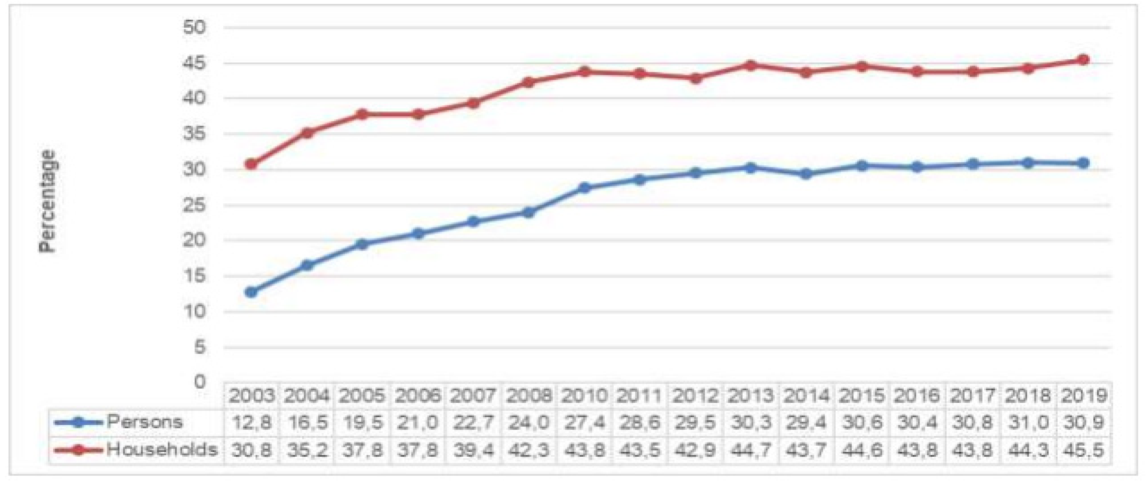
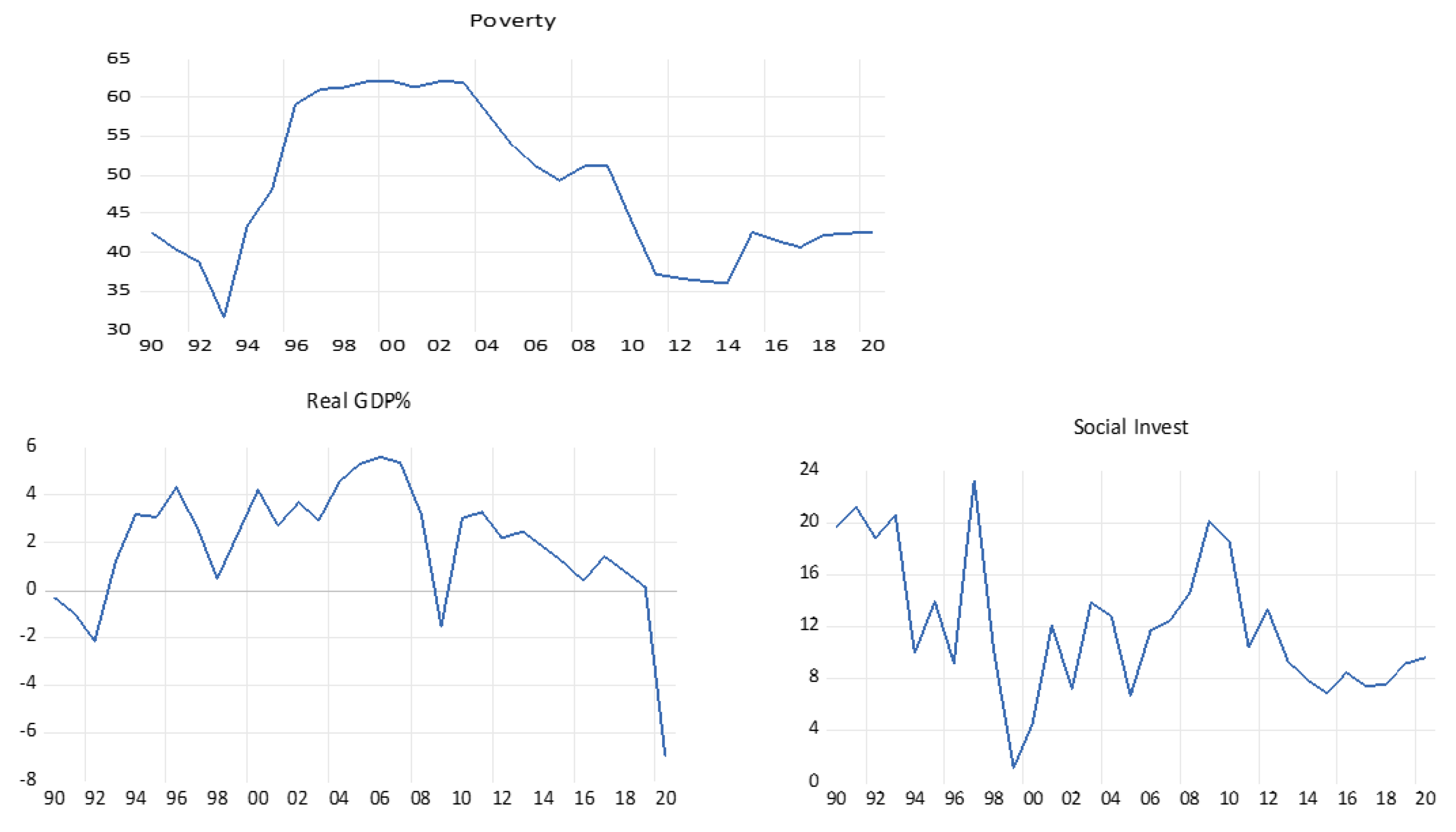
Table 1.
Summary of variables description and expected signs and relationship.
| Variables | Description of Variables | Expected Relationship with Social Investment |
|---|---|---|
| SOCIAL INVESTMENT | Expenditure on social investment is captured as aggregate expenditure on social investment to government expenditure [for instance, education, housing, health, and social services]. This is a proxy for social investment. | |
| POVERTY | Poverty is a measure of the basic standard of living for the citizens of a country. The annual per capita income, the percentage of the population living on less than one or two dollars per day, and the three poverty lines used in South Africa were all proposed as indicators for poverty measurement in the previous literature. | + (positive) |
| GDP | It is proxied for annual earnings, which are captured as domestic absorption in an economy. | + (positive) |
Table 2.
Augmented Dicky-Fuller test at first difference with trend and intercept.
| Variables | Level Test Statistic | First Difference Test Statistic | Critical Values | Order of Integration | ||
|---|---|---|---|---|---|---|
| 1% | 5% | 10% | ||||
| SOCI | 0.8342 | 0.0016 | −4.309824 | −3.574244 | −3.221728 | Non-Stationary I(0) at level form and first difference Stationary I(1) at all critical values (1%,5%,10%) |
| POV | 0.8435 | 0.0008 | −4.309824 | −3.574244 | −3.221728 | Non-Stationery I(0) at level form but first difference Stationary I(1) at all critical values (1%,5%,10%) |
| GDP | 0.8540 | 0.0021 | −4.309824 | −3.574244 | −3.221728 | Non-Stationery I(0) at level form but first difference Stationery I(1) at all critical values (1%,5%,10%) |
Source: Author’s computation.
Table 3.
Cointegration test on Social Investment and Poverty.
| Trace Statistics | ||||
| Hypothesized No of CE(s) | Eigen Value | Trace Statistic | 5% Critical Value | Probability |
| None | 0.265684 | 8.712390 | 15.49471 | 0.3927 |
| At most 1 | 0.002338 | 0.065534 | 3.841465 | 0.7979 |
| *(**) denotes rejection of the claim at the 5% level. Trace test indicates no cointegration at both the 5% level. | ||||
| Max Eigen | ||||
| Hypothesized No of CE(s) | Eigen Value | Max Eigen Statistic | 5% Critical Value | Probability |
| None | 0.265684 | 8.646855 | 14.26460 | 0.3167 |
| At most 1 | 0.002338 | 0.065534 | 3.841465 | 0.7979 |
| *(**) denotes rejection of the claim at the 5% level. Max Eigen value test indicates no cointegration at both the 5% level. | ||||
Source: Author’s computation.
Table 4.
Diagnostic Tests for Social Investment and Poverty.
| Heteroscedasticity | |||
| F-static | 1.486196 | Prob. F | 0.2330 |
| Obs * R-square | 1.512093 | Prob. Chi-square (1) | 0.2188 |
| Scaled explained SS | 0.290785 | Prob. Chi-square (1) | 0.5897 |
| Breusch-Godfrey Serial Correlation LM Test | |||
| F-Static | Durbin-Watson stat | Prob. | |
| 99.97582 | 1.894210 | 0.000000 | |
| Outlier Test for Poverty | |||
| Coefficient | R-square | Probability | |
| −0.901970 | 0.919766 | 0.0028 | |
Source: Author’s EViews computation. *—represents significance.
Table 5.
Cointegration Test on Social investment and GDP.
| Trace Statistics | ||||
| Hypothesized No of CE(s) | Eigen Value | Trace Statistic | 5% Critical Value | Probability |
| None | 0.306706 | 10.25643 | 15.49471 | 0.2615 |
| At most 1 | 4.56 × 10⁻⁷ | 1.28 × 10⁻⁵ | 3.841465 | 0.9992 |
| *(**) denotes rejection of the claim at the 5% (1%) level. Trace test indicates no cointegration at both the 5% and 1% level. | ||||
| Max Eigen | ||||
| Hypothesized No of CE(s) | Eigen Value | Max Eigen Statistic | 5% Critical Value | Probability |
| None | 0.306706 | 10.25642 | 14.26460 | 0.1956 |
| At most 1 | 4.56 × 10⁻⁷ | 1.28 × 10⁻⁵ | 3.841465 | 0.9992 |
| *(**) denotes rejection of the claim at the 5% (1%) level. Max Eigenvalue test indicates no cointegration at both the 5% and 1% level. | ||||
Source: Author’s EViews computation.
Table 6.
Diagnostic Tests for Social Investment and GDP.
| Heteroscedasticity | |||
| F-static | 0.036361 | Prob. F | 0.8501 |
| Obs * R-square | 0.038820 | Prob. Chi-square (1) | 0.8438 |
| Scaled explained SS | 0.097992 | Prob. Chi-square (1) | 0.7543 |
| Breusch-Godfrey serial correlation LM Test | |||
| F-Static | Durbin-Watson stat | Prob. | |
| 6.830415 | 1.543980 | 0.003977 | |
| Outlier Test for GDP | |||
| Coefficient | R-square | Probability | |
| −0.215745 | 0.641184 | 0.0013 | |
Source: Author’s EViews computation.
Publisher’s Note: MDPI stays neutral with regard to jurisdictional claims in published maps and institutional affiliations. |
© 2022 by the authors. Licensee MDPI, Basel, Switzerland. This article is an open access article distributed under the terms and conditions of the Creative Commons Attribution (CC BY) license (https://creativecommons.org/licenses/by/4.0/).
Share and Cite
MDPI and ACS Style
Ogujiuba, K.; Mngometulu, N. Does Social Investment Influence Poverty and Economic Growth in South Africa: A Cointegration Analysis? Economies 2022, 10, 226. https://0-doi-org.brum.beds.ac.uk/10.3390/economies10090226
AMA Style
Ogujiuba K, Mngometulu N. Does Social Investment Influence Poverty and Economic Growth in South Africa: A Cointegration Analysis? Economies. 2022; 10(9):226. https://0-doi-org.brum.beds.ac.uk/10.3390/economies10090226
Chicago/Turabian StyleOgujiuba, Kanayo, and Ntombifuthi Mngometulu. 2022. "Does Social Investment Influence Poverty and Economic Growth in South Africa: A Cointegration Analysis?" Economies 10, no. 9: 226. https://0-doi-org.brum.beds.ac.uk/10.3390/economies10090226
Note that from the first issue of 2016, this journal uses article numbers instead of page numbers. See further details here.