
Dynamic Modeling of Environmental Subsidies


Department of Economics, University of Thessaly, 38333 Volos, Greece
*
Author to whom correspondence should be addressed.
Economies 2024, 12(4), 75; https://0-doi-org.brum.beds.ac.uk/10.3390/economies12040075
Submission received: 26 January 2024
/
Revised: 16 March 2024
/
Accepted: 20 March 2024
/
Published: 26 March 2024
(This article belongs to the Section Growth, and Natural Resources (Environment + Agriculture))
Abstract
:In this research, the intertemporal optimal management of subsidies offered by the environmental regulator and the dynamic conflict between two groups of economic agents involved in environmental quality are discussed. First the environmental model is examined in its optimal control management form with two state variables. The analysis of the improved model, inspecting the social planner’s decision (policy) variable, the variable which influences not only environmental quality but the national budget stock, reveals that is dependent on the growth of the national budget stock. A negative growth rate leads to the long run saddle point equilibrium, while an incremental growth rate, but less than the model’s discount rate, leads to an interesting complicated limit cycle equilibrium, for which under certain parameter values the orbit’s phase portrait can be drawn. For the dynamic game model between the social planner and natural resource exploiters, the equilibrium conditions are examined. It is rather a richer than the point equilibrium for which the cyclical strategies have great importance. Therefore, the conditions for that rich equilibrium are found. As a continuation, the paper concludes that the equilibrium condition is that the players’ discount rates are both greater than the national budget interest rate. Finally, the certain values of the equilibrium strategies and national budget stock are provided.
1. Introduction
Dynamical economic problems can be faced either as optimal control models or as dynamic games. As it is well known, the case of the dynamic games is definitively the -person extension of the case of the optimal control models in which one and only one economic agent coordinates his actions to maximize/minimize his own utility/costs (Dockner et al. 2000). In this paper, attention is given to the special fragment of the national budget stock which is offered by the social planner as a subsidy, while at the same time the group of economic agents that consume the given subsidy is taken into consideration, assuming they do not cooperate with the social planner. Each of the above economic agents, i.e., the social planner and the group of subsidy consumers, chooses his own policy to maximize his own intertemporal discounted utility. Since the subsidy offered is dependent on the national budget, the strategies which are chosen by the players affect not only the levels of the utility of every player but also the common level of the national budget stock. The implications of the latter formulation are as follows (Grass et al. 2008). First, the strategies chosen by the economic players of the game have great implications for the size of the capital stock, i.e., the national budget, which in turn has impacts on the economic magnitudes of any nation. Second, since the game is non-cooperative, the players do not coordinate their movements with each other, but play in a strategic way. Third, according to the game-theoretic view, the result of equilibrium hinges upon the spaces of the available strategies of the players.
According to the information structure followed by the model under consideration, the players of a dynamic game have some actions to choose from, i.e., to define the type of their strategies (Wirl 1997). One type of strategy is that which uses the minimum of information and is based on time alone over the whole horizon of the game played, which is called the open-loop strategy. On the other extreme, closed-loop strategies are strategies in which every player of the game adapts his actions according to the current state of the game.
Supposing that the subsidy’s consumers use open-loop strategies, the only action that they have to do is to fix their trajectory of consumption and adhere to that specific orbit over the entire planning horizon, starting from time zero (Berck 1981). Similarly, if the social planner follows the open-loop policy pattern his only task is to plan a subsidy offering policy at the initial time of the game and stick to that policy until the end of the game.
On the other hand, the adoption of feedback strategies requires the players of the game to adapt the time paths of their offering and consuming activities according to the current state of the stock of the national budget for the whole time horizon of the game (Clark 1990; Clark and Munro 1975). Feedback strategies take into account the interactions among the players in a dynamic game. If a group of subsidy consumers today eats all the subsidies offered, a fact which lowers the level of the national budget stock, the social planner plans their future actions taking into account this instantaneous change in the national budget stock. This is the rationale that the closed-loop strategies are sensitive in the strategic interactions among players (Hartman 1963).
As is well known, subsidies are faced like public expenditures (Gordon 1954; Hannesson 1983), therefore they are financed from the national budget. In turn, whenever a subsidy is offered, there must be taken an equivalent measure, like taxes or like another source of public revenue, in order to balance the national budget. The offer of subsidies is not without justification and, in conclusion, the choice to offer or abolish a subsidy is a result of not only social but private comparison among benefits, costs, and revenues (Plourde 1971; Schäfer 1994). As it became obvious, the subsidy mechanism tends to connect the returns between the private and public sectors in such goods and services in which the observed externalities are very large.
Some examples would be the subsidies in social health, e.g., inoculation against communicable diseases, in education, and especially in the sustainability of the environmental amenities, e.g., sustainability of renewable and nonrenewable resources, social forestry, and water conservation (Liski et al. 2001).
A major problem faced by the government is related to the sustainability of the fiscal deficit. To be more precise, in the case that the very large fragment of subsidy is financed by borrowed funds and not by government income, then the fiscal deficit is exploding, and therefore its time path becomes unstable. As a result, the main purpose of the subsidy mechanism fails, and therefore has the opposite effect (Levhari and Withagen 1992).
The novelty of the present study is how the fiscal policy, i.e., the subsidies of a country, are interrelated with the environmental policy intertemporally in a dynamical way. The latter is based in the economically acceptable dynamical methods, which are the optimal control theory and the game theory. In other words, the main concern, and therefore the novelty of the paper, is how the two economic concepts, subsidies and environmental quality, are interrelated not only in a dynamical way but intertemporally. The game theory approach gives some interesting policy implications that are illustrated during the model analysis in the main text of the paper.
This research extracts three major results. The first refers to the cyclical strategies which have been introduced in dynamical economics only in recent decades, due to the works of Feichtinger and Sorger (1986) and Wirl (1992), with these authors being only a few from along catalog of authors. Furthermore, the meaning of cyclical and more general complex policies has received increasing attention in the last few years as related to overall economic activities. For example, cyclical policies can be found in demand–production models, in business models, in rational addiction economic models, and so on. A cyclical policy or strategy is the result of a limit cycle dynamic equilibrium, i.e., a richer equilibrium than the point equilibrium, and therefore more important. This, in a simple way, implies that a cyclical strategy, because of its oscillation in a certain basin of attraction, sooner or later will retrace its previous steps.
The first result of this study (Proposition 1) is a novel and important interconnection of environmental economics and financial economics, finding the necessary conditions for cyclical strategies between social planners and natural resources exploiters. This condition involves the discount rates of the two players, and therefore the risk premium between the two policies. The second result (Proposition 2) provides the validity of the general model and interconnects environmental economics with fiscal policy in the linear form of the model, involving the discount factors of the two players which are compared with the rate the national budget grows. In our opinion, Proposition 2 is of great economic importance in both environmental and fiscal policies. Finally, the third result (Proposition 3), although computational, provides the exact expressions of the followed policies by the two players of the game in terms of the model parameters. Additionally, it offers the steady state value of the national budget stock, again an important interconnection with the fiscal policy.
According to the modeling of public debt as an accumulated variable (Halkos et al. 2020), budgetary resources, which are offered as subsidies, can be thought of as an inseparable crucial part of the public debt, and therefore can be treated as an accumulated variable. For the above variable, which is treated as a decision variable, any instantaneous change is dependent on the most recently approved subsidy and its historical adjustments. To the best of our knowledge, this is a novel assumption in the economics of environmental subsidies, which is governed by intertemporal rules, since any subsidy offered is the result of historical approvals or withdraws.
This research aspires to contribute to the existing literature on both points of view of the subsidies problem, i.e., first in the dynamic management model and second in the dynamic conflict of the subsidies problem. This study continues the novelty of modeling in which subsidies are managed as a function of the accumulated national budget, extending a model that has been introduced by (Halkos et al. 2019). Moreover, this research extends the modified problem in a Nash dynamic game in which the conditions between the discount factors of the players for the limit cycle equilibrium are found.
The structure of this study is as follows. The relevant literature review is presented in Section 2. Some useful comments on how a connection between the management of subsidies and cyclical economic actions are made in Section 3. The extension of the one-state model in the two-state model is introduced in Section 4. In Section 5, the differential game model and its limit cycle equilibrium are analyzed. In Section 6, the findings of the paper are discussed, while the last Section concludes the research.
2. Literature Review
The proposed model is an extension of a previous model by (Halkos et al. 2019), not only concerning its setup but also in the way the environmental subsidies conflicts are considered. In this paper, the authors propose a dynamic optimal control theory model of environmental subsidies in which environmental quality is maximized in the infinite planning horizon, under two certain and sufficient constraints; i.e., first, the national budget constraint which is described by the differential equation of its instantaneous change, and second by the historical adjustments of the subsidies decision which in turn is described by a corresponding differential equation as well. As a result, the authors give sufficient policy implications in order for the credible cyclical strategies to apply. Another crucial result for environmental policy, extracted by the same paper, involves the discount rates of the policy maker and the opportunity cost of the environmental capital. As a result, since the discount rate is less than the opportunity cost, the optimal policy is currently preferred to be a taxation policy, related to environmental taxation on clean technologies reducing carbon emissions and also green financial instruments of cleaner production technologies. These policies will allow for future subsidies.
Another paper related to environmental quality is (Halkos and Papageorgiou 2021). In this paper, the authors propose two game theoretic models according to dynamic Nash and Stackelberg issues of equilibrium. Both players of the games havet heir own (different) strategies and a common state variable, concerning environmental quality, which is the volume of emissions generated by the polluting firms. A major conclusion of the paper, comparing the two types of equilibrium, is that the conflict between the two players of the game, i.e., the social planner and the polluters, is more intensive in the Stackelberg case, concluding with the exact expressions of the extracted strategies.
In another view, and in another paper by Halkos and Papageorgiou (2018), a game theoretic model between the social planner and the polluting firms is applied in order to examine the environmental causes in public debt, and therefore in the subsidy mechanism. The results of their proposed models are robust for the policy makers in both Nash and Stackelberg cases, as follows: First, in the Nash setting, the condition for the credible cyclical strategies is that the government is more farsighted than the polluters. Second, in the Stackelberg case with the polluters as the followers of the game, the authors found (a) the model parameter values for which there exist a feasible solution, (b) the analytical expressions of the strategies for both players, and (c) the range of the parameter values for which the social planner acts more cautiously and the polluters more aggressively compared to the Nash case. In both cases, the results suggest certain policy proposals, in our opinion.
Some other aspects of the environmental problem of degradation can be found in a paper Kwakwa et al. (2018) in which the Environmental Kuznets Curve (EKC) hypothesis is examined empirically with evidence from Tunisia. In their paper, a comprehensive analysis was conducted to understand the potential existence of the EKC hypothesis for various sources of CO2 emissions within the context of financial development and natural resource extraction in Tunisia. They conclude that CO2 emissions emanating from the consumption of solid fuel would eventually increase as the Tunisian economy grows larger.
Another paper related to methodology used in the first part of the proposed model is (Leventides et al. 2022), in which data-driven and machine learning methods from the theory of Koopman operators and Extended Dynamic Mode Decomposition are applied in the study and analysis of the business cycles. Such techniques are extensively used in dynamical systems and control theory, especially in the case of non-linear or unknown dynamics. Their primary purpose is to approximate the two-dimensional, non-linear model with a linear dynamical system which will be able to capture the main features of the business cycle and it will be more suitable for prediction and control. The paper results exhibit that following their approach gives good approximation results if one considers one trajectory and a finite time horizon in this realistic scenario.
3. An Intuitive Explanation of the Cyclical Actions between Subsidies and Environmental Exploitation
The optimal growth model proposed by Skiba of the one-sector economy, for which the production function is convex–concave (Skiba 1978), was the cornerstone of the economic literature regarding cyclical strategies as solutions in dynamical economic models. A great example would be Wirl’s model (Wirl 1995), which extends the former renewable resources model of (Clark 1979). Wirl’s conclusion is that the cyclical strategies of extraction are admitted as equilibrium policies even in the case at which the equilibrium points range between the intertemporal rule of exploitation and the maximum sustainable yield.
This paper aims to discuss the oscillatory behavior implied by the solution of the dynamical system of the proposed model, using limit cycles and, especially, the stable version of the cycles. Since, as is intuitive, any orbit of a dynamical system has as a basin of attraction a closed and bounded subset, and with time passing has to retrace its previous steps (Kuznetsov 2000). Translating this into policies, a subsidies policy that offers or abolishes subsidies, and moreover is bounded by the restriction of the national budget, sooner or later has to follow a specific one of its previous trajectories.
When higher than two dimensions, the sufficient condition for the existence of stable limit cycles is not only the existence of a pair of imaginary eigenvalues, but the first derivatives of the associated real part of the same eigenvalues are also involved. More specifically in the case of , the dimensional system is tuned by a parameter , having also an isolated equilibrium point , implying that the condition for Hopf bifurcations is the following: an existing simple pair of complex conjugate eigenvalues to cross the imaginary axis from left to right, while the other eigenvalues have negative real parts (Manfredi and Fanti 2004).
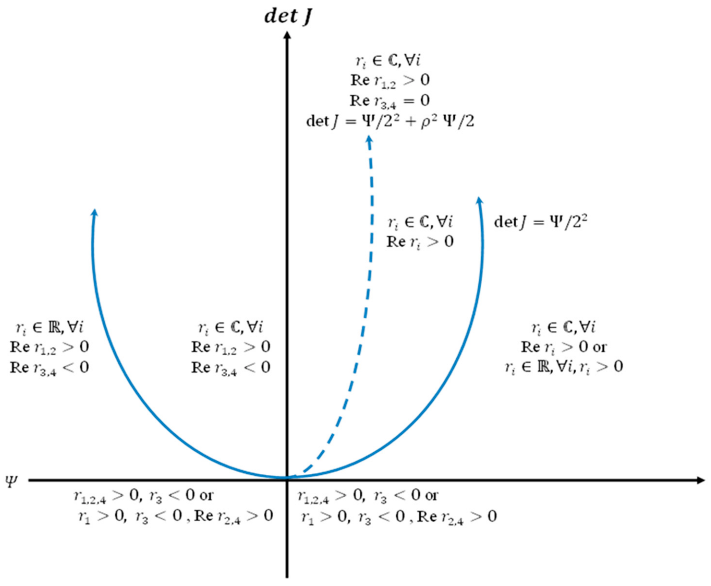
Figure 1 is based on Lemma 2 of Dockner and Feichtinger (1991) and distinguishes the set of conditions which fully characterizes the local stability properties of the dynamical system of Equations (10)–(13) in the main text. The involved expressions and Ψ are given in the main text by Equations (15) and (14), respectively. The dotted curve (bifurcation curve) and the parabola separate the space in the following five regions.
- Region 1: In the left of the leftmost branch of the parabola and upper of the Ψ axis.
- Region 2: Between the leftmost branch of and the curve .
- Region 3: Along the bifurcation curve .
- Region 4: The right space of the bifurcation curve and upper the Ψ axis.
- Region 5: Down the Ψ axis.
According to Figure 1, we expect four dynamic types of behavior. For regions 1 and 2, we expect saddle point stability of the above dynamic system, complete instability for the region 4, the existence of an one-dimensional stable manifold in region 5, and the existence of closed contours with the possibility of limit cycles along the bifurcation curve in Region 3.
In economics, bifurcations are of great importance, mainly because they are the outcome of the interactions between endogenous non-linear forces. Such interactions could be, according to (Dockner and Feichtinger 1991), the cross effects of capital stocks and the positive growth of some economic magnitudes.
An intuitive explanation of cyclical policies in the below environmental subsidies, between the economic agents involved in environmental exploitation activities and the government, could be the following. The people who are interested economically in the exploitation of natural resources enjoy utility stemming from the higher intensity of their extraction mechanisms, while the opponent, i.e., the social planner, gains utility from the higher level of the restored environmental quality as a result of the subsidies offered (Ströbele 1988; Ströbele and Wacker 1995). The starting point is a low and declining national budget. Since the social planner benefits from a higher possible rate of subsidies, the offer must increase the national budget up to the point at which the marginal increment would cause high unfavorable costs. Because of the national budget increment, the rate of the given subsidies is incremental, and therefore the exploiters of environmental resources intensify their exploitation actions. The latter actions would tend to stabilize the dynamic system towards the steady-state. A realistic assumption is adopted that the exploiters of environmental resources behave myopically, and therefore they accelerate the rate of their economic actions. The social planner who cares about environmental quality reacts by an incremental abolishing of subsidies. In order to avoid the loss of the previous amount of subsidies, the exploiters of environmental resources have to incrementally decelerate their extraction rate, and at that time the cycle of actions and counter-actions would close.
4. The Extended Subsidies Management Model
The research methodology used is clearly dynamical economics methodology, specifically the optimal control and differential games theories. Concerning the management model, this could only be treated dynamically and one of the appropriate tools for that analysis is the optimal control theory. In the same way, as a continuation of the management model, the most credible tool which favors the analysis of the conflict between the persons involved in environmental degradation and restoration, bearing in mind the historical nature of the subsidies decision, is the dynamic (differential) game theory. The choice to describe the clash between the two rival sides of the environmental model as a differential game is not only because of the conflicting nature of game theory but also because of the intertemporal nature of environmental resources as capital.
In the classical stock literature, someone can consider the management of the subsidies taken from the national budget as a stock model of two state variables; one variable could be the national budget and the second could be the subsidies offered in order to improve the environmental quality (Halkos et al. 2019). In that primitive case, the above optimal control model, with adjustment costs, is written as:
Subject to
where is the utility function enjoyed by the social planner, is the subsidies function, and the national budget, while is the cost function due to the adjustments in environmental quality, is the growth function of the national budget, and is the state of environmental quality. This model admits saddle point stability in the case at which the national budget growth function has the form of the increment logistic function, and moreover the conditions and are met (Halkos et al. 2019).
The basic two-dimensional model (1)–(3) is extended, taking the subsidies as an amount which shrinks or augments.
The decision for increment or decrement of the overall subsidies is also significantly depending on the current instantaneous environmental quality rate; therefore, the overall amount of the subsidies might be taken as a stock, which straightforwardly impacts the total subsidy function (Farmer 2000; Halkos and Papageorgiou 2014). However, since the subsidy function is a function dependent on environmental quality, this is denoted by . Environmental quality , does not remain at a given state, but deteriorates with a simple depreciation rate. Additionally, it is obvious to mention that the central manager of subsidies enjoys utility from his decision to restore environmental quality. If the social planner handles the environmental quality as a variable that denotes the state parameter, the choice to offer or abolish a subsidy would be the new control variable which is incorporated in the system.
With the above assumptions, the optimal control problem (1)–(3) might be modified as below:
Subject to
where is the total utility applied in a separable form, i.e., the sum of the utility originated from the existing national budget stock plus the utility stemming from the social’s planner decision . The subsidies function can be expressed as a function of the expected environmental quality, while illustrates the depreciation rate of the environmental quality. The control (policy) variable influences not only the changes of environmental quality in a direct way, but also indirectlyaffects the budget stock through the subsidies function . The utility function’s separable form representation illustrates the intertemporal trade-off between the profits linked to the higher national budget and the advantages stemming from environmental quality improvements, (Halkos and Papageorgiou 2014). The assumption that inside utility is embodied in all the costs associated with the management of environmental amenitiesis used. Finally, the policy about environmental quality, , may be positive in the event of improvement or negative in the occurrence of deterioration. The latter states that the depreciation factor, in the steady state equilibrium, can be set to zero, which in turn implies that , i.e., no changes are made in environmental quality.
The optimal control problem under the constraints (5) and (6) is solved as follows.
The Hamiltonian is:
where are the adjoint variables of the states respectively.
The concavity of the Hamiltonian function, both on state variables as well as on the control variable, of the problem under consideration, together with the transversality conditions, are exactly adequate circumstances for the optimality of the control issue. The limiting transversality conditions are listed below:
Next, the maximizing condition of the Hamiltonian for the control values is given by
And taking into account the concavity of the Hamiltonian, then
Taking the inverse function (which already exists), the above optimality condition is satisfied:
The co-state variables evolve according to the following equations of motion:
Now the construction of the so-called canonical system of the necessary conditions follows. This system is constituted by the Equations , , and , i.e., the system described below:
with the following Jacobian matrix:
In order to compute the eigenvalues of the Jacobian matrix it is simple to apply Dockner’s formula (Dockner 1985). Note that the four eigenvalues of the Jacobian matrix are used to distinguish the linear system’s approximation (10)–(13). Applying the formula of the four roots are gives
where
Making the appropriate substitutions the coefficient of the formula reduces in to
while the determinant of the Jacobian reduces into the following expression:
Assuming that an interior solution exists for the concave problem – then the system’s stability properties, which are mostly determined by the sign of the growth function’s rate of change, i.e., on the sign of , are derived, which are also dependent on the other qualitative characteristics of the model as noted below.
Case 1:, according to , since , then and . As a result, two of the eigenvalues require negative real parts and consequently the long-run equilibrium is a saddle point.
Case 2: . The long-run equilibrium can be described by all different cases, i.e., saddle point stability and locally volatile spirals, and destabilization because of the converge to equilibrium is limited to a one-dimensional set of initial conditions. Based on the Poincare–Andronov–Hopf (PAH) theorem (Kuznetsov 2000), the shift from a stable domain to a locally unstable one may give rise to limit cycles.
Supposing that there is growth, , and a process of diffusion with a single and unique budget point such that , it is widely understood that the temporal path of the budget level is made of a convex segment and a concave segment (if ). To put it another way, the domain of the low level illustrates increasing returns and the domain of the upper level is characterized by diminishing returns. It is feasible that declining returns result in a stable equilibrium, whereas increasing returns favour complicatedness, i.e., limit cycles. The rationale for this is that a small percentage of the national budget may climb to a particular point, making it sensible for the agent to develop his equipment in order to receive future advantages.
Specifications
Advantages are anticipated from the national budget stock proportionate to its current condition. Furthermore, the expansion of advantages connected with the existing level of environmental amenities, however, is not unbounded, but rather approaches a limit. Thus, the functional forms are defined as below:
The last two formulae express the notion that there is a budget ceiling that must be met, which rises when there is lack of subsidies, whereas the diminution of the budget’s level grows in proportion to the total amount of environmental quality . Nevertheless, because of the large depreciation that has been made on the previous accumulated environmental quality, the decision for adjustments has a very minor meaning in the long term. In other words, at the steady state, the choice of , drops to zero and this outcome is only possible if the depreciation rate is set close to zero, . With this final assumption, and under the requirements (17)–(20), the determinant of the Jacobian along with the coefficient reduces into
Having the set of requirements for the presence of a pair of entirely imaginary eigenvalues, i.e., , and , the bifurcation point is kept for the specific parameter values , ,. It can be demonstrated quantitatively (Grass et al. 2008) that the criteria for complex eigenvalues with positive real parts are fulfilled for the aforementioned parameter values , and furthermore there are stable limit cycles, at least in the right-hand proximity of (Halkos and Papageorgiou 2014).
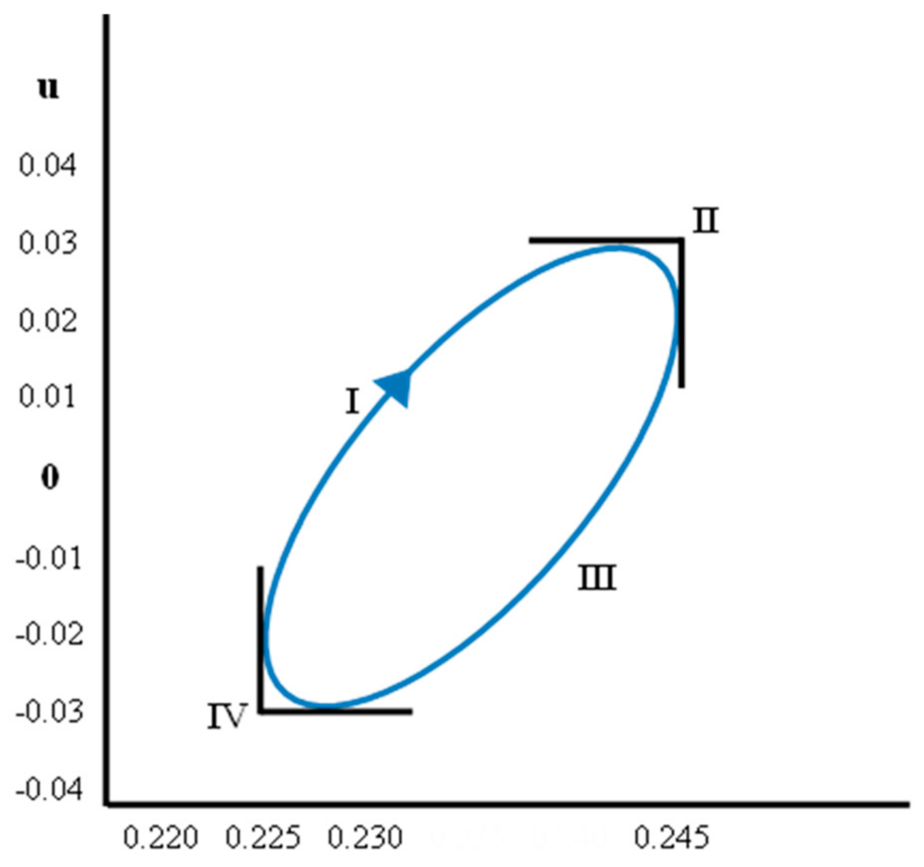
The phase portrait in the modification–stock plane is depicted in Figure 2, which corresponds the aforementioned values of .
5. Conflicts with a Shared Function of Subsidies
Based on the assumption of the previous section, the instantaneous budget is presented by and has common access at time . The budget grows based on the function , having no subsidy taken into account, undoubtedly on the basis of the budget itself. This happens by the satisfaction of the following conditions: for all , for all , . For the following game, it is assumed that two types of players are involved. The first player is the social planner who cares to maintain the amenities of the environment. The second player is the commercial heavy equipment extractor of environmental resources acting as factories. Regarding the second type of player, it is costly to carry out the exploitation of environmental resources; examples of costs include (i) damages to the available equipment, (ii) payroll for employees, and (iii) diminution of financial capital (Halkos and Papageorgiou 2014). Taking into account the process of depletion of the budget stock (the environmental subsidies function) does not only rely on frequent usage of the heavily equipped exploiter but is also influenced by the environmental restoration effort undertaken by the other player, i.e., by the effort of the social planner. As instrument variables, the intensity of their extracting actions and the planner’s effort are respectively established, meaning (i) the intensity of the extracting equipment’s usage for the heavily equipped player (player type 2), and (ii) the effort for the social planner (player type 1) are both assumed to be non-negatives .
The subsidies function is stated by , which depends on both the planner’s effort and the intensity of the extractors. Bringing together the growth with the subsidies function , the state dynamics can be expressed as
The non-negativity constraint is imposed along a trajectory, that is
As intensity from the perspective of player 2 rises regarding the extracting equipment utilization and as the effort from player 1 (i.e., the social regulator) rises as well, these two actions usher in a certain stronger depletion of the national budget via the use of subsidies. Hence, it is reasonable to believe that the partial derivates of the subsidies function are positive with respect to the parameters, i.e., (Halkos and Papageorgiou 2014). In addition, the type 1 player’s effort is affected by the law of diminishing returns, which is , or it might be assumed that in order to make it simpler. Moreover, the assumption that the Inada conditions remain true(guaranteeing the non-negativity of the optimal strategies) is made, i.e.,
The two players want to maximize the following utility functions: Player 1 (i.e., the social planner) desires instantaneous utility, firstly from its own subsiding program, but its actions stimulate increasing and convex costs , and secondly from the high stock of budget also stated by the increasing function .
Bearing in mind the previous assumptions, the present value of player 1’s utility is defined by the following functional.
Player 2 (i.e., the extractor of natural resources) benefits from utility for two reasons: (i) the existing national budget stock and (ii) their extracting actions usage intensity , which can be presented by the function . Regarding the utilities and , it can be assumed that they are monotonically increasing functions with decreasing marginal returns, meaning that and . It can be further purported that the social planner’s overall effort has zero effect on player 2’s utility. Hence, player 2’s utility function can be given, in additively separable form, as
The methodology used in the proposed model undoubtedly includes not only the heavily equipped exploiter but every type of extractor of natural resources (renewables or non) starting from a simple fisherman, a simple miner, etc., to a heavily equipped industry of extraction. The notion “heavily equipped exploiter” is only used in order to give some emphasis, as a representative agent, but the model is applicable for all types of natural resources extractors, since the same utility function (27) is applied for all types of exploiters of natural resources.
5.1. Periodic Solutions
In the subsection that follows, the stability and steady state analysis of the important conditions of the model is carried out, which is considered as a differential game that contains two controls and one state variable. Corresponding Hamiltonians, optimality conditions, and adjoint variables for the problem under consideration are, respectively,
The subscripts state player 1 and player 2 for Hamiltonian , respectively, and the adjoints . The solutions of the system of equations are the steady state solutions for the state, the adjoints, and the controls:
The following matrix denotes the Jacobian matrix referring to the system of optimality conditions:
which also gives the following: trace, , and the determinant, as
and
Based on (Wirl 1997), the satisfaction of the following conditions demand the existence of a pair of purely imaginary eigenvalues:
where the result of the sum of the following determinants is coefficient .
It is important that the crucial condition for cyclical strategies be defined in order to have Hopf bifurcations occur, which can be stated as
After simple algebraic calculations, this becomes
5.2. Specifications for the Game
The game’s functionalities are defined as follows: a diffusion technique for budget function expansion, that is , a Cobb–Douglas type function for the subsidies function , and the utility function resulting from player 2’s equipment use intensity as in the equation . Observing that the utility function with and presents constant relative risk aversion in the sense of the Arrow–Pratt measure of risk aversion (Pratt 1964; Halkos and Papageorgiou 2014), the rest of the functions remain in a linear form. This means that the utilities deriving from the existing budget stock are for player 1 and for player 2 , while player 1’s effort cost is in the linear fashion as well, observing that all the included coefficients, i.e., the intrinsic growth rate and the slopes , and , are positive real numbers, but ,, and as already mentioned (Halkos and Papageorgiou 2014).
Having in mind the above specifications, the following outcome holds true.
Proposition 1.
A necessary condition for cyclical strategies in the game between the social planner and the exploiters of the environmental resources, as described above, is the exploiters of the natural resources take riskier actions compared with the social planner.
Proof.
See Appendix A. □
The insight behind Proposition 1 is apparent. Beginning with a rather low and increasing intensity of the actions undertaken by the exploiters of environmental resources, the intensity of the actions is represented by the control variable . The social planner operates at low effort as well, because the higher the increasing effort, the higher the costs. Furthermore, the social planner is worried about the budget level, considering the environmental quality, amplified by the intensity of the actions undertaken by the environmental exploiters. Under the assumption that the exploiters react in a farsighted way, the social planner might raise the intensity of equipment only slightly, leading the dynamical system to a stable steady state.
Nevertheless, accounting for their impatience, the exploiters behave myopically and react by robustly increasing the magnitude of their activities. This leads the social planner to choose between leaving the environmental quality deterioration or increasing the overall effort through the subsidy mechanism. Supposing that the social planner increases the subsidies devoted to environmental quality, this might lead to a combination of high intensity on behalf of the exploiters and an even higher effort (i.e., subsidies) on the planner’s part, ultimately resulting in a high diminution of the national budget stock.
However, the low standards of the national budget stock (and therefore the low level of subsidies) are unprofitable for the exploiters of environmental services to operate at great magnitude, leading them to decrease intensity on their part and the cycle would close.
The beginning of a new cycle happens again, probably at a different level due to the budget stock’s reduction, nevertheless following the same described results. Our thoughts are that the crucial point of this intuitive description is that the strategic variable of the first player lags behind the strategic variable of the second player, and both lag behind the state variable, the national budget stock .
5.3. An Example of the Game
The present subsection includes our calculation of the Nash equilibrium regarding the subsidies differential game. The notion of open-loop Nash equilibrium is based on the assumption that every player’s strategy can be deemed as the best reply to the opponent’s exogenously-derived strategy. Hence, it is apparent that equilibrium happens if both strategies are simultaneously the best replies (Halkos and Papageorgiou 2016). Based on (Dockner et al. 2000), the formulation of the current value Hamiltonians for both players, is as below:
The first order conditions, for the maximization problem, are the following system of differential equations for both players.
First, the maximized Hamiltonians are
and second the costate variables are defined by the equations
The Hamiltonian of player 1, , is concave in the control as far as and is guaranteed by the assumptions on the signs of the derivatives, i.e., and from the decreasing marginal returns on player 2’s utilities, i.e., (Halkos and Papageorgiou 2016). Moreover, the optimality condition indicates that the adjoint variable takes positive values only if player 1’s marginal utility exceeds the marginal costs, since .
Linearity of the model is also assumed. A linear growth function, despite the critique as a fairly unrealistic model, is a good approximation for the exponential growth of the budget since the 19th century (Murray 2002). To be more precise, the game’s subsequent functions are expressed in linear form:
- The growth function of the budget in the form , where is the interest rate;
- The utility function, , which stems from the high stock of the budget, in the form ;
- The function that measures player 1’s effort cost in the form .
All of the constants are positive values, that is, . For the second player’s part, the maximized functions are linearly specified, i.e., the utilities derived from the budget stock and high intensity realizations are written as and , respectively.
Following the above-mentioned improved specifications, the canonical system of Equations (33)–(36) can be rewritten as follows:
and the limiting transversality conditions must hold:
The analytical expressions of the adjoint variables , solving Equations (39) and (40), respectively, are:
In order for the transversality conditions to be fulfilled, it is simple to select the constant steady state values; thus, the adjoint variables are rendered to the following constants:
Wanting to assure certain signs for the adjoints (44), another condition on the discount rates has been imposed by our part, which demands that discount rates are greater than the interest rate, i.e., the proposed condition is:
Thus, the constant adjoint variables both have positive signs.
Considering the inexistence of other optimal solutions, the above restrictive condition is justifiable. Indeed, by choosing , player 2’s discount rate is lower than the interest rate, and their objective function becomes unbounded in the case that they choose to carry out no exploitation (Halkos and Papageorgiou 2016). In a similar way, by selecting player 1’s discount rate to be slightly lower than the interest rate, the associated adjoint variable eventually becomes a positive quantity. As a shadow price is implausible to be positive for optimal solutions, the aforementioned argument is satisfactory for the assumption . The above discussion is recorded as the next result.
Proposition 2.
The proposed game in its linear form admits a solution only if the discount rates of both players are greater than the interest rate at which the national budget grows.
Having the concavity of the Hamiltonians fulfilled in relation to the strategies for each player, the first order conditions assure its maximization. Next, the specification of the subsidies function that reduces the budget stock is selected. This specific function depends on effort and as well as intensity. A production function similar to the Cobb–Douglas specification is chosen that can be characterized by constant elasticities, withthe form:
The next subsection is dedicated to the calculations of the explicit formulae at the Nash equilibrium.
5.4. Optimal Nash Strategies
Applying first order conditions for the chosen specification function,
Combining Functions (45) and (46) using the Cobb–Douglas type of specification unveils an existing interconnection between the strategies, that is,
The interconnection between the players’ Nash strategies can be now predicted by Expression (47). The interconnection of these strategies is dependent on the constant parameters and on the constant adjoint variables as well.
The substitution of (47) into (46) provides significant information about how to find the analytical expressions of the strategies. Expression (46), after evaluating the below algebraic calculations, becomes:
Based on the above, the analytical expressions for the equilibrium strategies can now be expressed in a more comparable form:
Further substitutions in the equation of resource accumulation, , yield the following steady state value of the stock:
The above discussion is summarized in the proposition that follows.
Proposition 3.
If it is assumed that the subsidies function exhibits constant elasticity, then the environmental quality game with subsidies yields constant optimal Nash strategies. The analytical expressions of the strategies are given in Expressions (48) and (49) for the social planner and the exploiters of the environment, respectively. The steady state value of the national budget stock is given by Expression (50).
Proposition 3 seems to have little economic meaning, caused by the linearity of the paradigm. However, the constancy of the resulting strategies can be seen in connection with the concept of time consistency, a central property in economic theory. In fact, time consistency is a minimal requirement for any strategy’s credibility, but in general, the open-loop strategies do not have (by definition) the time consistency property since these strategies are not functions of the state variable but are, rather, time dependent functions. Nevertheless, a constant strategy may be a time consistent one, since the crucial characteristic for time consistency, i.e., the independency of any initial state B0, is met for the above constant strategies.
6. Discussion
Examples of subsidy mechanisms could be taken from education. If long-term structurally unemployed workers gain useful training and education, it enables them to find work. This has benefits for other people in society. The government receives more tax revenue and pays less unemployment benefits. There is also a less tangible benefit of a more cohesive society. A second example is that taken from health care. Free universal health care can ensure everyone gets vaccinated; this prevents the spread of infectious disease, which benefits everyone. In other words, an individual has a personal benefit from other people being healthy.
The results of the proposed models are fully applicable in all cases of environmental resources exploitation, such as renewable and nonrenewable resources. Since the crucial variable which interconnects the utilities of the model maximized the with subsidies function is a generalized environmental quality function, the proposed model covers and is applicable to all types of natural resources, both renewables and non-renewables.
Concerning the results of the proposed models, comparing with the results of a previous study involving subsidies as an improvement measure of environmental quality, these results bring cyclical equilibrium strategies one step forward. More precisely, for certain values of the bifurcation parameter, there exists a limit cycle equilibrium, at least in the right-hand proximity of that parameter.
Since the two proposed models, optimal management and game theory, involve social planning, in both cases the extracted results are by default economic policy implications. Taking the social planner’s position, one policy implication could be that the optimal cyclical policy regulation should be that the movements of the regulator are less impatient compared with the opponent players, i.e., an optimal policy for the social planner should be less risky. A second policy implication can be proposed that the discount rate of the social planning must to be greater than the interest rate the social budget grows. A third policy implication is that the social planning should be in a position to predict the resulting policies of a potential game between the government and the rivals, and this could be done only in the proposed case in which the functional forms of the two policies are rigorous expressions (Expressions (48) and (49) in the main text).
7. Conclusions
In the field of stock economics, the national budget stock is a frequently overlooked field. As it is widely understood, the analysis centers around the two primary elements that influence the national budget; specifically the size of the budget itself and the rate of subsidies offered in order to sustain environmental amenities. The afore mentioned specification does not take into consideration any other subsidies that impact the national budget, for instance, subsidies for poverty.
Regarding long-run equilibrium, commonly recognized as the simplest case of saddle–point type stability, only one attribute is required of the growth function of the national budget, meaning negative growth. However, even if the assumption of negative growth is adequate for saddle-point stability, local monotonicity is not assumed, meaning that transient cycles could arise.
Nonetheless, subsidy management is not only limited to the traditional view of environmental quality from the perspective of the social planner. Ensuring the sustainability of the environmental quality often requires subsidy variation, i.e., the reduction or augmentation of the subsidy amount offered, and the undertaken decision about expansion or reduction obeys the state variable which is the existing budget stock. Moreover, regarding the national budget as the stock variable, equilibrium dynamics get more complicated, and much wealthier, also including saddle-point stability. In the discussion in this paper, the dynamics of such equilibrium dynamics present cyclical policies as optimal strategies, but from the above discussion, only some conclusions have been drawn.
The present research’s emphasis is not only limited to the stability properties of the optimal management program, but also there are stability aspects of the induced non-zero-sum game between two categories of players that share a common subsidies function are the subject of this paper. Particularly, the game setup between the social planner and the group of environment exploiters with a common subsidies function yields an economic outcome, where the discount rate has a significant impact on periodic solutions. The prerequisite for periodic solutions is that the exploiters be well-equipped, with impatience greater than the social planner. Finally, for the supplemental linear example of the same game, the optimal Nash strategies for both players are computed, which are constant expressions, and are therefore time consistent strategies.
A limitation of the paper is associated with the proposed game model example, which lies in the linearity of the utilities of the two players, stemming first from the budget high stock and second from the high intensity of exploitation realizations. Another limitation could be the linearity of the growth of the national budget. The utility and the growth functions are left in linear forms without any loss of generality of the model, while in a future paper attention will be given to tackling more generalized functional forms for both growth and utilities. The current proposed models refer to the actors directly consuming these subsidies, and it will be worth exploring the associated indirect effects.
Author Contributions
Conceptualization, G.E.H., G.J.P.; Methodology, G.E.H. and G.J.P.; Validation, G.E.H., G.J.P., E.G.H. and J.G.P.; Writing—original draft, E.G.H. and J.G.P.; Writing—review & editing, G.J.P.; Supervision, G.E.H. and G.J.P. All authors have read and agreed to the published version of the manuscript.
Funding
This research received no external funding.
Informed Consent Statement
Not applicable.
Data Availability Statement
Data are contained within the article.
Conflicts of Interest
The authors declare no conflicts of interest.
Appendix A
Proof of Proposition 1.
Combining (A1) and (A2), the optimal strategies take the following forms:
and the optimal subsidy becomes
with the following partial derivatives
Both derivatives (A6) and (A7) are negatives due to the assumptions on the parameters and on the signs of derivatives, i.e.,
which ensures the positive sign of the adjoints .
Condition now then becomes
which, after substituting the values from (A6) and (A7) and making the rest of algebraic manipulations, finally yields (at the steady states).
where it has been set as stemming from the adjoint equation , which, at the steady states, reduces into .
Condition after substitution the values from (A6) and (A7) becomes
The division (A8) by yields
The sum of (A9) + (A10) must be positive, thus after simplifications and taking into account that , we have
and the result follows from the strict concavity of the logistic growth .
Since the discount rate of reward of the heavily equipped natural resources extractors is greater than the discount rate of the payoff of the social planner, it is undoubtedly safe to conclude that the second player of the game takes riskier actions than the first, and the risk premium is given by the difference of the two factors, i.e., . □
References
- Berck, Peter. 1981. Optimal Management of Renewable Resources with Growing Demand and Stock Externalities. Journal of Environmental Economics and Management 8: 105–17. [Google Scholar] [CrossRef]
- Clark, Colin W. 1979. Mathematical Bioeconomics: The Optimal Management of Renewable Resources. New York: John Wiley and Sons. [Google Scholar]
- Clark, Colin W. 1990. Mathematical Bioeconomics, 2nd ed. Hoboken: Wiley Interscience. [Google Scholar]
- Clark, Colin W., and Gordon R. Munro. 1975. The Economics of Fishing and Modern Capital Theory: A Simplified Approach. Journal of Environmental Economics and Management 2: 92–106. [Google Scholar] [CrossRef]
- Dockner, Engelbert J. 1985. Local Stability Analysis in Optimal Control Problems with Two State Variables. In Optimal Control Theory and Economic Analysis. Edited by Gustav Feichtinger. Amsterdam: North Holland Publishing Company, pp. 89–113. [Google Scholar]
- Dockner, Engelbert J., and Gustav Feichtinger. 1991. On the Optimality of Limit Cycles in Dynamic Economic Systems. Journal of Economics Zeitschrift Für National ökonomie 53: 31–50. [Google Scholar] [CrossRef]
- Dockner, Engelbert J., Steffen Jorgensen, Ngo Long, and Gerhard Sorger. 2000. Differential Games in Economics and Management Science. Cambridge: Cambridge University Press. [Google Scholar]
- Farmer, Karl. 2000. Intergenerational Natural-Capital Equality in an Overlapping-Generations Model with Logistic Regeneration. Journal of Economics/Zeitschrift Fur National Okonomie 72: 129–52. [Google Scholar] [CrossRef]
- Feichtinger, Gustav, and Gerhard Sorger. 1986. Optimal Oscillations in Control Models: How can Constant Demand Lead to Cyclical Production. Operations Research Letters 5: 277–81. [Google Scholar] [CrossRef]
- Gordon, H. Scott. 1954. The Economic Theory of a Common-Property Resource: The Fishery. Journal of Political Economy 62: 124–42. [Google Scholar] [CrossRef]
- Grass, Dieter, Jonathan P. Caulkins, Gustav Feichtinger, Gernot Tragler, and Doris A. Behrens. 2008. Optimal Control of Nonlinear Processes: With Applications in Drugs, Corruption, and Terror. Cham: Springer. [Google Scholar] [CrossRef]
- Halkos, George E., and George J. Papageorgiou. 2016. Environmental Amenities as a Renewable Resource: Management and Conflicts. Environmental Economics and Policy Studies 18: 303–25. [Google Scholar] [CrossRef]
- Halkos, George E., and George J. Papageorgiou. 2018. Pollution, environmental taxes and public debt: A game theory setup. Economic Analysis and Policy 58: 111–20. [Google Scholar] [CrossRef]
- Halkos, George E., and George J. Papageorgiou. 2021. Some Results on the control of polluting firms according to dynamic Nash and Stackelberg patterns. Economies 9: 77. [Google Scholar] [CrossRef]
- Halkos, George E., George J. Papageorgiou, Emmanuel G. Halkos, and John G. Papageorgiou. 2019. Environmental Regulation and Economic Cycles. Economic Analysis and Policy 64: 172–77. [Google Scholar] [CrossRef]
- Halkos, George E., George J. Papageorgiou, Emmanuel G. Halkos, and John G. Papageorgiou. 2020. Public debt games with corruption and tax evasion. Economic Analysis and Policy 66: 250–61. [Google Scholar] [CrossRef]
- Halkos, George E., and George J. Papageorgiou. 2014. Dynamic Modeling of the Harvesting Function: The Conflicting Case. Modern Economy 5: 791–805. [Google Scholar] [CrossRef]
- Hannesson, Rögnvaldur. 1983. A Note on Socially Optimal versus Monopolistic Exploitation of a Renewable Resource. Journal of Economics/Zeitschrift Fur National Okonomie 43: 63–70. [Google Scholar] [CrossRef]
- Hartman, Philip. 1963. On the Local Linearization of Differential Equations. Proceedings of the American Mathematical Society 14: 568–73. [Google Scholar] [CrossRef]
- Kuznetsov, Yuri A. 2000. Elements of Applied Bifurcation Theory. Berlin: Springer. [Google Scholar]
- Kwakwa, P. Adjei, Hamdiyah Alhassan, and Solomon Aboagye. 2018. Environmental Kuznets curve hypothesis in a financial development and natural resource extraction context: Evidence fromTunisia. Quantitative Finance and Economics 2: 981–1000. [Google Scholar] [CrossRef]
- Leventides, John, Evangelos Melas, and Costas Poulios. 2022. Extended dynamic mode decomposition for cyclic macroeconomic data. Data Science in Finance and Economics 2: 117–46. [Google Scholar] [CrossRef]
- Levhari, David, and Cees Withagen. 1992. Optimal Management of the Growth Potential of Renewable Resources. Journal of Economics/Zeitschrift Fur National Okonomie 56: 297–309. [Google Scholar] [CrossRef]
- Liski, Matti, Peter M. Kort, and Andreas Novak. 2001. Increasing Returns and Cycles in Fishing. Resource and Energy Economics 23: 241–58. [Google Scholar] [CrossRef]
- Manfredi, Piero, and Luciano Fanti. 2004. Cycles in Dynamic Economic Modelling. Economic Modelling 21: 573–94. [Google Scholar] [CrossRef]
- Murray, James D. 2002. Mathematical Biology I: An Introduction, 3rd ed. New York: Springer. [Google Scholar] [CrossRef]
- Plourde, Charles G. 1971. Exploitation of Common Property Replenishable Resources. Western Economic Journal 9: 256–66. [Google Scholar] [CrossRef]
- Pratt, John W. 1964. Risk Aversion in the Small and in the Large. Econometrica 32: 122–36. [Google Scholar] [CrossRef]
- Schäfer, Martin. 1994. Exploitation of Natural Resources and Pollution—Some Differential Game Models. Annals of Operations Research 54: 237–62. [Google Scholar] [CrossRef]
- Skiba, Aleksandr K. 1978. Optimal Growth with a Convex-Concave Production Function. Econometrica 64: 527–39. [Google Scholar] [CrossRef]
- Ströbele, Wolfgang J. 1988. The Optimal Intertemporal Decisionon Industrial Production and Harvesting a Renewable Natural Resource. Journal of Economics/Zeitschrift Fur National Okonomie 48: 375–88. [Google Scholar]
- Ströbele, Wolfgang J., and Holger Wacker. 1995. The Economics of Harvesting Predator-Prey Systems. Journal of Economics Zeitschrift für National Ökonomie 61: 65–81. [Google Scholar] [CrossRef]
- Wirl, Franz. 1992. Cyclical Strategies in Two-Dimensional Optimal Control Models: Necessary Conditions and Existence. Annals of Operations Research 37: 345–56. [Google Scholar] [CrossRef]
- Wirl, Franz. 1995. The Cyclical Exploitation of Renewable Resource Stocks May Be Optimal. Journal of Environmental Economics and Management 29: 252–61. [Google Scholar] [CrossRef]
- Wirl, Franz. 1997. Stability and Limit Cycles in One-Dimensional Dynamic Optimisations of Competitive Agents with a Market Externality. Journal of Evolutionary Economics 7: 73–89. [Google Scholar] [CrossRef]
Figure 1.
Classification of the eigenvalues depending on det J and Ψ.

Figure 2.
Phase portrait of the example of a cyclical strategy in a decision–stock plane, for certain values of the bifurcation parameter .
Figure 2.
Phase portrait of the example of a cyclical strategy in a decision–stock plane, for certain values of the bifurcation parameter .

Disclaimer/Publisher’s Note: The statements, opinions and data contained in all publications are solely those of the individual author(s) and contributor(s) and not of MDPI and/or the editor(s). MDPI and/or the editor(s) disclaim responsibility for any injury to people or property resulting from any ideas, methods, instructions or products referred to in the content. |
© 2024 by the authors. Licensee MDPI, Basel, Switzerland. This article is an open access article distributed under the terms and conditions of the Creative Commons Attribution (CC BY) license (https://creativecommons.org/licenses/by/4.0/).
Share and Cite
MDPI and ACS Style
Halkos, G.E.; Papageorgiou, G.J.; Halkos, E.G.; Papageorgiou, J.G. Dynamic Modeling of Environmental Subsidies. Economies 2024, 12, 75. https://0-doi-org.brum.beds.ac.uk/10.3390/economies12040075
AMA Style
Halkos GE, Papageorgiou GJ, Halkos EG, Papageorgiou JG. Dynamic Modeling of Environmental Subsidies. Economies. 2024; 12(4):75. https://0-doi-org.brum.beds.ac.uk/10.3390/economies12040075
Chicago/Turabian StyleHalkos, George E., George J. Papageorgiou, Emmanuel G. Halkos, and John G. Papageorgiou. 2024. "Dynamic Modeling of Environmental Subsidies" Economies 12, no. 4: 75. https://0-doi-org.brum.beds.ac.uk/10.3390/economies12040075
Note that from the first issue of 2016, this journal uses article numbers instead of page numbers. See further details here.