A New Approach to Examine Non-Linear and Mediated Growth and Convergence Outcomes of Cohesion Policy

Abstract

This paper contributes to a wide range of studies on Cohesion policy (CP) outcomes by proposing a new approach to directly examine its effect on convergence. We extended the non-linear specification of the conditional β-convergence model by introducing 2- and 3-way multiplicative terms and institutions as moderators not only for growth but also for convergence. By developing and calculating conditional slope coefficients and their standard errors, we found empirical evidence that institutional quality can scale down the diminishing marginal impact of funding and even trigger its increase. Our evidence regarding changes to disaggregation levels, programming period, and CP outcomes is robust. Our research findings suggest a redistribution of funds over the 2021–2027 period in favour of projects dedicated to enhancing institutional quality.

1. Introduction

The European Union (EU) budget for 2021–2027 has been widely debated in recent years as the 2014–2020 programming period was ending, and the new one for the next period was undergoing planning. To plan the assistance for further cohesion in the EU and to specify the policies and rules for the allocations of European structural and investment funds, the assistance over the previous periods has to be evaluated, and, if necessary, the priorities of this past assistance have to be adjusted. The redistribution of funds among countries was particularly important during this period since part of the EU budget had to be allocated to reduce economic and social consequences of the COVID-19 outbreak. In parallel, budget revenues will decline due to the UK’s exit from the EU.

EU Member States (MS) are interested in receiving as much funding as possible and compete with each other for it, but, as previous research reveals, the provided support does not always achieve its intended objectives. The main aim of the EU’s regional support is the reduction of economic and social imbalances between regions to ensure sustainable development and cohesion in the EU. The total funding for regional development to achieve goals of CP over the 2014–2020 programming period was 642.7 billion euros: 460.9 billion euros were allocated from the EU budget and an additional 181.8 billion euros from national budgets (European Commission 2019). However, it is not yet possible to determine whether this funding has achieved its intended objectives since the absorption period has not expired yet. However, to identify the systematic issues of support effectiveness, historical data (over the previous programming periods) can be used.

A wide range of research focuses on assessing the outcomes of regional financial support received from European Union (EU) structural and investment funds over different programming periods. The estimation results do not essentially depend on the applied estimator (pooled OLS, FE, RE, (S)GMM, etc.) but depend on what the interaction model specification includes, and how many estimators are included. Most of the studies cover country or NUTS1/2 disaggregation levels. Just a few studies since 2010 have analysed the effects at NUTS3 disaggregation levels. For example, Fratesi and Perucca (2014) and Gagliardi and Percoco (2017) investigated the effect of CP on regional growth, still leaving open the question of its impact on the convergence between NUTS3 regions.

In summary, the review of previous contributions reveals that the effectiveness of CP depends on institutional quality, and that the relationship between CP intensity and its outcomes is possibly non-linear. However, there is a lack of models to directly examine the non-linear relationship between CP funding (investments, transfers, payments, spending, etc.) intensity and its ultimate desirable outcome, i.e., convergence, and especially models that would allow for this relationship to be heterogeneous. To fill this gap, our research aims to propose an extension to the conventional β-convergence model that would allow for the examination of the non-linear relationship between CP and its growth and convergence outcomes, assuming that the institutional environment moderates this relationship. The empirical application of it is shown analysing growth and convergence outcomes at NUTS2/3 disaggregation levels over 2000–2006 and 2007–2013 programming periods.

The rest of the paper is organised as follows: a literature review on the non-linear relationship between CP transfers and its outcomes, as well as causes of this form of relationship, is presented in Section 2; Section 3 develops the methodology of the research, i.e., the model, data and estimation strategy; Section 4 provides the estimation results and discussion. The last section concludes the paper.

2. Literature Review

Previous contributions to CP effectiveness can be grouped according to certain characteristics: (i) research methodology: cross-sectional/panel, spatial, or quasi-experimental econometrics; (ii) desegregation: national, NUTS1, 2 and 3 levels; (iii) the main aim of the research—to examine the overall effect or the effect on certain outcomes such as growth, convergence, employment, etc.; to estimate whether outcomes of the support have changed over programming periods; to distinguish outcomes of the support across the intervention areas; to examine whether outcomes depend on certain conditions in countries or regions, etc.

A review of previous contributions (see Butkus et al. 2020a, 2020c, 2020d) allows us to provide key generalisations. First, the results of studies are heterogeneous and vary from significant positive (Rodríguez-Pose and Garcilazo 2015; Di Cataldo 2017; Becker et al. 2018; Cerqua and Pellegrini 2018) to slightly negative (Bähr 2008; Esposti and Bussoletti 2008; Dall’erba et al. 2009) impacts of CP on economic growth. Meanwhile Kyriacou and Roca-Sagalés (2012), Pellegrini et al. (2013) and Maynou et al. (2016) estimated the statistically significant and positive effect on convergence at country or NUTS1/2 disaggregation levels, while Florio and Moretti’s (2014) and Piętak’s (2018) findings indicate that this positive effect is insignificant.

Second, comparing the effectiveness of CP over the last three fully expired programming periods, it can be concluded that the effectiveness has increased (Rodríguez-Pose and Novak 2013; Pinho et al. 2015b; Becker et al. 2018) and depended on the area of allocation. The funds allocated for human resources generate the biggest positive return. Meanwhile, funds allocated for infrastructure generate a negative return (Pontarollo 2017). The outcomes of the transfers are heterogeneous across space and largely depend on local conditions. Institutional quality is considered as the main factor that can influence this heterogeneity (Kyriacou and Roca-Sagalés 2012; Rodríguez-Pose and Garcilazo 2015; Arbolino and Boffardi 2017; Butkus et al. 2020a, 2020c).

Third, the studies by Becker et al. (2012); Kyriacou and Roca-Sagalés (2012), Pellegrini and Cerqua (2016); Pontarollo (2017); and Cerqua and Pellegrini (2018) put forward an idea that the intensity of CP transfers (funding) and its outcomes can be non-linearly related. During the process of allocation and absorption of CP funding, the moral hazard phenomenon, or substitutional and displacement effects may occur, as well as CP transfers, as the investments, in cases of intense funding, may generate a diminishing marginal return. Therefore, it has become crucial to determine the threshold level above which CP no longer generates positive marginal outcomes. This allows for the proposing of a redistribution strategy for CP funding. Research that hypothesised the existence of a non-linear relationship (for example, Wostner and Šlander 2009; Pinho et al. 2015a) empirically identified the tipping point, after which additional CP transfers do not contribute to economic growth. Only Kyriacou and Roca-Sagalés (2012) have covered the country-level, evaluating possible non-linearity in convergence outcomes.

The review of previous contributions reveals the lack of research on the non-linear relationship between the intensity of CP investments, transfers, payments, spending, funds, etc., and its outcomes, especially on convergence and at NUTS3 disaggregation levels. However, the existing rare empirical evidence suggests that we might expect non-linear effects of CP. A non-linear relationship in the form of an inverted U-shaped letter may occur due to: (i) the moral hazard phenomenon, which leads to an inefficient allocation and usage of CP funds; (ii) the substitutional effect, which triggers the crowding out of private investment; (iii) the displacement effect, which provokes an inefficient allocation of funds across different sectors and geographic areas. Moreover, CP investments, as well as any investments, may generate diminishing marginal returns.

The moral hazard phenomenon refers to a situation when the contract subject (party) does not provide or implies inaccurate information on self-serving incentives which influence the terms of the contract (Lippman and McCall 2015). The moral hazard in investing CP funds arises when national or regional governments manipulate statistics to achieve or preserve beneficiary status (Beugelsdijk and Eijffinger 2005). It can lead to funding cut-off from productive projects and result in lower or even negative outcomes of CP. The rate of convergence between regions may decrease or even increase regional divergence if CP transfers are directed to regions that have already reached a high level of development. Every EU region can benefit from the ERDF and the ESF. Still, only the least developed regions, whose per capita gross national income is below 90% of the EU average, can get support from the Cohesion Fund. Thus, countries (regions) that are close to this threshold, or even exceed it, may provide incorrect statistics to maintain CP funding.

The substitutional effect manifests as a consequence of the ineffective allocation of CP funds among individual beneficiaries when CP expenditures substitute planned public or individual business investments. This issue is emphasised by Barca (2009); Del Bo et al. (2011); Marzinotto (2012); and Szitásiová et al. (2014). According to Barca (2009), “principles of assistance” aim to ensure that CP transfers do not substitute but rather complement planned investments. Szitásiová et al. (2014) emphasise that according to Council Regulation no. 1083/2006, “the level of the expenditure of recipient shall be at least equal to the amount of average annual expenditure in real terms attained during the previous programming period”. However, not all EU countries follow this principle, and this leads to the effect of crowding out private investments and, in parallel, a reduction in the potential outcomes of CP funding by enlisting inputs from more productive areas. If CP funds are allocated to projects that could be implemented without external EU support, it can be argued that the distribution of CP funds is not efficient.

The displacement effect is related to public choice theory and occurs when the national authorities, while redistributing the CP funds, do not direct them to regions and sectors which have the greatest needs (Del Bo et al. 2011). Moreover, in light of the previous period, the national government may shift the sectoral allocation of domestic public funds. This distorting effect may also cause cut-off funding from productive projects and result in lower outcomes of the CP funding.

All these effects are highly related to the governance quality of national and local institutions. As highlighted by Del Bo et al. (2011), the allocation of CP funds across geographical areas and sectors may be influenced by political factors, as well as by lobbies. If national authorities favour maximising welfare, the CP funds will likely be directed towards the sectors with the biggest potential to enhance growth. Additionally, funds will be allocated to the lagging regions, which, without support, would not be able to implement productive projects related to innovations, infrastructure, telecommunications, education, health, etc. According to Ederveen et al. (2006); Gorzelak (2016), institutional deficiencies are associated with the negative outcomes of the CP in countries with weak institutions. Kyriacou and Roca-Sagalés (2012); Arbolino and Boffardi (2017); Casula (2020) also emphasise that institutional quality is an essential factor moderating outcomes of the CP. Collective action theory developed by Olson (1965) explains national and local authorities’ action related to regional support attraction and distribution while creating political coalitions and allocating funds to the less productive projects.

Rodríguez-Pose and Garcilazo (2015); Arbolino and Boffardi (2017); and Dellmuth et al. (2017) highlight that the allocation effectiveness of CP funds, successful project implementation, and the probability that substitutional and displacement effects will manifest also depend on the managerial abilities of the local government. According to Charron (2016), EU Member States have an incentive to prove that they have possibilities to distribute CP transfers most efficiently, to ensure a higher level of support, and, in parallel, to enhance their reputation among other Member States. The amount of funds also depends on whether all the transfers over the previous period have been absorbed and whether the need for support is substantiated. Becker et al. (2012) highlight that “due to a lack of administrative capacity, the funds are not spent as intended but are used for consumption purposes or are subject to corruption”.

Even if the institutional quality of national and local authorities is sufficient, intensive CP funding can be inefficient due to the effect of diminishing returns. Since CP transfers are allocated toward huge infrastructure, telecommunication and other investment projects, we might expect the effect of diminishing returns to occur. It means that an intensive flow of CP funding to those projects will generate lower marginal outcomes in terms of regional per capita GDP or productivity growth, as well as convergence. Becker et al. (2012, 2015) note that “a bigger number of investment projects carried out would be associated with a lower return to investment (or transfers)”. Moreover, when the intensity of the CP funding reaches a certain threshold, marginal effects might become reversed. The European Commission (2016) emphasise in the report that the marginal impact of the CP transfers on growth tends to decrease in regions where the intensity of the CP transfers is high. Still, the effect of diminishing returns can vary across regions.

Since, from a theoretical point of view, CP transfers may generate diminishing returns, and the moral hazard phenomenon, and substitutional and displacement effects can occur, it has become crucial to determine the threshold level above which CP no longer gives positive outcomes. Although it is difficult to compare results of previous contributions since they cover different periods and data samples, various desegregation levels (countries, or NUTS1/2 levels), as well as different variables (transfers to countries or regional GDP ratios, per capita transfers), the general conclusion is clear—more intense CP funding leads to smaller marginal outcomes of CP. The research concludes that when the intensity of CP reaches a certain threshold, additional transfers do not generate significant positive outcomes. Moreover, Pontarollo (2017), and Cerqua and Pellegrini (2018) find that the marginal effect of transfers may become negative if this threshold is exceeded.

According to Becker et al. (2012), the tipping point, after which CP transfers do not generate positive outcomes, is approximately 1.3% of regional GDP; according to Kyriacou and Roca-Sagalés (2012): ~1.6% of a country’s GDP; according to Pinho et al. (2015a): 1.9–3% of a country’s GDP, depending on the programming period; according to Pontarollo (2017): 0.15–0.70% of regional GDP, depending on the intervention area, according to Pellegrini and Cerqua (2016) and Cerqua and Pellegrini (2018): around 305–340 euros per capita.

Previous contributions do not examine the threshold level of CP transfers for a positive impact on convergence. Additionally, it can be hypothesised that if institutional quality affects CP outcomes, it is likely that the threshold level of transfers’ intensities may vary among regions depending on institutional quality. Thus, to examine the regional heterogeneity of the growth and convergence outcomes of CP, it becomes important to model not only a linear interaction between the intensity of CP transfers and institutional quality, but also a non-linear interaction. It would allow investigating how institutions shape the effect of CP on growth and convergence outcomes and whether better institutions are associated with bigger positive (smaller negative) marginal outcomes and the higher threshold level of the intensity of CP transfers.

3. Methodology

3.1. Model

Our model aimed to analyse whether CP and its outcomes, i.e., regional growth and convergence, are non-linearly related, and whether institutional quality (IQ) shapes this relationship, which is based on the conditional β-convergence model:

$$\frac{1}{T}·ln\left(\frac{Y_{i,t+T}}{Y_{i,t}}\right)=\alpha +\beta ·ln\left(Y_{i,t}\right)+c_j·{\mathit{C}}_{j,i,t}+{\mu }_i+{\phi }_t+{\epsilon }_{i,t},$$

(1)

where $\frac{1}{T}·ln\left(\frac{Y_{i,t+T}}{Y_{i,t}}\right)$ is the average annual growth rate of the per capita GDP from period t up to T in the i-th region. $ln\left(Y_{i,t}\right)$ is the natural logarithm of the initial regional per capita GDP. ${\mathit{C}}_{j,i,t}$ is a vector of growth controls, where j represents the j-th regional growth factor. ${\mu }_i$ is unobservable region-specific effects. ${\phi }_t$ represents the temporal changes in growth rates, which are modelled by including time dummies. This equation is usually additionally augmented by adding country growth and other variables to control the heterogeneity of regional growth environment at the aggregate level. ${\epsilon }_{i,t}$ is the time-varying error term. $\alpha$, $\beta$, and $c_j$ are parameters to be estimated. Significant and negative estimated $\beta$ would show that regions with a lower initial per capita GDP grow faster and catch-up to more developed regions and that conditional β-convergence is present.

Analysing the impact of CP, research (Eberle and Brenner 2016; Maynou et al. 2016; Pontarollo 2017; Bourdin 2019; Butkus et al. 2020d; Ganau and Rodríguez-Pose 2019; Rodríguez-Pose and Ketterer 2019; Crescenzi and Giua 2020, among many others) usually additively augments Equation (1) with a variable that serves as a proxy for CP, i.e., Cohesion policy investments, transfers, payments, spending, funds, treatment, etc., as a growth factor.

Some researchers use the CP variable in the multiplicative specification, interacting it with a factor that is assumed to be moderating the impact of CP on growth. Rodríguez-Pose and Garcilazo (2015); Arbolino and Boffardi (2017); Host et al. (2017); and Butkus et al. (2020a, 2020b) have used the interaction between the CP variable and institutional quality, assuming that institutions may moderate the transformation of the CP investments into growth or employment (Arbolino et al. 2020). Di Cataldo and Monastiriotis (2018), among many others, have interacted the intensity of CP investment with itself, and by using the squared term, analysed the potentially diminishing marginal effect of CP investment.

Other types of multiplicative specifications are also based on the conventional β-convergence model. Pellegrini and Cerqua (2016) used multiplicative terms between the intensity of CP payments (as well as its second- and third-order polynomials) and a treatment dummy to identify various non-linear relations between growth and CP. Di Cataldo and Monastiriotis (2018) used a multiplicative term between the Objective 1 status and the per capita CP funds to examine whether the Objective 1 status magnifies the effect of CP funds.

Specifications of the conditional β-convergence model discussed above enable us to estimate just the effect of CP on growth, since the CP variable, separately or in the multiplicative term, enters the equations as a common growth factor. Some studies (Pinho et al. 2015a, 2015b; Rodríguez-Pose and Garcilazo 2015; Eberle and Brenner 2016; Maynou et al. 2016; Piętak 2018; Di Cataldo and Monastiriotis 2018) assume that after controlling the initial level of per capita GDP, the estimated positive coefficient on CP in the growth specification could be interpreted as an additional growth impulse induced by CP, which accelerates convergence. Regardless, research by Pellegrini et al. (2013); Maynou et al. (2016); Piętak (2018); and Butkus et al. (2020d) highlights that a positive impact on growth does not guarantee the disparities reducing effect.

Pinho et al. (2015a, 2015b); Rodríguez-Pose and Novak (2013); Pellegrini et al. (2013); and Butkus et al. (2020c) used the multiplicative term between the initial per capita GDP and CP variables. This specification allows for the use of a coefficient on the initial per capita GDP, i.e., $\beta$, to depend on the intensity of CP. However, this specification is mainly used by researchers to analyse how the regional development level moderates the growth outcomes of CP.

We propose here an approach to use the multiplicative term between the initial development level and CP variable as a specification to analyse the effect of CP on the speed of convergence. In our specification, we allow that CP and the IQ not only directly affect growth (specification with variables entering the model as common growth factors) but also: (i) the growth effect of CP is moderated by the IQ (2-way multiplicative term), (ii) the speed of conditional β-convergence, i.e., β, depends on CP and the IQ (2-way multiplicative terms) and their interaction (3-way multiplicative term), and (iii) that effects of CP on growth and convergence are not constant over the distribution of values of CP. Therefore, our specification introduces a conditional β-convergence model with a higher order, compared with previously mostly used, multiplicative terms:

$$\begin{gathered} \frac{1}{T}·ln\left(\frac{Y_{i,t+T}}{Y_{i,t}}\right)=\alpha +\beta ·ln\left(Y_{i,t}\right)+{\gamma }_1·C{P}_{i,t}+{\gamma }_2·C{P}_{i,t}^2+\delta ·I{Q}_{i,t}+b_1· \\ ln\left(Y_{i,t}\right)·C{P}_{i,t}+b_2·C{P}_{i,t}·I{Q}_{i,t}+b_3·ln\left(Y_{i,t}\right)·I{Q}_{i,t}+b_4·ln\left(Y_{i,t}\right)·C{P}_{i,t}·I{Q}_{i,t}+ \\ {b}_5·ln\left(Y_{i,t}\right)·C{P}_{i,t}^2+b_6·C{P}_{i,t}^2·I{Q}_{i,t}+b_7·ln\left(Y_{i,t}\right)·C{P}_{i,t}^2·I{Q}_{i,t}+c_j·{\mathit{C}}_{j,i,t}+{\mu }_i \\ +{\phi }_t+{\epsilon }_{i,t}. \end{gathered}$$

(2)

where $C{P}_{i,t}$ is a proxy for Cohesion policy investments, transfers, payments, spending, funds, etc., and $I{Q}_{i,t}$ is a variable that serves as a proxy for institutional quality. The 2-way multiplicative term $C{P}_{i,t}·I{Q}_{i,t}$ represents the moderating effect of IQ on the growth outcomes of the CP. The 2-way multiplicative terms $ln\left(Y_{i,t}\right)·C{P}_{i,t}$ and $ln\left(Y_{i,t}\right)·I{Q}_{i,t}$ represent the convergence outcomes of CP and the effect of institutional quality on convergence, respectively. The 3-way multiplicative term $ln\left(Y_{i,t}\right)·C{P}_{i,t}·I{Q}_{i,t}$ represents the moderating effect of IQ on the convergence outcomes of the CP. Since we assume non-linear effects of CP on growth, $C{P}_{i,t}^2$ allows us to model the non-constant marginal impact of CP on growth and the 2-way multiplicative term $C{P}_{i,t}^2·I{Q}_{i,t}$—the moderating effect of the institutional quality on the non-linear growth outcomes of CP. The 2- and 3-way interaction terms, i.e., $ln\left(Y_{i,t}\right)·C{P}_{i,t}^2$ and $ln\left(Y_{i,t}\right)·C{P}_{i,t}^2·I{Q}_{i,t}$, allow us to model the non-linear impact of CP on the conditional β-convergence and the moderating effect of institutional quality on this impact.

The literature review revealed that just Becker et al. (2013) and Butkus et al. (2020c) had used 3-way multiplicative terms assessing moderators of CP outcomes. Becker et al. (2013) analysed the moderating effects of the human capital and the quality of government on the Objective 1 payments’ effects. Butkus et al. (2020c) considered in the specification just a linear relationship between CP and its outcomes. Our approach differs since we aim to propose how to model the moderating effect of institutional quality on the non-linear relationship between CP and its outcomes—growth and convergence.

The conditional relationship between CP and growth and between CP and convergence for any given combination of values for CP and IQ can be estimated by rearranging Equation (2):

$$\begin{gathered} \frac{1}{T}·ln\left(\frac{Y_{i,t+T}}{Y_{i,t}}\right)=\alpha +\delta ·I{Q}_{i,t}+\left[{\gamma }_1+{\gamma }_2·C{P}_{i,t}+b_2·I{Q}_{i,t}+b_6·C{P}_{i,t}·I{Q}_{i,t}\right]·C{P}_{i,t}+ \\ \left[\beta +b_1·C{P}_{i,t}+b_3·I{Q}_{i,t}+b_4·I{Q}_{i,t}·C{P}_{i,t}+b_5·C{P}_{i,t}^2+b_7·I{Q}_{i,t}·C{P}_{i,t}^2\right]· \\ ln\left(Y_{i,t}\right)+c_j·{\mathit{C}}_{j,i,t}+{\mu }_i+{\phi }_t+{\epsilon }_{i,t}, \end{gathered}$$

(3)

where the first set of brackets shows the conditional marginal effect of CP on growth, i.e., the growth outcomes of CP for any particular combination of values for CP and IQ. Since the marginal effect of CP depends not only on the institutional quality, but also on the amount of Cohesion policy investments, transfers, payments, spending, funds, etc., we are able to model how institutional quality moderates the non-linear growth outcomes of CP, which are acknowledged by previous contributions (Cerqua and Pellegrini 2018; Di Cataldo and Monastiriotis 2020, among many others), and is grounded on the moral hazard phenomenon, substitution and displacement effects, and diminishing marginal returns to investment.

The second set of brackets shows the conditional relationship between the initial development and growth, i.e., β-convergence for any particular combination of values for IQ and CP. Here we can model how institutional quality moderates the non-linear effect of Cohesion policy on the speed of convergence.

Following Leona and West (1991) and Brambor et al. (2006), we can argue that not only the slope coefficients vary according to the values of IQ and CP as Equation (3) shows, but also the standard error of the slope coefficient varies according to these values. Therefore, in Appendix A, we prove that the standard error of the estimated slope $\left[{\widehat{\gamma }}_1+{\widehat{\gamma }}_2·C{P}_{i,t}+{\widehat{b}}_2·I{Q}_{i,t}+{\widehat{b}}_6·C{P}_{i,t}·I{Q}_{i,t}\right]$ coefficient, i.e., the standard error of the estimated conditional marginal effect of CP on growth, is:

$$\begin{array}{cc}\hfill {\widehat{\sigma }}_{\frac{\partial \left[\frac{1}{T}·ln\left(\frac{Y_{i,t+T}}{Y_{i,t}}\right)\right]}{\partial \left[C{P}_{i,t}\right]}}=& {[var\left({\widehat{\gamma }}_1\right)+C{P}_{i,t}^2·var\left({\widehat{\gamma }}_2\right)+I{Q}_{i,t}^2·var\left({\widehat{b}}_2\right)+C{P}_{i,t}^2·I{Q}_{i,t}^2}^{}\hfill \\ & {·var\left({\widehat{b}}_6\right)+2·C{P}_{i,t}·cov\left({\widehat{\gamma }}_1, {\widehat{\gamma }}_2\right)+2·I{Q}_{i,t}·cov\left({\widehat{\gamma }}_1,{\widehat{b}}_2\right)+2}^{}\hfill \\ & {·C{P}_{i,t}·I{Q}_{i,t}·cov\left({\widehat{\gamma }}_1,{\widehat{b}}_6\right)+2·C{P}_{i,t}·I{Q}_{i,t}·cov\left({\widehat{\gamma }}_2,{\widehat{b}}_2\right)+2}^{}\hfill \\ & {·C{P}_{i,t}^2·I{Q}_{i,t}·cov\left({\widehat{\gamma }}_2,{\widehat{b}}_6\right)+2·C{P}_{i,t}·I{Q}_{i,t}^2·cov\left({\widehat{b}}_2, {\widehat{b}}_6\right)]}^{\frac{1}{2}}\hfill \end{array}$$

(4)

In line with the usual logic, the t value for the marginal growth outcome of CP, which is mediated by the intensity of CP and institutional quality, can be calculated as:

$$t=\raisebox{1ex}{${\widehat{\gamma }}_1+{\widehat{\gamma }}_2·C{P}_{i,t}+{\widehat{b}}_2·I{Q}_{i,t}+{\widehat{b}}_6·C{P}_{i,t}·I{Q}_{i,t}$}\!\left/ \!\raisebox{-1ex}{${\widehat{\sigma }}_{\frac{\partial \left[\frac{1}{T}·ln\left(\frac{Y_{i,t+T}}{Y_{i,t}}\right)\right]}{\partial \left[C{P}_{i,t}\right]}}$}\right..$$

(5)

Similarly, we can argue that the standard error of the estimated slope $\left[\widehat{\beta }+{\widehat{b}}_1·C{P}_{i,t}+{\widehat{b}}_3·I{Q}_{i,t}+{\widehat{b}}_4·I{Q}_{i,t}·C{P}_{i,t}+{\widehat{b}}_5·C{P}_{i,t}^2+{\widehat{b}}_7·I{Q}_{i,t}·C{P}_{i,t}^2\right]$ coefficient varies according to the values of CP and IQ. In Appendix B, we prove that the standard error of the estimated slope coefficient, i.e., of the conditional β-convergence coefficient, is:

$$\begin{array}{cc}\hfill {\widehat{\sigma }}_{\frac{\partial \left[\frac{1}{T}·ln\left(\frac{Y_{i,t+T}}{Y_{i,t}}\right)\right]}{\partial \left[ln\left(Y_{i,t}\right)\right]}}=& {[var\left(\widehat{\beta }\right)+I{Q}_{i,t}^2·var\left({\widehat{b}}_3\right)+C{P}_{i,t}^2·var\left({\widehat{b}}_1\right)+C{P}_{i,t}^4·var({\widehat{b}}_5)+}^{}\hfill \\ & {I{Q}_{i,t}^2·C{P}_{i,t}^2·var\left({\widehat{b}}_4\right)+I{Q}_{i,t}^2·C{P}_{i,t}^4·var\left({\widehat{b}}_7\right)+2·I{Q}_{i,t}·cov\left(\widehat{\beta },{\widehat{b}}_3\right)+2·C{P}_{i,t}·}^{}\hfill \\ & {cov\left(\widehat{\beta }, {\widehat{b}}_1\right)+2·C{P}_{i,t}^2·cov\left(\widehat{\beta },{\widehat{b}}_5\right)+2·C{P}_{i,t}^2·I{Q}_{i,t}·cov\left(\widehat{\beta },{\widehat{b}}_4\right)+2·C{P}_{i,t}^2·I{Q}_{i,t}·}^{}\hfill \\ & {cov\left(\widehat{\beta },{\widehat{b}}_7\right)+2·C{P}_{i,t}·I{Q}_{i,t}·cov\left({\widehat{b}}_3,{\widehat{b}}_1\right)+2·C{P}_{i,t}^2·I{Q}_{i,t}·cov\left({\widehat{b}}_3,{\widehat{b}}_5\right)+ 2·}^{}\hfill \\ & {C{P}_{i,t}·I{Q}_{i,t}^2·cov\left({\widehat{b}}_3, {\widehat{b}}_4\right)+2·I{Q}_{i,t}^2·C{P}_{i,t}^2·cov\left({\widehat{b}}_3,{\widehat{b}}_7\right)+2·C{P}_{i,t}^3·cov\left({\widehat{b}}_1,{\widehat{b}}_5\right)+}^{}\hfill \\ & {2·C{P}_{i,t}^2·I{Q}_{i,t}·cov\left({\widehat{b}}_1,{\widehat{b}}_4\right)+2·C{P}_{i,t}^3·I{Q}_{i,t}·cov\left({\widehat{b}}_1,{\widehat{b}}_7\right)+ 2·I{Q}_{i,t}·C{P}_{i,t}^3·}^{}\hfill \\ & {cov\left({\widehat{b}}_4,{\widehat{b}}_5\right)+ 2·C{P}_{i,t}^4·I{Q}_{i,t}·cov\left({\widehat{b}}_5,{\widehat{b}}_7\right)+2·I{Q}_{i,t}^2·C{P}_{i,t}^3·cov\left({\widehat{b}}_4,{\widehat{b}}_7\right)]}^{\frac{1}{2}}.\hfill \end{array}$$

(6)

Similarly to Equation (5), the t value for the estimated coefficient of conditional β-convergence can be calculated as:

$$t=\raisebox{1ex}{$\widehat{\beta }+{\widehat{b}}_1·C{P}_{i,t}+{\widehat{b}}_3·I{Q}_{i,t}+{\widehat{b}}_4·I{Q}_{i,t}·C{P}_{i,t}+{\widehat{b}}_5·C{P}_{i,t}^2+{\widehat{b}}_7·I{Q}_{i,t}·C{P}_{i,t}^2$}\!\left/ \!\raisebox{-1ex}{${\widehat{\sigma }}_{\frac{\partial \left[\frac{1}{T}·ln\left(\frac{Y_{i,t+T}}{Y_{i,t}}\right)\right]}{\partial \left[ln\left(Y_{i,t}\right)\right]}}$}\right..$$

(7)

3.2. Data

Our empirical example is shown at NUTS2 and 3 disaggregation levels and covers 2000–2006 and 2007–2013 programming periods, which have fully expired. We use data on EU(25)1 regions for the 2000–2006 and on EU(28) regions for the 2007–2013 programming periods. A number of regions in the estimations also vary due to the data available on main as well as on control variables. Still, this variation is relatively small, and we believe it has a negligible effect on the comparability of the results.

We use two alternative dependent variables—the annual growth rate of regional per capita GDP and regional GVA per employee, both at constant prices. All data is collected from Eurostat. To proxy CP, we use ERDF and CF combined commitments to GDP ratio. To proxy IQ at the regional level, we use the European Quality of Government Index (EQI). Information about the main and control variables is presented in

Table 1. Variables.

Variable		Source and Transformations
Growth, i.e., $\frac{\mathbf{1}}{\mathit{T}}·\mathit{l}\mathit{n}\left(\frac{{\mathit{Y}}_{\mathit{i},\mathit{t}+\mathit{T}}}{{\mathit{Y}}_{\mathit{i},\mathit{t}}}\right)$ and the initial development level, i.e., $\mathit{l}\mathit{n}\left({\mathit{Y}}_{\mathit{i},\mathit{t}}\right)$	Per capita GDP	Data were collected from the Eurostat GDP indicators (reg_eco10gdp) subsection for the GDP at current market prices by NUTS3 regions (nama_10r_3gdp). To correct the changes of price levels over time, we applied the price index (implicit deflator PD10_EUR). To calculate per capita GDP, we used the average annual population to calculate regional GDP data by NUTS3 regions (nama_10r_3popgdp).
	GVA per employee	Data were collected from the Eurostat branch and household accounts (reg_eco10brch) subsection for GVA at basic prices by NUTS3 regions (nama_10r_3gva). To correct the changes of price levels over time, we applied the price index (implicit deflator PD10_EUR). To calculate GVA per worker, we used employment by NUTS3 regions (nama_10r_3empers).
Cohesion policy (CP), i.e., CP commitments to GDP ratio		For the 2000–2006 programming period, we used the SWECO (2008) database, which contains the Cohesion Fund, ERDF Objective 1, ERDF Objective 2, URBAN and INTERREG IIIA commitments data at NUTS2 & 3 disaggregation levels. For the 2007–2013 programming period, we used Ciffolilli et al.’s (2015) database, which contains the ERDF and CF programmes’ commitments data at NUTS2 & 3 levels.
Institutional quality (IQ), i.e., European Quality of Government Index (EQI)		The Quality of Government Institute provides EQI data for 2010 (Charron et al. 2010) and 2013, i.e., for two years over the whole period covered by the analysis. Following Rodríguez-Pose and Garcilazo (2015) and Charron et al. (2014), we interpolated values for the remaining years. To do that, we combined the EQI data at NUTS2 disaggregation with the World Bank’s World Governance Indicators at the national level available for the EU Member States. As previous contributions, for the interpolation, we used the following assumptions: (i) the variation of institutional quality over time at NUTS2 disaggregation within the country is relatively stable, and (ii) variation over time at the national level is captured by the World Bank’s World Governance Indicators. Charron et al. (2014) provide details on how this indicator is calculated. We use EQI estimates at NUTS2 disaggregation as a proxy for institution quality across all NUTS3 regions within NUTS2 regions. Since the strategy to use estimates at a NUTS2 level for NUTS3 regions creates clusters, we controlled them by estimating cluster robust standard errors.
Average annual population (POP), thousand persons.		Data were collected from Eurostat. The average annual population to calculate regional GDP data by NUTS3 regions was found (nama_10r_3popgdp).
Investment to GDP ratio (IGDP), %.		Data were collected from Eurostat and calculated as the ratio between gross fixed capital formation by NUTS2 regions (nama_10r_2gfcf) and gross domestic product at current market prices by NUTS2 regions (nama_10r_2gdp).
Investment per worker (IWRK), Euro.		Data were collected from Eurostat, and the IWRK was calculated as the ratio between gross fixed capital formation by NUTS2 regions (nama_10r_2gfcf) and employment by NUTS3 regions (nama_10r_3empers).
Primary educations (PEDUC), %.		Data were collected from Eurostat. Data were retrieved from the population aged 25–64, and according to educational attainment level, sex, and NUTS2 regions (edat_lfse_04). Primary education was calculated as the proportion of the 25–64 year-old population with less than primary, or primary and lower secondary education (levels 0–2). Tertiary education was calculated as the proportion of the 25–64 year-old population with tertiary education (levels 5–8).
Tertiary education (TEDUC), %.
Employment in High–technology sectors (HTEC), percentage of total employment.		Data were collected from Eurostat. Data were retrieved from employment in technology and knowledge-intensive sectors according to NUTS2 regions and sex (1994–2008, NACE Rev. 1.1) (htec_emp_reg) and from employment in technology and knowledge-intensive sectors according to NUTS2 regions and sex (from 2008 onwards, NACE Rev. 2) (htec_emp_reg2).
Innovation (INOV), the number of patents per million inhabitants.		Data were collected from Eurostat. Data were retrieved from patent applications to the EPO by priority year according to NUTS3 regions (pat_ep_rtot).
Motorways (MINFR), kilometres of motorways per thousand square kilometres.		Data were collected from Eurostat. Data were retrieved from the road, rail and navigable inland waterways networks according to NUTS2 regions (tran_r_net).
Railway lines (RINFR), kilometres of total railway lines per thousand square kilometres.
Population density (PDENS), the number of inhabitants per square kilometre.		Data were collected from Eurostat. Data were retrieved from population density according to the NUTS3 region (demo_r_d3dens).
Employment density (EDENS), employed per square kilometre.		Data were collected from Eurostat and calculated as the ratio between total employment by NUTS3 regions (nama_10r_3empers) and area by NUTS3 region (reg_area3).
Population structure (PSTR), %.		Data were collected from Eurostat. Data were retrieved from the population on 1 January according to the broad age group, sex and NUTS3 region (demo_r_pjanaggr3), and calculated as the proportion of 15–64 year-old to a total number of inhabitants in the region.
Employment in the agriculture sector (AEMPL), %.		Data were collected from Eurostat. Data were retrieved from employment by NUTS3 regions (nama_10r_3empers). Employment in the agriculture sector was calculated as the proportion of workers employed in the agriculture, forestry and fishing industries (A in NACE activities). Employment in the services sector was calculated as the proportion of workers employed in the services sector (G–U in NACE activities).
Employment in the services sector (SEMPL), %.
Agriculture gross value added (AGVA), %.		Data were collected from Eurostat. Data were retrieved from the gross value added at basic prices by NUTS3 regions (nama_10r_3gva). Agriculture gross value added was calculated as the proportion of GVA created in the agriculture, forestry and fishing industries (A in NACE activities). Services gross value added was calculated as the proportion of GVA created in the services sector (G–U in NACE activities).
Services gross value added (SGVA), %.
Spatial interdependence (SI), %.		Data were collected from Eurostat and calculated as the ratio between regional and national per capita GDP.

.

3.3. Estimation Strategy

Even though the design of our study does not invoke an identification strategy, following Di Cataldo and Monastiriotis (2018), it is still possible to assume that the CP variable applied in our study is strictly pre-determined and thus exogenous in a Granger sense. To proxy the CP, we use funding commitments that are planned a priori and well before we could observe the actual economic growth (Crescenzi and Giua 2014). While such a strategy addresses the endogeneity issue, it might, at the same time, introduce some mismeasurement issues, since allocations which are planned on a yearly basis may differ considerably from the actual year-on-year expenditures, and, as is well-known, expenditures but not allocations make an effect.

Selection bias (a possible circumstance that regions with a higher potential for future growth might attract more Cohesion policy investments, transfers, payments, spending, funds, etc.) in our study is reduced by using a fixed-effects estimator and including the initial development level. We address the confoundedness issue by adding the specification capital expenditures at a regional level.

Additionally, aiming to capture the initial conditions more rigorously and to minimise possible reverse causality, following Rodríguez-Pose and Fratesi (2004) and Pinho et al. (2015b), who highlighted the weakness of a standard approach to use one-year lagged variables, all independent variables enter Equation (2) lagged twice. This strategy also helps to mitigate the mismeasurement issue discussed above by better capturing the lagged effects of CP and taking into account the fact that some allocations could become actual expenditures later than initially planned. Therefore, data to study the 2000–2006 programming period is constructed in a way to analyse the effect of initial conditions in 2000 on growth in 2002, and so on up to the effect of 2006 on 2008. This shift is also logical because of the n + 2 (the EU Member States could spend the last allocation available until the end of 2008) and n + 3 (Central and Eastern EU Member States until the end of 2009) rules. Including growth over later years (for example, 2009) could comprise the effect of CP over the next programming period, which started in 2007. The same logic of data structure is used to study the 2007–2013 programming period.

Since due to the data availability, we are unable to control all important factors of growth, especially at NUTS3 disaggregation levels, we argue that by including in the growth equation variables that serve as proxies to economic structures at the regional level, we can address this issue, which could become a source of omitted variable bias if ignored. This approach assumes that factors which affect the heterogeneity of growth across regions are also closely related to determining the heterogeneity of industry mixes across regions. Thus, by using a sectoral distribution of employment or value added, we are able at some point to proxy the distribution of growth factors across regions. In other words, by using the outcomes of unobserved growth factors, we proxy variables that cannot be directly included in the equation due to data availability.

4. Estimation Results and Discussion

4.1. Fixed Effects Estimations

Table 2. Fixed effects estimates of Equation (2).

Variable	Parameter	2000–2006 Programming Period				2007–2013 Programming Period
		NUTS3 Disaggregation Level		NUTS2 Disaggregation Level		NUTS3 Disaggregation Level		NUTS2 Disaggregation Level
		Outcome Variable—per Capita GDP growth	Outcome Variable—GVA per Worker growth	Outcome variable—per Capita GDP growth	Outcome Variable—GVA per Worker growth	Outcome Variable—per Capita GDP growth	Outcome Variable—GVA per Worker growth	Outcome Variable—per Capita GDP growth	Outcome Variable—GVA per Worker growth
		(I)	(II)	(III)	(IV)	(V)	(VI)	(VII)	(VIII)
Intercept	$\alpha$	0.0113 ***	0.0197 ***	0.0115 ***	0.0152 ***	−0.0136 ***	−0.0154 ***	−0.0051 ***	−0.0060 ***
		(0.0014)	(0.0014)	(0.0032)	(0.0037)	(0.0013)	(0.0016)	(0.0037)	(0.0041)
$ln\left(Y\right)$	$\beta$	−0.0100 ***	−0.0173 ***	−0.0101 ***	−0.0131 ***	−0.0143 ***	−0.0060 ***	−0.0145 ***	−0.0050 ***
		(0.0011)	(0.0013)	(0.0032)	(0.0034)	(0.0014)	(0.0003)	(0.0015)	(0.0004)
$CP$	${\gamma }_1$	0.0100 **	0.0051 **	0.0257 **	0.0216 **	0.0105 ***	0.0084 ***	0.0168 **	0.0159 ***
		(0.0048)	(0.0022)	(0.0119)	(0.0108)	(0.0026)	(0.0027)	(0.0076)	(0.0043)
$C{P}^2$	${\gamma }_2$	−0.0111 **	−0.0039 **	−0.0237 ***	−0.0149 ***	−0.0062 ***	−0.0041 ***	−0.0105 **	−0.0076 **
		(0.0057)	(0.0016)	(0.0079)	(0.0056)	(0.0007)	(0.0007)	(0.0046)	(0.0037)
$IQ$	$\delta$	0.0504 **	0.0466 **	0.0427 ***	0.0452 ***	0.0663 ***	0.0642 ***	0.0498 **	0.0540 **
		(0.0205)	(0.0227)	(0.0121)	(0.0141)	(0.0135)	(0.0184)	(0.0186)	(0.0197)
$ln\left(Y\right)·CP$	$b_1$	−0.0014 **	−0.0013 **	−0.0028 **	−0.0029 **	−0.0019 **	−0.0018 **	−0.0017 **	−0.0014 **
		(0.0006)	(0.0005)	(0.0014)	(0.0015)	(0.0008)	(0.0007)	(0.0008)	(0.0007)
$CP·IQ$	$b_2$	0.0110 **	0.0123 ***	0.0101 ***	0.0129 ***	0.0084 ***	0.0148 **	0.0095 **	0.0143 *
		(0.0045)	(0.0037)	(0.0032)	(0.0012)	(0.0022)	(0.0063)	(0.0042)	(0.0076)
$ln\left(Y\right)·IQ$	$b_3$	−0.0068 ***	−0.0064 ***	−0.0051 ***	−0.0054 ***	−0.0072 **	−0.0066 **	−0.0056 **	−0.0054 ***
		(0.0014)	(0.0017)	(0.0018)	(0.0015)	(0.0030)	(0.0023)	(0.0025)	(0.0012)
$ln\left(Y\right)·CP·IQ$	$b_4$	−0.0130 ***	−0.0146 **	−0.0110 ***	−0.0155 **	−0.0112 ***	−0.0128 **	−0.0166 **	−0.0123 **
		(0.0040)	(0.0042)	(0.0034)	(0.0059)	(0.0037)	(0.0052)	(0.0081)	(0.0068)
$ln\left(Y\right)·C{P}^2$	$b_5$	0.0006 **	0.0005 **	0.0012 **	0.0015 ***	0.0005 **	0.0004 **	0.0004 **	0.0003 **
		(0.0003)	(0.0002)	(0.0006)	(0.0005)	(0.0002)	(0.0002)	(0.0002)	(0.0001)
$C{P}^2·IQ$	$b_6$	0.0046 ***	0.0020 **	0.0172 **	0.0065 ***	0.0042 ***	0.0018 **	0.0049 ***	0.0021 **
		(0.0014)	(0.0009)	(0.0086)	(0.0017)	(0.0013)	(0.0009)	(0.0013)	(0.0012)
$ln\left(Y\right)·C{P}^2·IQ$	$b_7$	−0.0003 **	−0.0002 **	−0.0002 **	−0.0002 ***	−0.0004 **	−0.0002 **	−0.0001 *	−0.0002 *
		(0.0002)	(0.0001)	(0.0001)	(0.0000)	(0.0002)	(0.0001)	(0.0001)	(0.0001)
$\Delta ln\left(POP\right)$	$c_{POP}$	−0.0148		−0.0067		−0.0161		−0.0049
		(0.0188)		(0.0082)		(0.0110)		(0.0039)
$IGDP$	$c_{IGDP}$			0.0012 ***				0.0015 ***
				(0.0004)				(0.0004)
$ln\left(IWRK\right)$	$c_{IWRK}$				0.1823 ***				0.2027 ***
					(0.0162)				(0.0140)
$PEDU$	$c_{PEDUC}$			−0.0009 **	−0.0006 **			−0.0007 *	−0.0007 **
				(0.0004)	(0.0003)			(0.0004)	(0.0003)
$TEDUC$	$c_{TEDUC}$			0.0013	0.0019			0.0017 *	0.0014 **
				(0.0054)	(0.0046)			(0.0011)	(0.0006)
$HTEC$	$c_{HTEC}$			0.0028 *				0.0027 **
				(0.0019)				(0.0013)
$ln\left(INOV\right)$	$c_{INOV}$		0.2219		0.1795		0.3900		0.3681
			(0.6491)		(0.6265)		(0.6155)		(0.8060)
$ln\left(MINFR\right)$	$c_{MINFR}$			0.0030 **	0.0029 **			0.0031 **	0.0028 **
				(0.0011)	(0.0010)			(0.0012)	(0.0014)
$ln\left(RINFR\right)$	$c_{RINFR}$			0.0103 **	0.0121 **			0.0118 ***	0.0137 ***
				(0.0048)	(0.0059)			(0.0035)	(0.0042)
$ln\left(PDENS\right)$	$c_{PDENS}$	0.0578		0.0273		0.0789 *		0.0777 *
		(0.0513)		(0.0874)		(0.0399)		(0.0450)
$ln\left(EDENS\right)$	$c_{EDENS}$		0.0484		0.0314		0.0691		0.0622 *
			(0.0450)		(0.0683)		(0.0395)		(0.0396)
$PSTR$	$c_{PSTR}$	0.0006		0.0015		0.0009		0.0007
		(0.0008)		(0.0018)		(0.0007)		(0.0008)
$AEMPL$	$c_{AEMPL}$		−0.0014 ***		−0.0014 ***		−0.0012 ***		−0.0018 ***
			(0.0002)		(0.0002)		(0.0002)		(0.0002)
$SEMPL$	$c_{SEMPL}$		0.0013 ***		0.0015 ***		0.0015 ***		0.0016 ***
			(0.0001)		(0.0001)		(0.0001)		(0.0001)
$AGVA$	$c_{AGVA}$	−0.0018 ***		−0.0012 ***		−0.0015 ***		−0.0016 ***
		(0.0002)		(0.0002)		(0.0002)		(0.0002)
$SGVA$	$c_{SGVA}$	0.0014 ***		0.0014 ***		0.0012 ***		0.0013
		(0.0001)		(0.0002)		(0.0001)		(0.0001)
SI	$c_{SI}$	0.0735 *	0.0834 *	0.0839 *	0.0761 *	0.0522 *	0.0434 *	0.0661 *	0.0747 *
		(0.0416)	(0.0421)	(0.0446)	(0.0463)	(0.0413)	(0.0338)	(0.0519)	(0.0509)
Number of regions		1248	1247	257	256	1326	1326	270	270
Observations		5429	5125	1208	1160	6458	6153	1350	1326
Avg. obs. per region		4.35	4.11	4.70	4.53	4.87	4.64	5.00	4.91
Within R-squared		0.6785	0.5984	0.6114	0.5613	0.6131	0.5663	0.6226	0.5135
Pesaran’s CD test (1)		[0.2413]	[0.2591]	[0.2970]	[0.2451]	[0.2194]	[0.2239]	[0.1660]	[0.2176]
Woodridge test (2)		[0.1560]	[0.1376]	[0.1406]	[0.1291]	[0.1410]	[0.1302]	[0.1432]	[0.1181]

Notes: Heteroscedasticity and cluster robust standard errors are presented in parentheses. All estimations include time dummies and yearly growth rates at a country level. *, **, *** indicate statistical significance at the 10%, 5%, and 1% levels, respectively. p-values are presented in the square brackets. ⁽¹⁾ A low p-value counts against the null hypothesis: cross-sectional independence. ⁽²⁾ A low p-value counts against the null hypothesis: no first-order autocorrelation.

presents the fixed effects estimates of Equation (2). Estimates are presented for the 2000–2006 and 2007–2013 programming periods at NUTS2 & 3 disaggregation levels, using per capita GDP growth and productivity growth as alternative dependent variables. Due to different data availability at NUTS2 & 3 disaggregation levels and considering alternative dependent variables, sets of control variables in the estimations differ.

The predicted average yearly net growth rates (according to the intercept) are positive over the 2000–2006 programming period. Higher growth rates at about 1.5–2.0 percent per annum are predicted for productivity compared to per capita GDP at about 1.1–1.2 percent. On the contrary, our model predicts negative net growth rates over the 2007–2013 programming period, which includes the period of the global financial crisis. The predicted average yearly decline is at about 0.5–1.4 percent for per capita GDP and at about 0.6–1.5 percent for productivity. It seems, at least based on our estimates, that the volatility of productivity growth is higher compared to economic growth during the business cycle.

The estimated coefficients on control variables are sensible in light of the economic theory and are in line with the previous contributions. Population change, as one of the neoclassical growth factors, seems to have a statistically insignificant negative correlation with the growth of per capita GDP and productivity in the modern economy. An increase in the proportion of the 15–64 year-old population (which corresponds to working age) to a total population also has an insignificant positive effect on growth. It could be because not all working-age population members are active participants in the labour force, especially those 15–21 years old.

Capital investments have a statistically significant and positive effect on growth. Estimations suggest that an increase of investment to GDP ratio by 1 p.p. would burst economic growth by 0.12–0.15 p.p. An increase of investment per worker by 1 percent would lead to additional productivity growth by 0.18–0.2 p.p. The latter suggests that productivity with respect to capital investment is inelastic, and CP oriented to capital investment projects would have a small effect on productivity.

Primary education is statistically significantly and negatively correlated with growth. An increase in the proportion of the 25–64 year-old population with less than primary, and primary and lower secondary education by 1 p.p. would decrease growth by 0.06–0.09 p.p. Given that the proportion of the 25–64 year-old population with primary education is generally decreasing, this has a positive effect on growth. The proportion of the 25–64 year-old population with tertiary education has a positive impact on growth. This effect was statistically insignificant over the 2000–2006 and significant over the 2007–2013 programming periods. The negligible impact could have been caused by the fact that it may take time for the effect to manifest2.

Estimates show that innovation activity has a positive effect on growth. Growth of the proportion of the population employed in high-technology manufacturing and knowledge-intensive high-technology services by 1 p.p. would result in per capita GDP growth by 0.27–0.28 percent. The estimated correlation between growth and the number of patents per million inhabitants, which serves as a proxy for innovations, is insignificant. Even though we used the output approach3 to measure innovation activity, the effect of innovation output embedded in patents could have a more lagged impact than it is possible to capture by our model4.

The effect of infrastructure, which we measure by the density of motorways and railways, is statistically significant and positive. Railway infrastructure has a roughly three times bigger impact on per capita GDP growth and productivity growth compared to motorways. The same size of the effect is observed over both programming periods under consideration.

The estimated agglomeration effect on growth is positive but statistically insignificant. To proxy agglomeration, we used population density, considering a model with per capita GDP, and employment density, considering a model with productivity. The estimated insignificant effect could be caused by the fact that agglomeration might have a positive and negative effect on growth, which offset each other. The positive impact manifests as cost savings arising from urban agglomeration, i.e., when companies are located near each other, their production costs may decrease because companies can have competing suppliers and take advantage of specialisation. Even if companies are competing in the same sector, clusters of companies attract more suppliers and customers compared to a situation where a single company operates. The negative effects are related to traffic congestion, pollution, higher crowding, increased waiting time, etc. These factors reduce companies’ pricing power because of the increased competition in the area and a labour force shortage.

The last control variable in our equation is used to control spatial interdependence between the regions. The idea here is that regions that are relatively more important in a country’s economy, i.e., create a bigger share of its GDP, also are more related to other regions. This approach does not allow for the controlling of cross-border interdependence, but it is sufficient to reduce cross-sectional independence down to a statistically insignificant level.

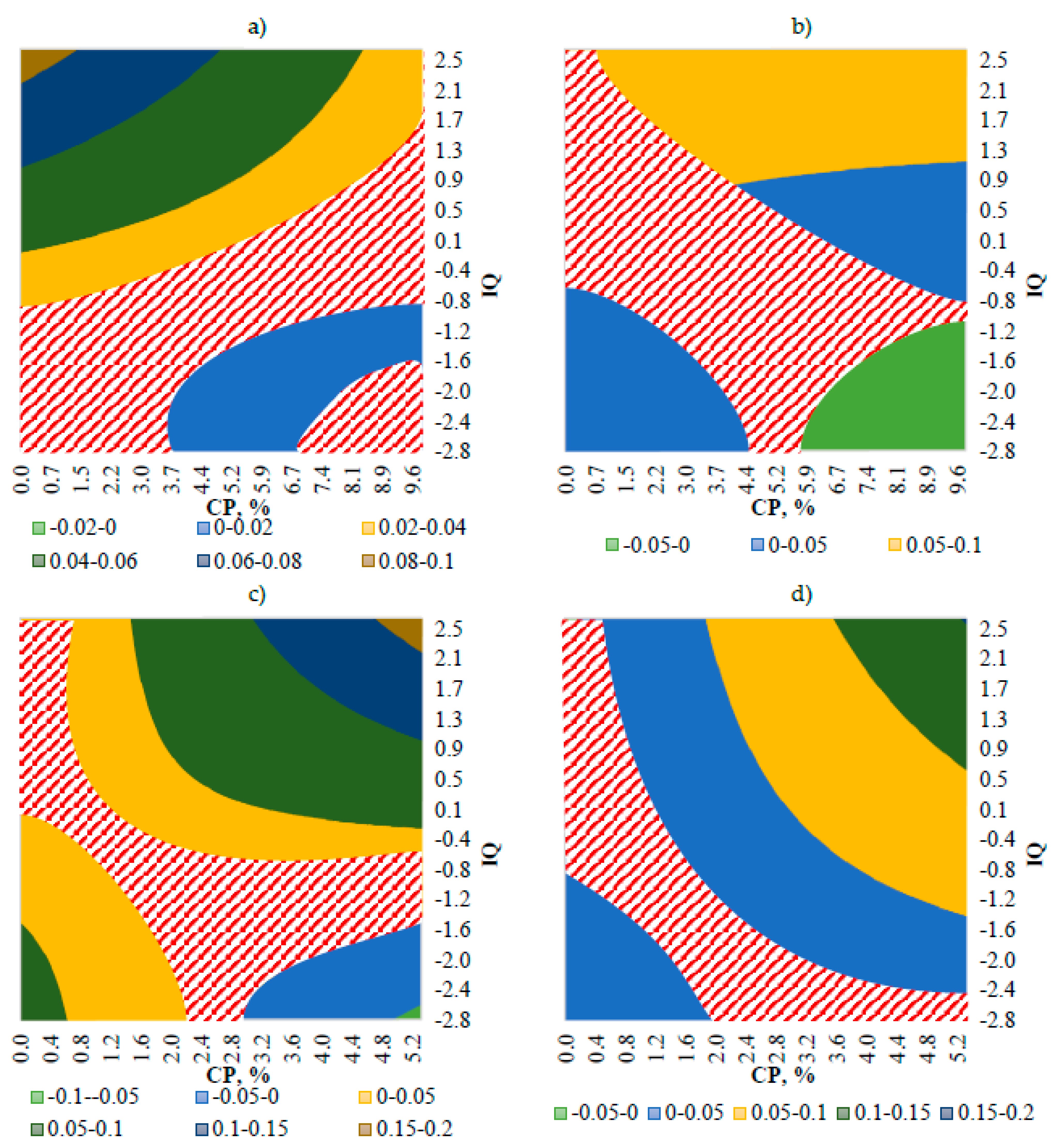
4.2. Non-Linear Effects of CP on Growth Moderated by Institutional Quality

Estimated statistically significant positive coefficients on $CP$ and negative coefficients on its squared term, i.e., $C{P}^2$, suggest that the relationship between the intensity of CP commitments and growth (in terms of per capita GDP and productivity) is in the form of an inverted U-shaped letter. This means that even though the impact of CP on growth is positive, its marginal effect is diminishing, and there is a level of intensity of the CP commitments above which its marginal effect becomes negative. Our estimates show5 that over the 2000–2006 programming period, the turning point is about 0.45–0.54 percent considering per capita GDP, and 0.65–0.73 percent considering productivity. Over the 2007–2013 programming period, the turning points are 0.80–0.85 and 1.03–1.05 percent, respectively. Slightly higher turning points over the 2000–2007 programming period suggest that a more significant proportion of the commitments had a positive effect on growth, which confirms previous contributions, which highlight that CP was more successful over 2007–2013 compared to 2000–2006.

Comparing the effects of CP on growth in terms of per capita GDP and productivity at different disaggregation levels, it becomes clear that they are very diverse. CP had a much more significant positive impact at the NUTS2 disaggregation level compared to the NUTS3, and on economic growth compared to productivity growth. Even though differences in the effect over the 2007–2013 programming period became smaller, they remained huge. The impact of CP at the NUTS2 level is bigger by about 1.6–1.9 times (compared to 2.6–4.3 over 2000–2006), and the effect on per capita GDP growth is bigger by roughly 1.1–1.3 times (compared to 1.2–2.0 over 2000–2006). Differences in the impact over the 2007–2013 programming period became smaller mainly due to the decreased effect of CP at the NUTS2 disaggregation level. The impact on productivity and economic growth fell by 1.4–1.5 times compared to 2000–2006.

Estimated statistically significant and positive coefficients on the multiplicative term $CP·IQ$ suggest that institutional quality positively moderates the effect of CP on growth. In other words, we might expect more positive outcomes of CP if it is implemented in regions with a more favourable institutional environment. Moreover, estimations suggest that institutions are more critical in transforming CP commitments to productivity growth compared to per capita GDP growth, and that this importance increased even more during the economic downturn. If we assume that the relationship between CP and growth is linear6, the increase of the IQ from 0 to 1 would enhance the effect of CP7 on growth over the 2000–2006 programming period from 1.00–2.57 to 2.10–3.58 percent considering per capita GDP and from 0.51–2.16 to 1.74–3.45 percent considering productivity. Over the 2007–2013 programming period, the effect would increase from 1.05–1.68 to 1.89–2.63 and from 0.84–1.59 to 2.32–3.02 percent, respectively. Therefore, estimations suggest that institutions are vital in boosting growth and its effect is roughly the same considering per capita GDP and productivity. Moreover, the importance of institutions became bigger over the economic downturn, especially at the NUTS3 level.

Estimated statistically significant coefficients on multiplicative term $C{P}^2·IQ$ show that institutional quality moderates not only the linear relationship between the CP and growth8 but also the marginal effect of the CP. Moreover, positive coefficients show that the more favourable institutional environment, the higher the tipping point above which the marginal impact of CP on growth becomes negligible. For example, other factors being equal, the increase of the IQ from 0 up to 1 would increase the turning point over the 2000–2006 programming period from 0.45–0.54 to 0.77–1.98 percent, considering per capita GDP, and from 0.65–0.73 to 1.29–1.34 percent, considering productivity9. Over the 2007–2013 programming period, the turning points would increase from 0.80–0.85 to 1.50–2.62 and from 1.02–1.04 to 1.45–1.8 percent, respectively. If we account for all interactions, the increase of the IQ from 0 up to 1 would increase the turning point over the 2000–2006 programming period up to 1.62–2.75 percent, considering per capita GDP, and up to 2.05–4.58 percent, considering productivity. Over the 2007–2013 programming period, the turning points would increase up to 2.35–4.73 and up to 2.74–5.04 percent, respectively.

By the logic of our proposed model, the estimated marginal effect of CP on growth is conditional, i.e., it is moderated by the institutional quality and the intensity of the CP commitments. Therefore, the estimated slope coefficients of growth on CP and their standard errors are conditional as well. Figure 1 and Figure 2 show the estimated marginal effects of CP on growth over the observed range of values for institutional quality and CP over both programming periods under consideration. Based on calculations using Equation (5), Figure 1 and Figure 2 show which combinations of IQ and CP values yield statistically significant and insignificant slope coefficients, which are estimated based on the first set of brackets in Equation (3).

Figure 1 and Figure 2, irrespective of the disaggregation level and dependent variable under consideration, show a similar finding: CP has a positive effect on per capita GDP and productivity growth. However, CP commitments are subject to diminishing effects, especially in regions with a low level of institutional quality. A higher level of CP commitments’ intensities in regions with an unfavourable institutional environment (going from the bottom left corner to the bottom right corner in the figures) is related to a decrease in the positive marginal effect and, subsequently, an increase in the negative marginal effect. The institutional quality changes the form of the relationship between CP and growth. Going from the bottom right corner to the top right corner in the figures, the institutional environment changes from unfavourable to favourable and the marginal effect of the same level of the CP commitments’ intensities changes from negative to positive. Comparing the 2000–2006 and 2007–2013 programming periods, it is clear that, over the latter, much more combinations of values for CP and institutional quality yield a statistically significant effect on growth. What is more important is that more combinations yield a positive effect, and that this is due to higher levels of institutional environments over 2007–2013 compared to 2000–2006.

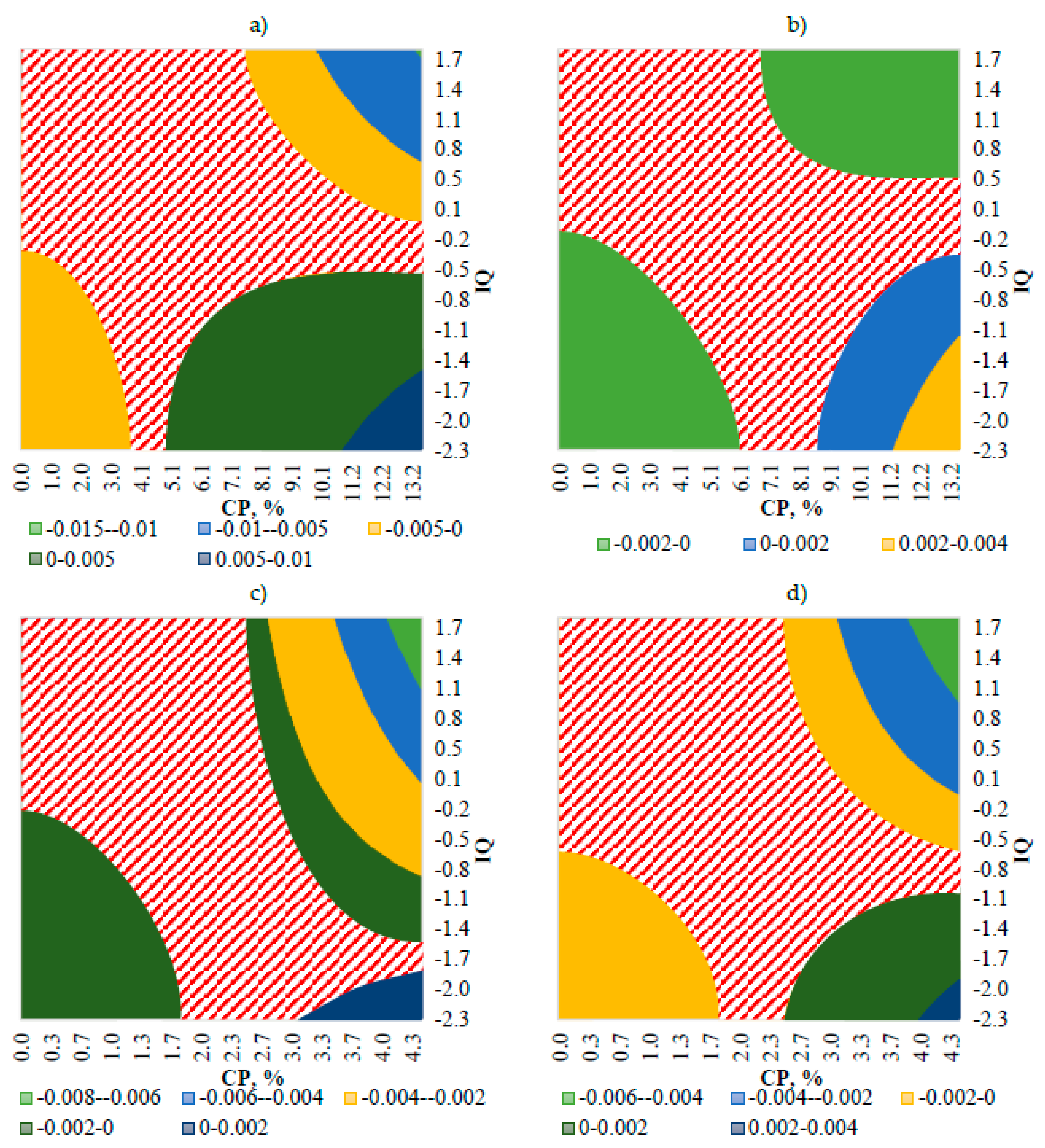
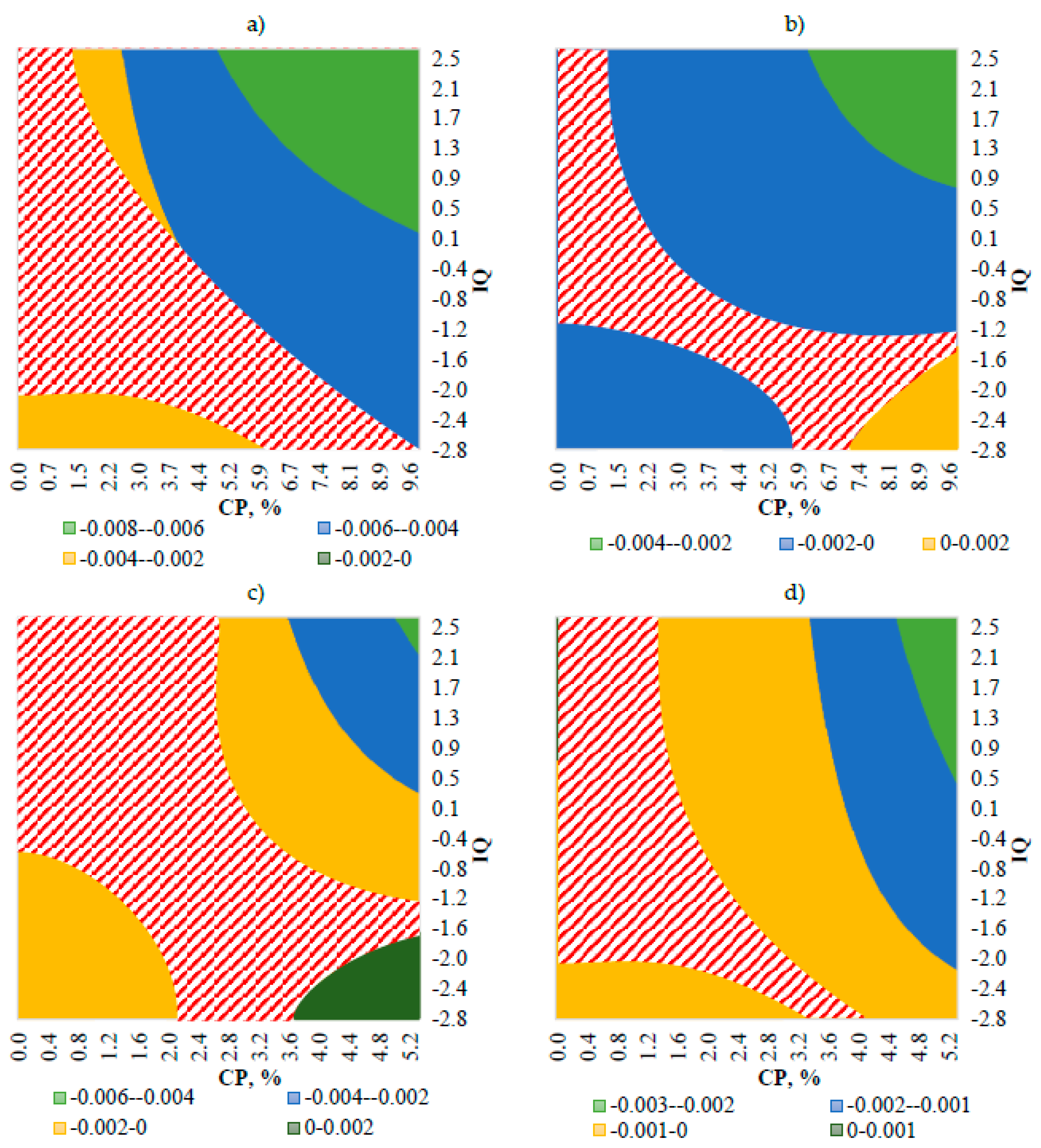
4.3. Non-Linear Convergence Outcomes of CP Moderated by the Institutional Quality

The estimated coefficients on $ln\left(Y\right)$ are statistically significant and negative, indicating that conditional β-convergence was present over both programming periods. Convergence was faster10 by 1.30–1.73 times in terms of productivity compared to per capita GDP over the 2000–2006 programming period, i.e., when the economy was booming, but then slowed down by 2.62–2.88 times when the economy was declining. On the contrary, the speed of convergence, in terms of per capita GDP, increased by 1.42–1.43 times over the 2007–2013 period. This could have been caused by higher economic decline in most developed regions, due to the financial crisis, compared to the least developed areas in which economies were heavily revived using CP funding. The estimated rate of convergence was similar at the NUTS2 and 3 disaggregation levels.

The negative coefficient on interaction $ln\left(Y\right)·CP$ suggests that CP speeds up the convergence process, i.e., regions with higher intensities of CP commitments experienced faster convergence. If we compare two regions, both with the level of institutional quality equal to zero, the one that has an intensity of CP commitments equal to 1 will experience convergence faster by 1.14–1.28 times in terms of per capita GDP, and by 1.08–1.22 times in terms of productivity over the 2000–2006 programming period, and faster by 1.12–1.13 and by 1.28–1.30 times over the 2007–2013 programming period, respectively, compared to another without any CP funding. Over the 2000–2006 programming period, CP had a twice bigger effect on the convergence between NUTS2 regions compared to NUTS3 regions. Estimations suggest that the importance of CP for convergence increased at the NUTS3 level and decreased at the NUTS2 level over the 2007–2013 period, when regions faced the consequences of the financial crisis.

The statistically significant and negative coefficient on the multiplicative term $ln\left(Y\right)·IQ$ suggests that if we already control the initial development level, we can expect faster convergence in regions where the institutional environment is more favourable. It means that where there are two regions with the same level of initial development, we might expect faster growth and thus convergence in the one with a higher level of institutional quality. Even more, the effect of institutions is slightly larger on regional convergence at the NUTS3 disaggregation level and over the 2007–2013 programming period. If we compare two regions11, both with an intensity of CP commitments equal to zero, the one that has a level of institutional quality equal to 1 will experience convergence faster by 1.50–1.68 times in terms of per capita GDP, and by 1.37–1.41 times in terms of productivity over the 2000–2006 programming period, and faster by 1.39–1.50 and by 2.10–2.08 times over the 2007–2013 programming period, respectively, compared to another with a level of institutional quality equal to 0.

The statistically significant and negative estimated coefficient on the multiplicative term $ln\left(Y\right)·CP·IQ$ suggests that after controlling the initial level of regional development and the effects of CP and institutional quality on convergence separately, CP in a favourable institutional environment can additionally burst regional convergence. This means that CP commitments and a favourable institutional environment combined will probably lead to faster convergence than just good institutions or only CP funding.

Estimated statistically significant and positive coefficients on the multiplicative term $ln\left(Y\right)·C{P}^2$ show that the marginal effect of CP on convergence is diminishing, i.e., additional CP commitments have a diminishing marginal impact on boosting convergence. The estimated turning point12 when additional CP commitments no longer accelerate convergence is at about 1.0–1.3 percent over the 2000–2006 programming period, and at about 1.9–2.3 over the 2007–2013 programming period. Higher turning points over the 2007–2013 programming period suggest that a more significant proportion of commitments had a positive effect on convergence, which confirms the findings of previous contributions, which highlight that CP was more successful over the 2007–2013 programming period compared to 2000–2006.

The estimated statistically significant coefficients on the multiplicative term $ln\left(Y\right)·C{P}^2·IQ$ indicate that the institutional environment is affecting the marginal effect of CP on convergence. Moreover, coefficients being negative means that a more favourable institutional environment shifts the tipping point to the right, reducing the probability of negative marginal effects in more intensively funded regions.

By the logic of our proposed model, the estimated correlation between $ln\left(Y\right)$ and growth, i.e., convergence, is conditional, since it is non-linearly related to the intensity of the CP commitments, and institutional quality moderates this relation. Therefore, the estimated slope coefficients of growth on $ln\left(Y\right)$ (β-convergence coefficients) and their standard errors are conditional as well. Figure 3 and Figure 4 show the estimated slope coefficients of growth on $ln\left(Y\right)$ over the observed range of values for institutional quality and CP for both programming periods under consideration. Based on calculations using Equation (7), Figure 3 and Figure 4 show which combinations of IQ and CP values yield statistically significant and insignificant slope coefficients, estimated based on the second set of brackets in Equation (3).

Figure 3 and Figure 4 show that the speed of convergence is affected by CP and institutional quality. Increasing intensity of the CP commitments leads to a diminishing marginal effect of CP on convergence, and this is the case for both disaggregation levels, for both dependent variables, and over both programming periods under consideration. In regions with an unfavourable institutional environment, the exceptionally high intensity of the CP commitments leads to a negative marginal effect of CP on convergence, which increases when intensity is higher. Institutional quality shapes the non-linear effect of CP on convergence, i.e., in a favourable institutional environment, there is almost no sign of diminishing marginal effects. On the contrary, some estimations suggest that in regions with the most favourable environments, CP has an increasing marginal impact on convergence, i.e., a relatively high intensity of CP commitments still leads to a positive marginal impact on convergence, which increases. We also see that over the 2007–2013 programming period much more combinations of CP intensity and institution quality ensured a statistically significant effect on convergence compared to the 2000–2006 programming period. Just in rear cases, when the intensity of CP commitments was exceptionally high and institutional quality was exceptionally low, the estimated slope coefficient was positive, i.e., signalling a negative marginal effect on convergence.

Despite the fact that the majority of research, including ours, reveals the positive impact of CP on economic growth and/or convergence, there are still discussions that contend that it does not succeed the intended objectives. Empirical evidence shows the heterogeneous distribution of CP’s regional impact across the EU. It suggests that the institutional quality of individual regions has a significant role in the success (or failure) of its implementation. There is a consensus that post-2020, CP must be reformed to respond to new demands and challenges. The uneven development of the Member States and their institutional environments lead to different constraints on the impact of CP. Less developed regions in the EU have a higher demand for CP funding to support structural reforms. Still, they have limited resources, including limited institutional capabilities, which might hinder the proper implementation of the CP. On the other hand, more developed regions are discouraged from implementing structural reforms domestically to receive CP funding for these reforms.

5. Conclusions

We supplemented the existing literature on the impact of CP in a few ways: (i) by proposing to extend the conventional β-convergence model by augmenting it with 2- and 3-way multiplicative terms to examine how institutional quality moderates the non-linear impact of CP on growth and convergence; (ii) by proposing and computing conditional marginal effects and their standard errors, we show that the effect of CP on growth and convergence is largely heterogeneous across the EU in terms of its direction and significance.

Our estimations are in line with previous research showing that the marginal effect of CP and the amount of CP investments correlate negatively. However, our findings show that institutional quality is able to change this correlation, and imply that improvements in the institutional environment are fundamental for CP to boost economic growth and convergence in a more significant number of regions. Our results confirm the impact heterogeneity of CP across the EU. We find the levels of institutional quality and CP intensity for which the estimated marginal growth and convergence effect of CP is positive, and the levels for which this effect is negative. The same is considered for the statistical significance of CP’s impact. We show that there is no one single tipping point above which CP has no additional positive effect. On the contrary, our study confirms many tipping points which depend on the institutional environment, pointing out the need for the relocation of funds in favour of improving regional institutional quality, which could lead to faster economic growth and convergence with fewer funds.

Our research confirms the findings of previous contributions, which highlight that CP was more successful over the 2007–2013 programming period compared to the 2000–2006 period, as more considerable attention was devoted to performance management (using means of evaluation, monitoring, performance and expenditure reserves) to increase the effectiveness of managing the EU structural funds, making management more integrated into national economic and financial systems.

The policy implications from this research point towards the need for enhanced administrative capacity in lagging EU regions, not only focusing on fundamental economic problems but also on implementing comprehensive and appropriate regional policies through the adoption of managerial innovations and the accumulation of human capital for improving institutional environments. Summarising the results of our research and the insights of previous contributions, three main streams of policy can be distinguished: (i) voiding CP funding to the recipient regions where CP has no impact on economic growth or convergence; (ii) reallocating funding from regions where they do not achieve the intended objectives to the regions where the impact is positive; (iii) changing the denomination of CP funding, as the heterogeneous impact of CP is determined with an institutional absorptive capacity. Moreover, less autonomy in the distribution of the CP funds must be given to the Member States and their regions with low institutional quality. This recommendation is in line with Charron’s (2016) findings that if regions with low institutional quality have low autonomy, the risk of failing to achieve the absorption of funds, as well as to achieve the goals of CP, is reduced, and vice versa.

Our research confirms the importance of the localised institutional environment on the moderating impact of CP. Improving Member States’ administrative capacity at a regional level should become a new priority for CP. Since empirical findings suggest that regional policy models and economic impacts are highly heterogeneous across countries, a nation-based regional policy implementing overarching objectives of each Member State could complement the existing place-based approach. Greater adaptability at national and regional levels could be the best response to the renationalisation of CP.

Previous studies show different results of national intervention models—while some are effective, others are not. Suppose that the results do not achieve the intended objectives. In that case, Member States should take full responsibility and be empowered to act accordingly, perhaps not granting the right for funding distribution to the local authorities and ensuring the equal distribution of funds among small territorial units. Little impact in the least developed regions often reflects inadequate national-level strategic policies. The heterogeneity of the CP impact at the regional level suggests that Member States could be given more freedom to choose how to invest CP funds in exchange for greater accountability, more transparent evidence-based strategic decisions, robust evaluation procedures, and improved institutional quality.

The main limitation of our research is related to the lack of data to proxy institutional environments at the NUTS3 level using EQI. As discussed in the paper, we used NUTS2 data to proxy institution quality across all NUTS3 regions within NUTS2 regions. Even though we addressed the problem of this strategy to create clusters from the statistical point of view by using cluster robust standard errors, our strategy ignores the possible heterogeneity of institutional environments within NUTS2 regions. The temporary solution for this limitation is to look for alternative variables available at the NUTS3 level to serve as proxies for the institutional environment. The permanent solution would be the collection of data necessary to estimate EQI on a yearly basis at the NUTS3 level, since we find more and more evidence that local institutions play a crucial role in mediating the effectiveness of EU-wide place-based policies aiming to boost growth and convergence. Thus, having a robust indicator of institutional quality at a low disaggregation level would allow us to monitor dynamics and tackle the necessary problems before directing CP funding.

References

1. Arbolino, Roberta, and Raffaele Boffardi. 2017. The Impact of Institutional Quality and Efficient Cohesion Investments on Economic Growth Evidence from Italian Regions. Sustainability 9: 1432. [Google Scholar] [CrossRef] [Green Version]
2. Arbolino, Roberta, Paolo Di Caro, and Ugo Marani. 2020. Did the governance of EU funds help Italian regional labour markets during the Great Recession? Journal Common Market Studies 58: 235–55. [Google Scholar] [CrossRef]
3. Bähr, Cornelius. 2008. How does Sub-National Autonomy Affect the Effectiveness of Structural Funds? Kyklos 61: 3–18. [Google Scholar] [CrossRef]
4. Barca, F. 2009. An Agenda for a Reformed Cohesion Policy: A Place-based Approach to Meeting European Union Challenges and Expectations. Available online: http://www.europarl.europa.eu/meetdocs/2009_2014/documents/regi/dv/barca_report_/barca_report_en.pdf (accessed on 27 September 2019).
5. Becker, Sascha O., Peter H. Egger, and Maximilian Von Ehrlich. 2012. Too Much of a Good Thing? On the Growth Effects of the EU’s Regional Policy. European Economic Review 56: 648–68. [Google Scholar] [CrossRef] [Green Version]
6. Becker, Sascha O., Peter H. Egger, and Maximilian Von Ehrlich. 2013. Absorptive capacity and the growth and investment effects of regional transfers: A regression discontinuity design with heterogeneous treatment effects. American Economic Journal 5: 29–77. [Google Scholar] [CrossRef] [Green Version]
7. Becker, Sascha O., Peter H. Egger, and Maximilian Von Ehrlich. 2015. Regional Policy (Chapter 17). In Handbook of the Economics of European Integration. Edited by H. Badinger and V. Nitsch. London: Routledge. [Google Scholar]
8. Becker, Sascha O., Peter H. Egger, and Maximilian Von Ehrlich. 2018. Effects of EU Regional Policy: 1989–2013. Regional Science and Urban Economics 69: 143–52. [Google Scholar] [CrossRef]
9. Beugelsdijk, Maaike, and Sylvester C. W. Eijffinger. 2005. The effectiveness of structural policy in the European Union: An empirical analysis for the EU–15 in 1995–2001. Journal of Common Market Studies 43: 37–51. [Google Scholar] [CrossRef] [Green Version]
10. Bourdin, Sebastien. 2019. Does the Cohesion Policy Have the Same Influence on Growth Everywhere? A Geographically Weighted Regression Approach in Central and Eastern Europe. Economic Geography 95: 256–87. [Google Scholar] [CrossRef]
11. Brambor, Thomas, William Roberts Clark, and Matt Golder. 2006. Understanding Interaction Models: Improving Empirical Analyses. Political Analysis 14: 63–82. [Google Scholar] [CrossRef] [Green Version]
12. Butkus, Mindaugas, Alma Mačiulytė-Šniukienė, and Kristina Matuzevičiūtė. 2020a. The role of institutions in shaping geography of development disparities across European Union. Geografický Časopis 72: 25–47. [Google Scholar] [CrossRef]
13. Butkus, Mindaugas, Diana Cibulskienė, Alma Mačiulytė-Šniukienė, and Kristina Matuzevičiutė. 2020b. Non-linear and Lagging Convergence Effects of the EU’s Regional Support at NUTS3 Level. Journal of Urban and Regional Analysis 12: 35–52. [Google Scholar] [CrossRef]
14. Butkus, Mindaugas, Diana Cibulskienė, Alma Mačiulytė-Šniukienė, and Kristina Matuzevičiutė. 2020c. Mediating Effects of Cohesion Policy and Institutional Quality on Convergence between EU Regions: An Examination Based on a Conditional Β-convergence Model with a 3-Way Multiplicative Term. Sustainability 12: 3025. [Google Scholar] [CrossRef] [Green Version]
15. Butkus, Mindaugas, Diana Cibulskienė, Alma Mačiulytė-Šniukienė, and Kristina Matuzevičiutė. 2020d. Does Financial Support from ERDF and CF Contribute to Convergence in the EU? Empirical Evidence at NUTS3 Level. Prague Economic Papers 29: 315–29. [Google Scholar] [CrossRef]
16. Casula, Mattia. 2020. Under which conditions is Cohesion Policy effective: Proposing an Hirschmanian approach to EU structural funds. Regional and Federal Studies, 1–27. [Google Scholar] [CrossRef]
17. Cerqua, Augusto, and Guido Pellegrini. 2018. Are we spending too much to grow? The case of Structural Funds. Journal of Regional Science 58: 535–63. [Google Scholar] [CrossRef]
18. Charron, Nicholas. 2016. Explaining the allocation of regional Structural Funds: The conditional effect of governance and self-rule. European Union Politics 17: 1–22. [Google Scholar] [CrossRef]
19. Charron, Nicholas, Victor Lapuente, and Bo Rothstein, eds. 2010. Measuring the Quality of Government and Subnational Variation. Report for the European Commission Directorate–General Regional Policy, Directorate Regional Policy. Gothenburg: Quality of Quality of Government and Returns of Investment: Cohesion Expenditure in European Regions 1289 Government Institute, Department of Political Science, University of Gothenburg, Available online: http://ec.europa.eu/regional_policy/sources/docgener/studies/pdf/2010_government_1.pdf (accessed on 27 June 2019).
20. Charron, Nicholas, Lewis Dijkstra, and Victor Lapuente. 2014. Regional governance matters: Quality of government within European Union member states. Regional Studies 48: 68–90. [Google Scholar] [CrossRef]
21. Ciffolilli, Andrea, Stefano Condello, Marco Pompili, and Roman Roemish. 2015. Geography of Expenditure. Final Report. Work Package 13. Ex post evaluation of Cohesion Policy Programmes 2007–2013, Focusing on the European Regional Development Fund (ERDF) and the Cohesion Fund (CF). Available online: https://ec.europa.eu/regional_policy/sources/docgener/evaluation/pdf/expost2013/wp13_final_report_en.pdf (accessed on 27 June 2019).
22. Crescenzi, Riccardo, and Mara Giua. 2014. The EU Cohesion Policy in Context: Regional Growth and the Influence of Agricultural and Rural Development Policies. LSE’ Europe in Question. Discussion Paper Series Paper, 85. Available online: http://aei.pitt.edu/93663/ (accessed on 26 April 2020).
23. Crescenzi, Riccardo, and Mara Giua. 2020. One or many Cohesion Policies of the European Union? On the differential economic impacts of Cohesion Policy across member states. Regional Studies 54: 10–20. [Google Scholar] [CrossRef] [Green Version]
24. Dall’erba, Sandy, Rachel Guillain, and Julie Le Gallo. 2009. Impact of structural funds on regional growth: How to reconsider a 9-year-old black box. Région et Développement 30: 77–100. [Google Scholar]
25. Del Bo, Chiara, Massimo Florio, Emanuela Sirtori, and Silvia Vignetti. 2011. Additionality and Regional Development: Are EU Structural Funds Complements or Substitutes of National Public Finance? CSIL Working Paper N. 01/2011. Milan: CSIL. [Google Scholar]
26. Dellmuth, Lisa Maria, Dominik Schraff, and Michael F. Stoffel. 2017. Distributive Politics, Electoral Institutions and European Structural and Investment Funding: Evidence from Italy and France. Journal of Common Market Studies 55: 275–93. [Google Scholar] [CrossRef] [Green Version]
27. Di Cataldo, Marco. 2017. The impact of EU Objective 1 funds on regional development: Evidence from the UK and the prospect of Brexit. Journal of Regional Science 57: 814–39. [Google Scholar] [CrossRef]
28. Di Cataldo, Marco, and Vassilis Monastiriotis. 2018. An Assessment of EU Cohesion Policy in the UK Regions: Direct Effects and the Dividend of Targeting. LEQS Paper 135. Available online: https://ssrn.com/abstract=3198691 (accessed on 17 June 2019).
29. Di Cataldo, Marco, and Vassilis Monastiriotis. 2020. Regional needs, regional targeting and regional growth: An assessment of EU Cohesion Policy in UK regions. Regional Studies 54: 35–47. [Google Scholar] [CrossRef] [Green Version]
30. Eberle, Jonathan, and Thomas Brenner. 2016. More Bucks, More Growth, More Justice? The Effects of Regional Structural Funds on Regional Economic Growth and Convergence in Germany. Working Papers on Innovation and Space, 01.16. Marburg: Philipps University Marburg, Department of Geography, Available online: http://hdl.handle.net/10419/147971 (accessed on 17 June 2019).
31. Ederveen, Sjef, Henri L.F. De Groot, and Richard Nahuis. 2006. Fertile soil for structural funds? A panel data analysis of the conditional effectiveness of European cohesion policy. Kyklos 59: 17–42. [Google Scholar] [CrossRef]
32. Esposti, Roberto, and Stefania Bussoletti. 2008. Impact of objective 1 funds on regional growth convergence in the European Union: A panel–data approach. Regional Studies 42: 159–73. [Google Scholar] [CrossRef]
33. European Commission. 2016. Measuring the impact of Structural and Cohesion Funds Using Regression Discontinuity Design in EU27 in the period 1994–2011, Ex Post Evaluation of Cohesion Policy Programmes 2007–2013, focusing on the European Regional Development Fund (ERDF) and the Cohesion Fund (CF). Final Technical Report, Work Package 14c—Tasks 2 and 3. Available online: https://ec.europa.eu/regional_policy/sources/docgener/evaluation/pdf/expost2013/wp14c_task1_final_report_en.pdf (accessed on 1 June 2019).
34. European Commission. 2019. European Structural and Investment Funds. Available online: https://cohesiondata.ec.europa.eu/overview (accessed on 26 April 2020).
35. Florio, Massimo, and Luigi Moretti. 2014. The Effect of Business Support on Employment in Manufacturing: Evidence from the European Union Structural Funds in Germany, Italy and Spain. European Planning Studies 22: 1802–23. [Google Scholar] [CrossRef]
36. Fratesi, Ugo, and Giovanni Perucca. 2014. Territorial Capital and the Effectiveness of Cohesion Policies: An Assessment for CEE Regions, GRINCOH. Working Paper Series, 8.05. Available online: http://www.grincoh.eu/media/serie_8__cohesion_and_its_dimensions/grincoh_wp8.05_fratesi_perucca.pdf (accessed on 1 June 2019).
37. Gagliardi, Luisa, and Marco Percoco. 2017. The impact of European Cohesion Policy in urban and rural regions. Regional Studies 51: 857–68. [Google Scholar] [CrossRef]
38. Ganau, Roberto, and Andrés Rodríguez-Pose. 2019. Do high-quality local institutions shape labour productivity in Western European manufacturing firms? Papers in Regional Science 98: 1633–66. [Google Scholar] [CrossRef]
39. Gorzelak, Grzegorz. 2016. Cohesion Policy and regional development. In 33EU Cohesion Policy—Reassessing Performance and Direction. Edited by J. Bachtler, P. Berkowitz, S. Hardy and T. Muravska. London: Routledge. [Google Scholar] [CrossRef]
40. Host, Alen, Vinko Zaninović, and Krešimir Parat. 2017. Cohesion Policy Instruments and Economic Growth: Do Institutions Matter? Ekonomiska Misao I Praksa 2: 541–59. [Google Scholar]
41. Kyriacou, Andreas P., and Oriol Roca-Sagalés. 2012. The Impact of EU Structural Funds on Regional Disparities within Member States. Environment and Planning C: Politics and Space 30: 267–81. [Google Scholar] [CrossRef] [Green Version]
42. Leona, S. Aiken, and Stephen G. West. 1991. Multiple Regression: Testing and Interpreting Interactions. London: Sage. [Google Scholar]
43. Lippman, S. S., and John J. McCall. 2015. Three Principal–Agent Models with Asymmetric Information. In International Encyclopedia of the Social & Behavioral Sciences, 2nd ed. Edited by J. D. Wright. Oxford: Elsevier Ltd. [Google Scholar]
44. Marzinotto, Benedicta. 2012. The Growth Effects of EU Cohesion Policy: A Meta–Analysis. Bruegel Working Paper No. 2012/14. Available online: https://www.econstor.eu/bitstream/10419/78011/1/728570688.pdf (accessed on 10 June 2020).
45. Maynou, Laia, Marc Saez, Andreas Kyriacou, and Jordi Bacaria. 2016. The Impact of Structural and Cohesion Funds on Eurozone Convergence, 1990–2010. Regional Studies 50: 1127–39. [Google Scholar] [CrossRef]
46. Olson, Mancur. 1965. The Logic of Collective Action: Public Goods and the Theory of Groups. Cambridge and London: Harvard University Press. [Google Scholar]
47. Pellegrini, Guido, and Augusto Cerqua. 2016. Measuring the impact of intensity of treatment using RDD and covariates: The case of Structural Funds. Paper presented at 57th RSA Annual Conference, Milano, Italy, October 20–22. [Google Scholar]
48. Pellegrini, Guido, Federica Busillo, Teo Muccigrosso, Ornella Tarola, and Flavia Terribile. 2013. Measuring the Impact of the European Regional Policy on Economic Growth: A Regression Discontinuity Design Approach. Papers in Regional Science 92: 217–33. [Google Scholar] [CrossRef]
49. Piętak, Łukasz. 2018. Did Structural Funds Affect Economic Growth and Convergence across Regions? Spanish Case in the Years 1989–2016. INE PAN Working Paper Series, No. 44. Available online: http://inepan.pl/wp–content/uploads/2016/07/working–papers–44–Hiszpania–Pietak.pdf (accessed on 10 June 2020).
50. Pinho, Carlos, Celeste Varum, and Micaela Antunes. 2015a. Structural Funds and European Regional Growth: Comparison of Effects among Different Programming Periods. European Planning Studies 23: 1302–26. [Google Scholar] [CrossRef] [Green Version]
51. Pinho, Carlos, Celeste Varum, and Micaela Antunes. 2015b. Under What Conditions Do Structural Funds Play a Significant Role in European Regional Economic Growth? Some Evidence from Recent Panel Data. Journal of Economic Issues 49: 749–71. [Google Scholar] [CrossRef] [Green Version]
52. Pontarollo, Nicola. 2017. Does Cohesion Policy affect regional growth? New evidence from a semi-parametric approach. In EU Cohesion Policy. Edited by J. Bachtler, P. Berkowitz, S. Hardy and T. Muravska. London and New York: Routledge, pp. 93–108. [Google Scholar]
53. Rodríguez-Pose, Andrés, and Ugo Fratesi. 2004. Between Development and Social Policies: The Impact of European Structural Funds in Objective 1 Regions. Regional Studies 38: 97–113. [Google Scholar] [CrossRef]
54. Rodríguez-Pose, Andrés, and Katja Novak. 2013. Learning processes and economic returns in European Cohesion Policy. Investigaciones Regionales 25: 7–26. [Google Scholar]
55. Rodríguez-Pose, Andrés, and Enrique Garcilazo. 2015. Quality of Government and the Returns of Investment: Examining the Impact of Cohesion Expenditure in European Regions. Regional Studies 49: 1274–90. [Google Scholar] [CrossRef]
56. Rodríguez-Pose, Andrés, and Tobias Ketterer. 2019. Institutional change and the development of lagging regions in Europe. Regional Studies 54: 974–86. [Google Scholar] [CrossRef] [Green Version]
57. SWECO. 2008. Final Report—ERDF and CF Regional Expenditure Contract No. 2007.CE.16.0.AT.036. Available online: https://ec.europa.eu/regional_policy/sources/docgener/evaluation/pdf/expost2006/expenditure_final.pdf (accessed on 17 July 2020).
58. Szitásiová, Valeria, Monika Martišková, and Miroslav Šipikal. 2014. Substitution Effect of Public Support Programs at Local Level. Transylvanian Review of Administrative Sciences 10: 167–82. [Google Scholar]
59. Wostner, Peter, and Sonja Šlander. 2009. The Effectiveness of EU Cohesion Policy Revisited: Are eu Funds Really Additional? European Policy Research Paper 69: 1–26. Available online: https://strathprints.strath.ac.uk/70313/1/EPRP_69.pdf (accessed on 17 July 2020).
Figure 1. The estimated conditional marginal effect of CP on growth (the slope coefficient) moderated by the institutional quality and the intensity of the CP commitments, i.e., γ ^ 1 + γ ^ 2 · C P i , t + b ^ 2 · I Q i , t + b ^ 6 · C P i , t · I Q i , t , over the 2000–2006 programming period. The white area with red stripes represents combinations of institutional quality and the intensity of the CP commitments for which the estimated slope coefficient is statistically insignificant. Areas in colour represent combinations of institutional quality and the intensity of the CP commitments for which the estimated marginal effect of CP on growth (in percentages) is statistically significant. (a) Marginal effect on per capita GDP growth at the NUTS3 disaggregation level. (b) Marginal effect on productivity growth at the NUTS3 disaggregation level. (c) Marginal effect on per capita GDP growth at the NUTS2 disaggregation level. (d) Marginal effect on productivity growth at the NUTS2 disaggregation level.
Economies 09 00103 g001
Figure 2. The estimated conditional marginal effect of CP on growth (the slope coefficient) moderated by the institutional quality and the intensity of the CP commitments, i.e., γ ^ 1 + γ ^ 2 · C P i , t + b ^ 2 · I Q i , t + b ^ 6 · C P i , t · I Q i , t , over the 2007–2013 programming period. The white area with red stripes represents combinations of institutional quality and the intensity of the CP commitments for which the estimated slope coefficient is statistically insignificant. Areas in colour represent combinations of institutional quality and the intensity of the CP commitments for which the estimated marginal effect of CP on growth (in percentages) is statistically significant. (a) Marginal effect on per capita GDP growth at the NUTS3 disaggregation level. (b) Marginal effect on productivity growth at the NUTS3 disaggregation level. (c) Marginal effect on per capita GDP growth at the NUTS2 disaggregation level. (d) Marginal effect on productivity growth at the NUTS2 disaggregation level.
Economies 09 00103 g002
Figure 3. The estimated conditional correlation between l n ( Y ) and growth (the slope coefficient of growth on l n ( Y ) , i.e., the coefficient of conditional β-convergence) moderated by the institutional quality and the intensity of the CP commitments, i.e., β ^ + b ^ 1 · C P i , t + b ^ 3 · I Q i , t + b ^ 4 · I Q i , t · C P i , t + b ^ 5 · C P i , t 2 + b ^ 7 · I Q i , t · C P i , t 2 , over the 2000–2006 programming period. The white area with red stripes represents combinations of institutional quality and the intensity of the CP commitments for which the estimated slope coefficient is statistically insignificant. Areas in colour represent combinations of institutional quality and the intensity of the CP commitments for which the estimated conditional β-convergence coefficient is statistically significant. (a) The slope coefficient of per capita GDP growth on l n ( Y ) at the NUTS3 disaggregation level. (b) The slope coefficient of productivity growth on l n ( Y ) at the NUTS3 disaggregation level. (c) The slope coefficient of per capita GDP growth on l n ( Y ) at the NUTS2 disaggregation level. (d) The slope coefficient of productivity growth on l n ( Y ) at the NUTS2 disaggregation level.
Economies 09 00103 g003
Figure 4. The estimated conditional correlation between l n ( Y ) and growth (the slope coefficient of growth on l n ( Y ) , i.e., the coefficient of conditional β-convergence) moderated by the institutional quality and the intensity of the CP commitments, i.e., β ^ + b ^ 1 · C P i , t + b ^ 3 · I Q i , t + b ^ 4 · I Q i , t · C P i , t + b ^ 5 · C P i , t 2 + b ^ 7 · I Q i , t · C P i , t 2 , over the 2007–2013 programming period. The white area with red stripes represents combinations of institutional quality and the intensity of the CP commitments for which the estimated slope coefficient is statistically insignificant. Areas in colour represent combinations of institutional quality and the intensity of the CP commitments for which the estimated conditional β-convergence coefficient is statistically significant. (a) The slope coefficient of per capita GDP growth on l n ( Y ) at the NUTS3 disaggregation level. (b) The slope coefficient of productivity growth on l n ( Y ) at the NUTS3 disaggregation level. (c) The slope coefficient of per capita GDP growth on l n ( Y ) at the NUTS2 disaggregation level. (d) The slope coefficient of productivity growth on l n ( Y ) at the NUTS2 disaggregation level.
Economies 09 00103 g004