
Research on the Cascade Vehicle Detection Method Based on CNN


1
State Key Laboratory of Mechanical Transmission, Chongqing University, Chongqing 400044, China
2
College of Automotive Engineering, Chongqing University, Chongqing 400044, China
*
Author to whom correspondence should be addressed.
Electronics 2021, 10(4), 481; https://0-doi-org.brum.beds.ac.uk/10.3390/electronics10040481
Submission received: 24 January 2021
/
Revised: 9 February 2021
/
Accepted: 11 February 2021
/
Published: 18 February 2021
(This article belongs to the Special Issue Applications of Computer Vision)
Abstract
:This paper introduces an adaptive method for detecting front vehicles under complex weather conditions. In the field of vehicle detection from images extracted by cameras installed in vehicles, backgrounds with complicated weather, such as rainy and snowy days, increase the difficulty of target detection. In order to improve the accuracy and robustness of vehicle detection in front of driverless cars, a cascade vehicle detection method combining multifeature fusion and convolutional neural network (CNN) is proposed in this paper. Firstly, local binary patterns, Haar-like and orientation gradient histogram features from the front vehicle are extracted, then principal-component-analysis dimension reduction and serial-fusion processing are performed on the input image. Furthermore, a preliminary screening is conducted as the input of a support vector machine classifier based on the acquired fusion features, and the CNN model is employed to validate cascade detection of the filtered results. Finally, an integrated data set extracted from BDD, Udacity, and other data sets is utilized to test the method proposed. The recall rate is 98.69%, which is better than the traditional feature algorithm, and the recall rate of 97.32% in a complex driving environment indicates that the algorithm possesses good robustness.
1. Introduction
In recent years, advanced driver-assistance systems (ADAS) and autonomous driving are becoming more and more important to reduce traffic accidents. As a key technology of intelligent vehicles, vehicle detection has attracted widespread attention from plenty of institutes and automobile technology companies [1]. Among vehicle detection, vehicle detection based on vision has always been a research hotspot. Efficient feature-extraction methods and reasonable detection algorithms can greatly improve the performance of vehicle detection.
Vehicle-detection algorithms are commonly divided into traditional methods based on model, optical flow, feature classification, and deep learning.
In the vehicle detection based on optical flow, Batavia used implicit optical-flow method to detect vehicles on highways and city streets [2]. This method could not identify the optical flow when the running speed of the system reached 8–15 frames/second. Then, the pyramid model in Lucas–Kanade (l–k) optical flow [3] was used to calculate feature points in vehicle detection. The authors of [4] performed vectorized clustering of optical-flow field based on Lucas–Kanade calculation, which effectively removed the wrong optical flow. Although the optical-flow method can perform effective detection in some specific scenes, it is susceptible to weather changes, strong-light conditions, camera jitter, and various noises.
In the model-based vehicle-detection algorithm, giving consideration to the accuracy and real-time performance of vehicle detection, Hu proposed a method of background area determination through threshold value and vehicle detection based on single Gaussian background model [5] which possessed a certain robustness. A method based on splitting the Gaussian model (GM) is extended [6]. However, the hybrid Gaussian model cannot effectively extract the vehicle profile when the vehicle and the background are close to each other. Therefore, Yang, H. and Qu, S. [7] subtracted background with “lowrank + sparse” decomposition. However, the model-based vehicle-detection algorithm struggles to perform fast matching due to the large amount of stored information and the long time spent in the matching algorithm [8].
In order to further improve the performance of vehicle detection, feature-based vehicle detection including single-feature-based vehicle detection and multi-feature-based vehicle detection has gradually become one of the research hotspots among traditional methods.
In vehicle detection based on single feature, features such as symmetry, color, edge, shadow, and texture were utilized for vehicle detection successively. Symmetrical features of vehicles were used for vehicle detection [9,10,11], but the lack of obvious symmetrical features was always a difficulty in this feature detection. Li et al. extracted vehicle features on the basis of reducing dimensions in the color space and conducted training and classification with Bayes classifier [12]. This method got a detection rate of 63.05% for static vehicle targets. However, the influence of lighting, reflection, and other factors as well as poor real-time performance makes the method based on color more difficult. In addition, in order to improve the accuracy of vehicle detection, many researchers introduced vehicle shadows, vertical and horizontal edges, and texture features to their literature successively. Edge features based on vertical and horizontal were used for discontinuity detection of vehicle-edge areas [13]. However, the result of edge detection was deeply affected by binarization threshold and other parameters, and inappropriate parameters reduce the adaptability of edge detection.
Therefore, in order to improve the performance of vehicle detection with single features, feature-extraction methods based on scale invariant feature transform (SIFT), Haar, orientation gradient histogram feature (HOG), and other descriptive operators have been successively applied to vehicle detection.
Han utilized SIFT [14] for vehicle detection, which is mainly used in images with relatively obvious features and attained good applicability to size and rotation changes. In the Haar-like feature-based detection, Haar-like feature, local binary patterns (LBP), and the Adaboost algorithm [15,16,17] are successively adopted to detect vehicles in front of the road. However, it is easy to cause false detection for vehicles at a long distance. Moreover, it is also likely to cause misjudgment of the classifier in the vehicle-detection video when complex buildings appear. In addition, though the detection method based on support vector machine (SVM) combined with directional gradient histogram features has been applied in different scenes, this algorithm requires some amounts of calculation, and the accuracy of single-feature detection is low [18,19].
Throughout the current traditional vehicle-detection methods, the vehicle-detection method based on single-vehicle features can quickly determine the vehicle area, although these methods can only describe a certain feature. Therefore, a higher false-detection rate would occur when single feature is applied to vehicle detection.
For the sake of improvement of the accuracy and robustness, a large number of researchers have carried out vehicle-detection research based on multiple features. Vehicle shadow and symmetry are combined [20] to perform vehicle detection in real time. However, false detection and missed detection are likely to occur under bad weather conditions. In order to improve the accuracy of vehicle detection, Ma et al. combined local information by SIFT and global features extracted by principal component analysis (PCA) using a multiple-kernel framework with a SVM classifier [21], which has good effect compared to the traditional single feature. In terms of feature extraction based on descriptive operators, Haselhoff et al. proposed vehicle detection based on Haar-like features and triangular features [22]. However, the small number of extracted vehicle features would result in high false-detection rate and omission ratio. Since the detected-vehicle distance is less than 70 m, it is difficult to meet the requirements of assisted-driving safety.
Among the vehicle-detection methods based on vision, the vehicle detection method based on multifeature fusion has an obvious improvement in accuracy compared to traditional methods based on single feature, although the detection performance of this method is limited by the fact that the recall rate and detection rate cannot be taken into account at the same time.
However, with the rise of deep-learning technology in recent years, target-detection algorithms based on deep learning have made great progress. The vehicle-detection method based on deep learning is gradually being used more often. The advanced method can be mainly divided into two categories.
One is the candidate box-based detection algorithm represented by region-based convolutional networks (R-CNN) [23], spatial pyramid pooling in deep convolutional networks (SPPnet) [24], Fast R-CNN [25], and Faster R-CNN [26]. R-CNN [23] improves the original target-detection algorithm under the VGG-16 network model, the accuracy rate on VOC2007 data set is 66%, but the speed is very slow, and the memory consumption is large. The main reason is that the candidate box is completed by the selective-search algorithm with a lower speed, and the convolutional network computation is repeated. The authors of [24] proposed the region of interest (ROI) pooling layer structure. Girshick [25] inserts the ROI pooling layer before the full connection layer, thus eliminating the need for image cropping, which solves the problem that candidate block subgraphs must be clipped and scaled to the same size. Then, the authors of [26] further optimized Fast R-CNN by adding region proposal networks (RPN). The RPN layer is used to generate candidate boxes, and softmax is used to judge whether candidate boxes are the foreground or the background. Next, the bounding-box regression is used to adjust the position of candidate boxes, and finally, the feature submaps are obtained, which makes Fast R-CNN faster and more accurate.
The other is the regression-based detection algorithm represented by You Only Look Once (YOLO) [27] and single-shot multibox detector (SSD) [28]. YOLO [27] is a one-stage target-detection algorithm, which completes object positioning and classification together and regresses the position and category of bounding box in one output layer. On a Titan graphics card, the algorithm FPS reached 45, achieving real-time detection. A single-shot multibox detector model [28] balances the advantages and disadvantages of YOLO and Faster R-CNN. Faster R-CNN has a higher accuracy mean average precision, a lower misdetection rate and a lower recall rate, but a slower speed. On the contrary, YOLO is fast, but the accuracy and missed detection rate are low.
Although the abovementioned detection methods are improved in recall rate compared to traditional methods, there are still several problems that have not been solved yet [29]. First, the training process of the model is relatively complex, and a large number of hyper-parameters need to be optimized manually, and the convergence speed of the detection model is relatively slow. Second, the detection speed is usually slow for the detection algorithm with high recall rate. Third, the recall rate is difficult to meet the relevant requirements for the algorithm with fast detection speed.
In order to improve the accuracy and robustness of vehicle detection, this paper proposes a method for vehicle detection. First, LBP, Haar-like, and HOG feature-extraction methods are used to extract vehicle features. After that normalization processing, PCA dimension reduction and serial-fusion processing are successively conducted to the extracted features. Next, the vehicle classifier based on SVM is trained by using the fused multifeature data. Then, the vehicle classifier based on multifeature fusion is utilized to identify the vehicle for the first time. Finally, in order to improve the robustness and accuracy of vehicle detection in complex environments further, a cascade vehicle-detection method based on convolutional neural network (CVDM-CNN) is proposed based on SVM classification.
2. Multifeature-Fusion-Based SVM Screening
In the vehicle detection based on vision, as the image acquired by the vehicle camera contains a lot of feature information, single feature cannot represent the main information of the vehicle and meet the requirements of vehicle-identification accuracy. In order to improve the accuracy of vehicle detection effectively and accurately, we present a novel pre-screening method based on multifeature fusion.
2.1. Front Vehicle-Feature Extraction
Many research institutions have done a lot of research on vehicle detection based on vehicle characteristics. Symmetrical features of vehicles [30], edge features [31], shadow features [32], directional gradient histogram features [32], LBP features [33], Haar-like features [34], and false alarms from shadow features [35] have been used for vehicle detection successively.
Vehicle detection based on a single feature has different degrees of potential when the vehicle is in complex environment such as light change and shadow overlap. Therefore, in order to adapt to different driving environments and improve the accuracy of vehicle detection, forward vehicle detection based on HOG, Haar-like, and LBP feature-fusion is proposed.
2.1.1. HOG Feature Extraction
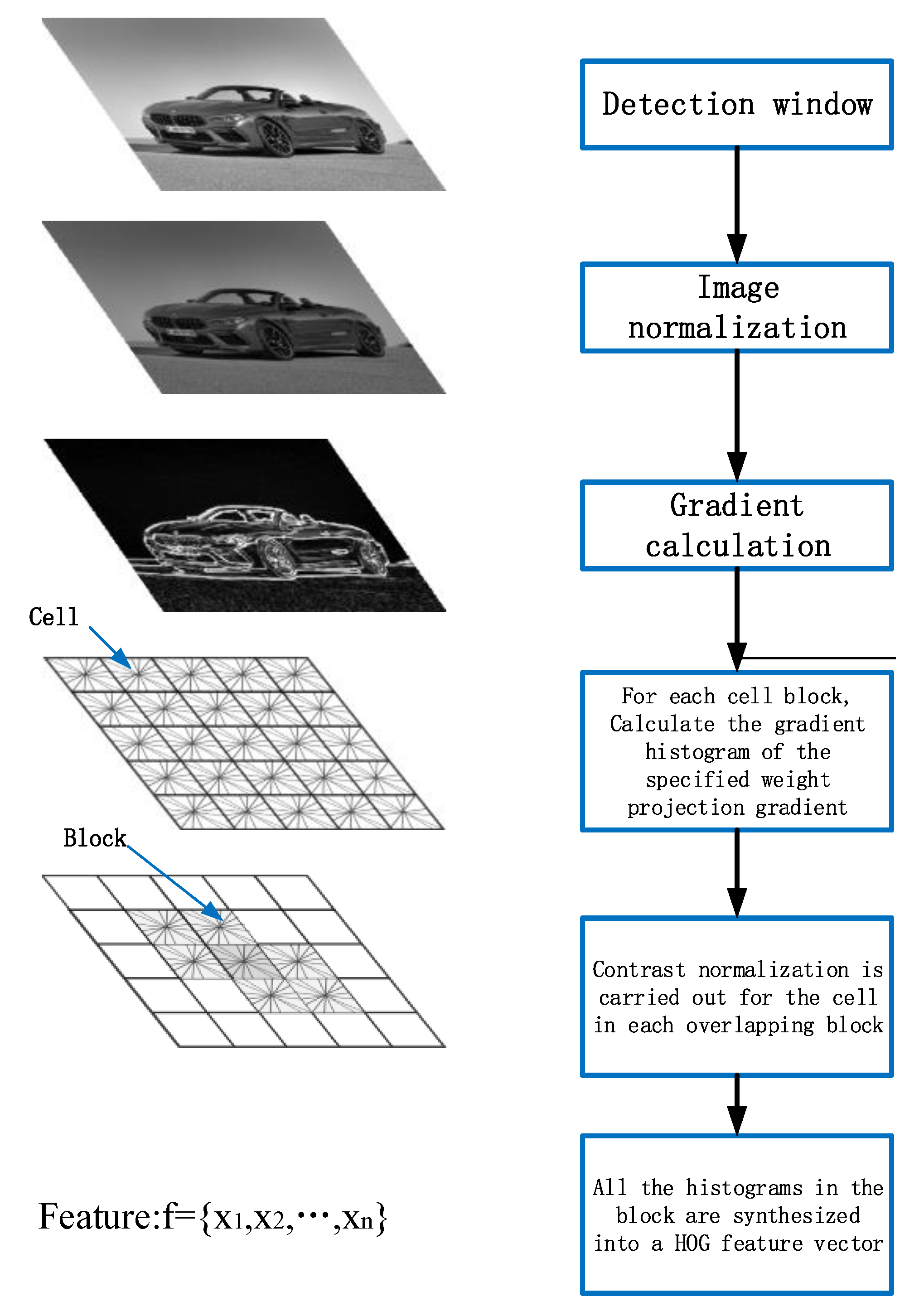
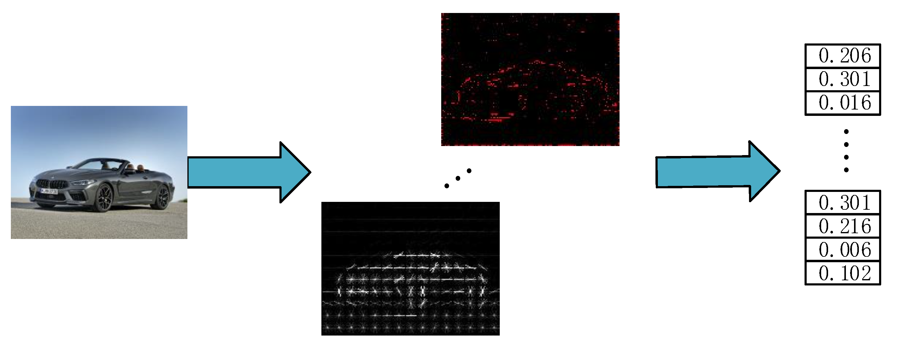
Orientation gradient histogram feature is to use the knowledge of statistics to calculate and statisticize the gradient in different directions of the image block to form the gradient histogram feature. In order to carry out vehicle detection based on multiple features, firstly, HOG feature extraction is needed for the vehicle-detection range. HOG feature is an operator that characterizes a target in the field of machine vision. Figure 1 shows the formation of HOG feature below.
HOG processing is as follows:
In order to reduce the adverse effect of illumination change on image detection, image graying and normalization processing are indispensable. The commonly used three methods of image grayscale are:
1. Component method: one of the three components of R, G, and B of color image is taken as the grayscale image Gray value: Gray = B or Gray = G or Gray = R.
2. Maximum method: the maximum value of the R, G, and B components of the color image is taken as the grayscale value of the grayscale imageMax (R, Max (G, B)).
3. Weighted average method: R, G, and B components of the color image are weighted and average with different weights. Human eyes are most sensitive to green and least sensitive to blue. Image graying Formula (1) is shown as follows:
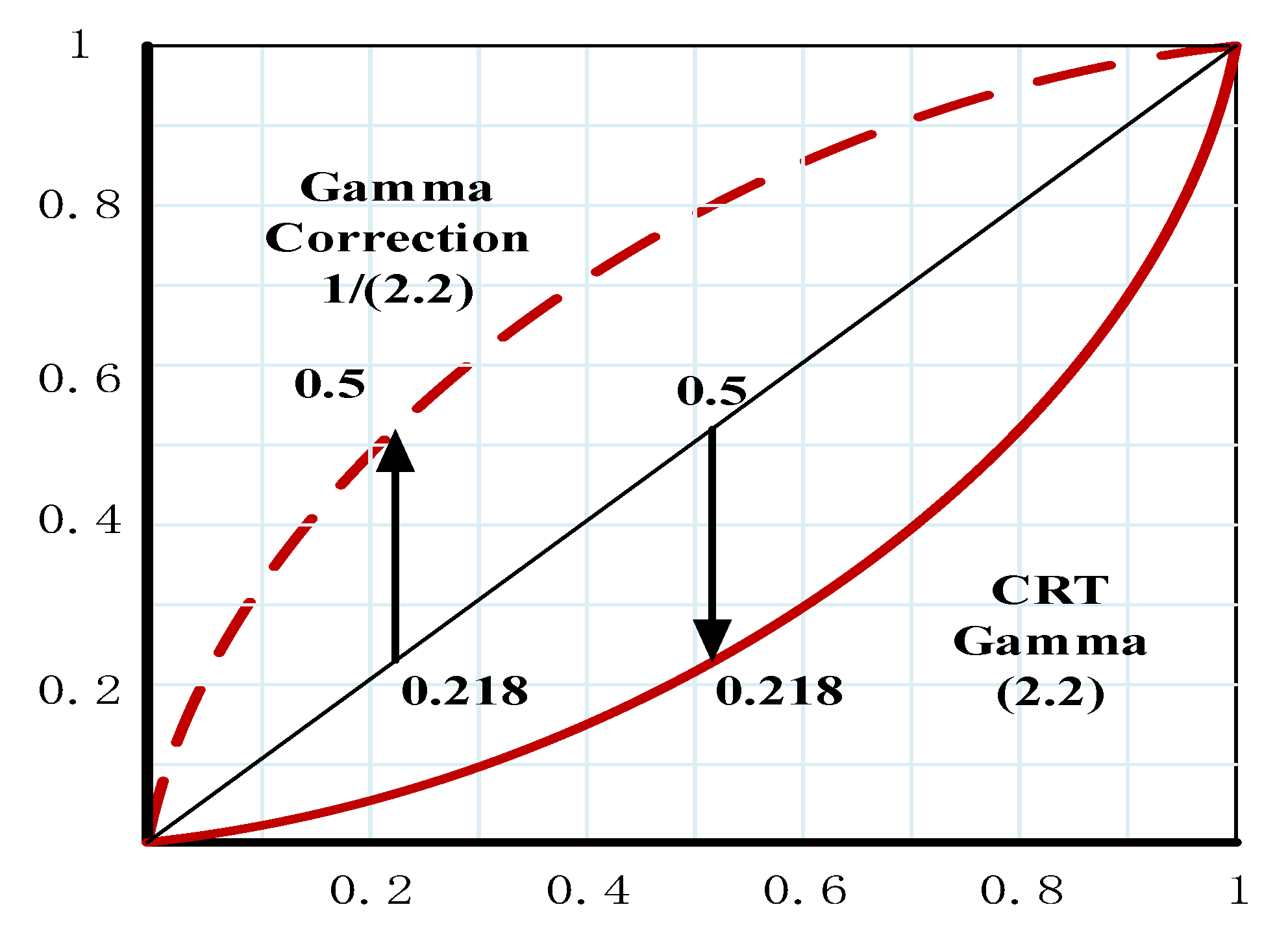
The local area of the surface exposure is a relatively large proportion in the image texture intensity. Therefore, the influence of local shadow and uneven illumination can be effectively reduced by normalization. In the gamma space, the dynamic range will be reduced, the contrast of the image will be reduced, and the gray value of the image will be increased, which make the image brighter overall when the gamma <1. When gamma >1, the dynamic range is reduced within the region of the reduced gray value, the contrast of the image is reduced, the gray value of the image is reduced, and the overall image is faded. The local area of the surface exposure is relatively large proportion in the image texture intensity. Therefore, the influence of local shadow and uneven illumination can be effectively reduced by normalization. The Gamma-correction diagram is shown in Figure 2.
Gamma-compression formula is shown in Formula (2):
In the formula, gamma = 1/2.
After image graying and normalization processing, in order to calculate the vehicle characteristic gradient, it is necessary to calculate the gradient direction value of each pixel. The gradient of pixel point (x, y) in the image is shown in Formula (3):
where , and respectively represent the horizontal gradient, vertical gradient, and pixel value at the input pixel point (x, y).
In order to calculate the magnitude and direction of the gradient of pixel points, the operator [−1,0,1] is usually used to carry out convolution calculation on the original image to obtain the gradient component in the x direction. Then the convolution computation is performed by the operator [−1,0,1] to obtain the gradient component in the y direction. Finally, the gradient size and direction of the pixel point can be obtained as shown in Formula (4):
In order to facilitate the statistical analysis of the calculated feature gradient and reduce the sensitivity of vehicle posture and appearance, the image needs to be segmented into “cell”.
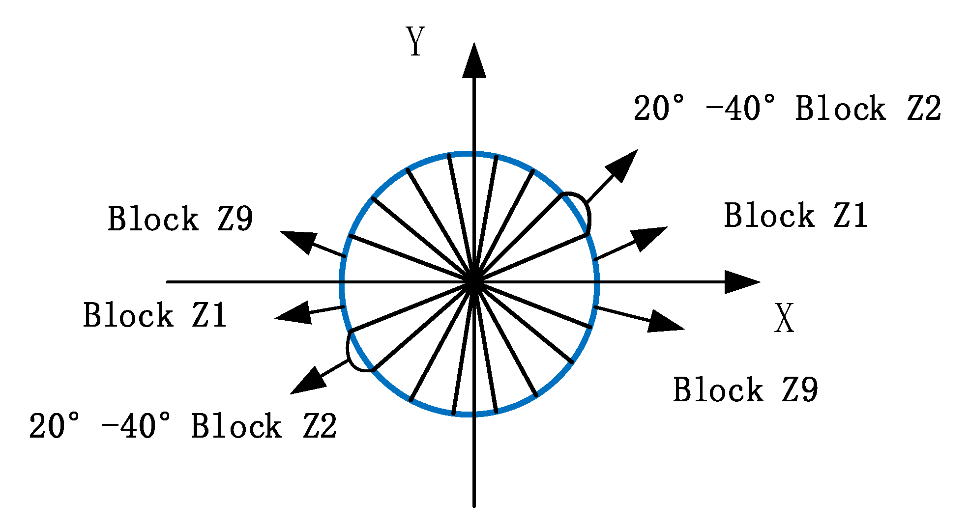
Assuming that the pixel of each cell is 6 × 6, if the histogram of nine bins is used to calculate the information of these cells, the cell is divided into nine blocks with different directions, as shown in Figure 3.
In Figure 3, the gradient direction of each pixel is 0–20 degrees. Add one to the first bin count of the histogram. Then, each pixel point in the cell is weighted and projected as shown above. Finally, the histogram of gradient direction of the whole image can be obtained.
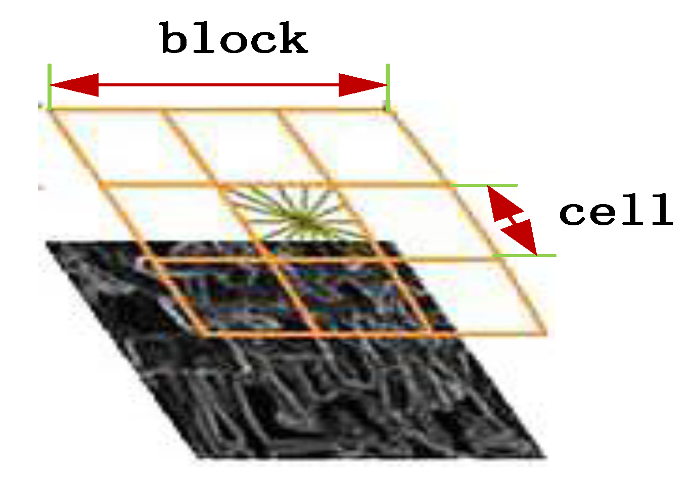
In order to count the segmented cells and reduce the impact of light changes, block synthesis, and normalization processing of cells are employed as shown in Figure 4. The parameters of the feature-description operator in this paper are set as 3 × 3 cells/interval, 6 × 6 pixels/cell, and nine histogram channels.
Finally, in order to obtain the HOG feature of the vehicle, all blocks need to be processed in series. For the image of sample data 64 × 64, it is assumed that 8 × 8 pixels constitute a cell, and a block is composed of 2 × 2 cells. Each cell has nine dimensional features, and each block has 4 × 9 = 36 dimensional features. For the data images obtained from the vehicle camera, assume that each block is used as the detection window to extract features from the regions of dynamic interest, and four pixels are used as the step length. The number of detection windows in the horizontal direction is: (64 − 16)/8 + 1 = 7, and the detection window in the vertical direction is the same as above.
Therefore, the number of detection window features of 64 × 64 is: 36 × 7 × 7 = 1764.
2.1.2. LBP Feature Extraction
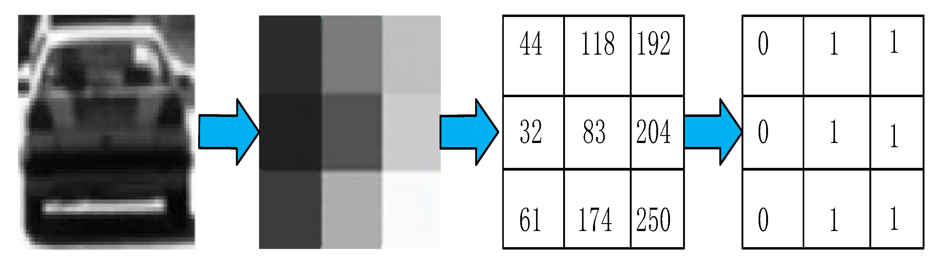
The local-binary-patterns operator is an effective texture-description operator, which has the remarkable advantages of invariance on rotation and gray. The basic idea is to use the gray value of its center pixel as the threshold and compare it with its neighborhood binary code to describe the local texture features. According to the LBP proposed by Song et al. [33], LBP characteristics of vehicles in the vehicle-detection range are extracted. In the statistical histogram based on LBP feature, the local binary mode feature image is divided into N regional blocks, and the histogram of local binary patterns (LBPH) is obtained by extracting the histogram of each regional block in a series. The local binary mode is shown in Figure 5.
The calculation steps of LBP are as follows:
Calculate LBP characteristic image:
where, () is the pixel of the regional center point, is the gray value of the central pixel, and is the gray value of the neighborhood pixel. n is the total number of pixels in the neighborhood. s(x) is shown as follows:
Then, LBP feature image is processed by block processing. In this article, LBP feature images are segmented into 64 blocks of 8 × 8 size. After that, we calculate the LBPH of each feature image and then normalize the LBPH to 1 × NumPatterns. Finally, we arranged each LBPH in order of its space to form the LBP characteristic vector of the image, the size of which is 1 × (NumPatterns × 64).
In order to improve the computational efficiency of LBP feature extraction and ensure the accuracy of vehicle detection, the eigenvalue of equivalent-feature pattern is adopted in this paper, and the eigenvalue is set to 59, namely NumPatterns = 59. Therefore, the total dimension of the feature vector of the image is 59 × 64 = 3776.
2.1.3. Haar-Like Feature Extraction
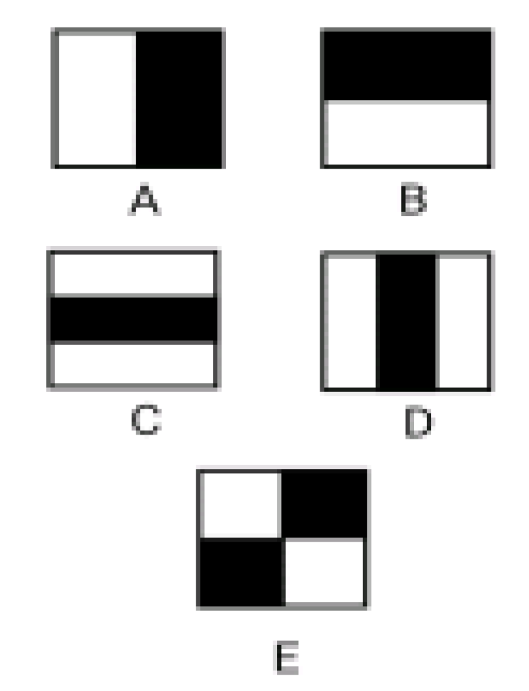
Haar-like feature refers to the value of the rectangular feature (the sum or the difference of all pixel gray values inside two or more rectangles of the same shape and size on the image). License plates, taillights, and rear windshields have prominent rectangular features and obvious gray difference from the surrounding area for vehicles. Therefore, in order to improve the adaptability of feature templates, the feature template shown in Figure 6 is selected in this paper for Haar-like feature calculation.
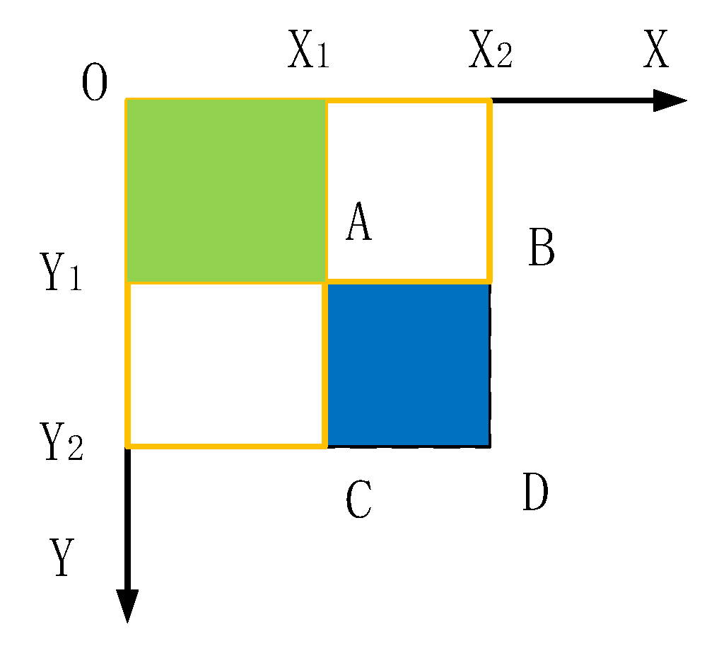
As the size of the image acquired by the detection window is 64 × 64, the number of features of the image exceeds the number of pixels. Therefore, in order to reduce the amount of computation of eigenvalues each time and improve the detection speed, this paper used integral images to calculate eigenvalues, as shown in Figure 7.
As shown in Figure 7 of the integral region, the gray value of region is , the gray value of region is , the gray value of region is , the gray value of region is , and the gray value of ABCD region is V. The calculation Formula (7) is as follows:
2.2. Feature Dimension Reduction and Fusion Processing
Because vehicle-detection method based on a single feature is likely to cause vehicle missed detection and false detection, vehicle detection research based on HOG, LBP, and Haar-like features fusion is carried out in order to improve the accuracy and robustness of vehicle detection.
However, as multifeature fusion will increase the total dimension of vehicle features and reduce the vehicle-detection rate, vehicle-dimension-reduction processing is required in order to reduce the calculation amount of vehicle detection and ensure the real-time performance of vehicle detection.
2.2.1. Feature Dimension Reduction
PCA [36] uses orthogonal transformation to transform correlated variables in the data set into unrelated principal-component components, so as to delete noise in the data set and achieve the purpose of dimensionality reduction. PCA has the advantage of using fewer data dimensions to retain more original data-point characteristics. Therefore, in order to reduce vehicle-feature dimensions and retain as many vehicle features as possible, PCA dimension-reduction processing is adopted.
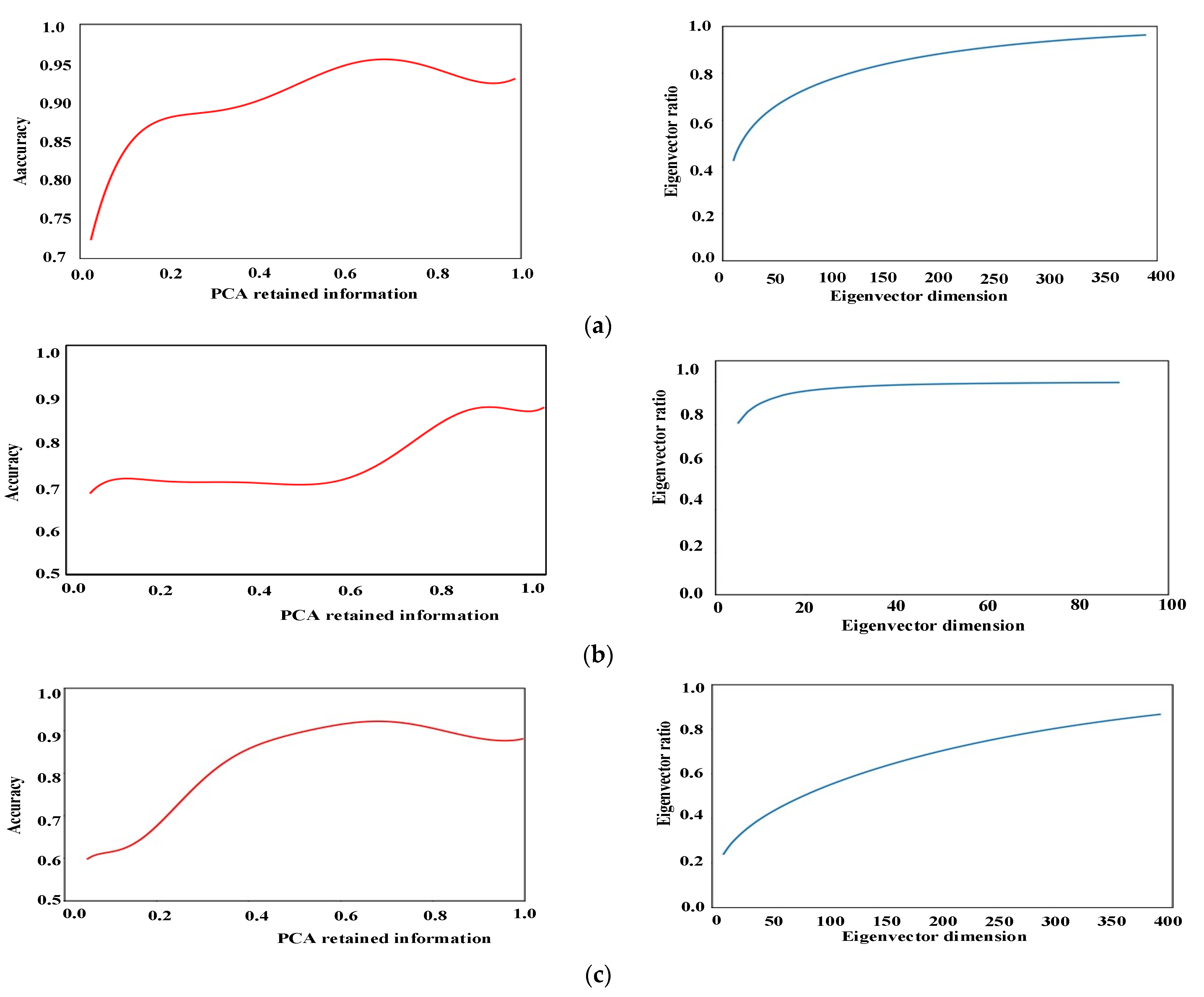
PCA achieves the effect of dimension reduction for the data by calculating the eigenvectors corresponding to the maximum eigenvalue of the covariance matrix of the data set to find the directions with the maximum data variance. The analysis results of PCA for HOG, LBP, and Haar-like features can be seen in Figure 8.
The vehicle images from the front view, rear view, and side view are taken as positive samples, while signs, buildings, roads, and sky are taken as negative samples. Then HOG, LBP, and Haar-like features extracted from the data of positive and negative samples were respectively taken as inputs to obtain corresponding eigenvalues and corresponding feature spaces.
According to Mao [36], when calculating , is used in this paper. If , extract the first principal components . The dimensionless feature data can be obtained by projecting the above features into the corresponding feature subspace.
HOG, LBP, and Haar-like features extracted from positive and negative samples were analyzed respectively to obtain the feature vector dimension of PCA.
The analysis results show that HOG, LBP, and Haar-like features can ensure good accuracy when information is retained in a proportion of 0.71, 0.73, and 0.86, respectively, according to which we select the information dimension characteristics for vehicle detection.
2.2.2. Feature Fusion
In order to improve the accuracy of vehicle detection further, feature-level fusion processing for the vehicle characteristics is conducted after PCA dimensionality-reduction processing. The fusion refers to the concatenation of a single feature of all sublevels, and finally the fusion feature obtained is the sum of the dimensions of all sublevel features.
For the acquired vehicle image features, the obtained-feature matrix is transformed into feature vectors first, then all feature vectors are serialized, and the calculation Formula (8) is shown as follows:
In the above equation, is the feature after fusion, and α and β are the subfeatures before fusion. The extracted HOG, LBP, and Haar-like features are fused visually, as shown in Figure 9.
2.3. Design and Training of Classifier
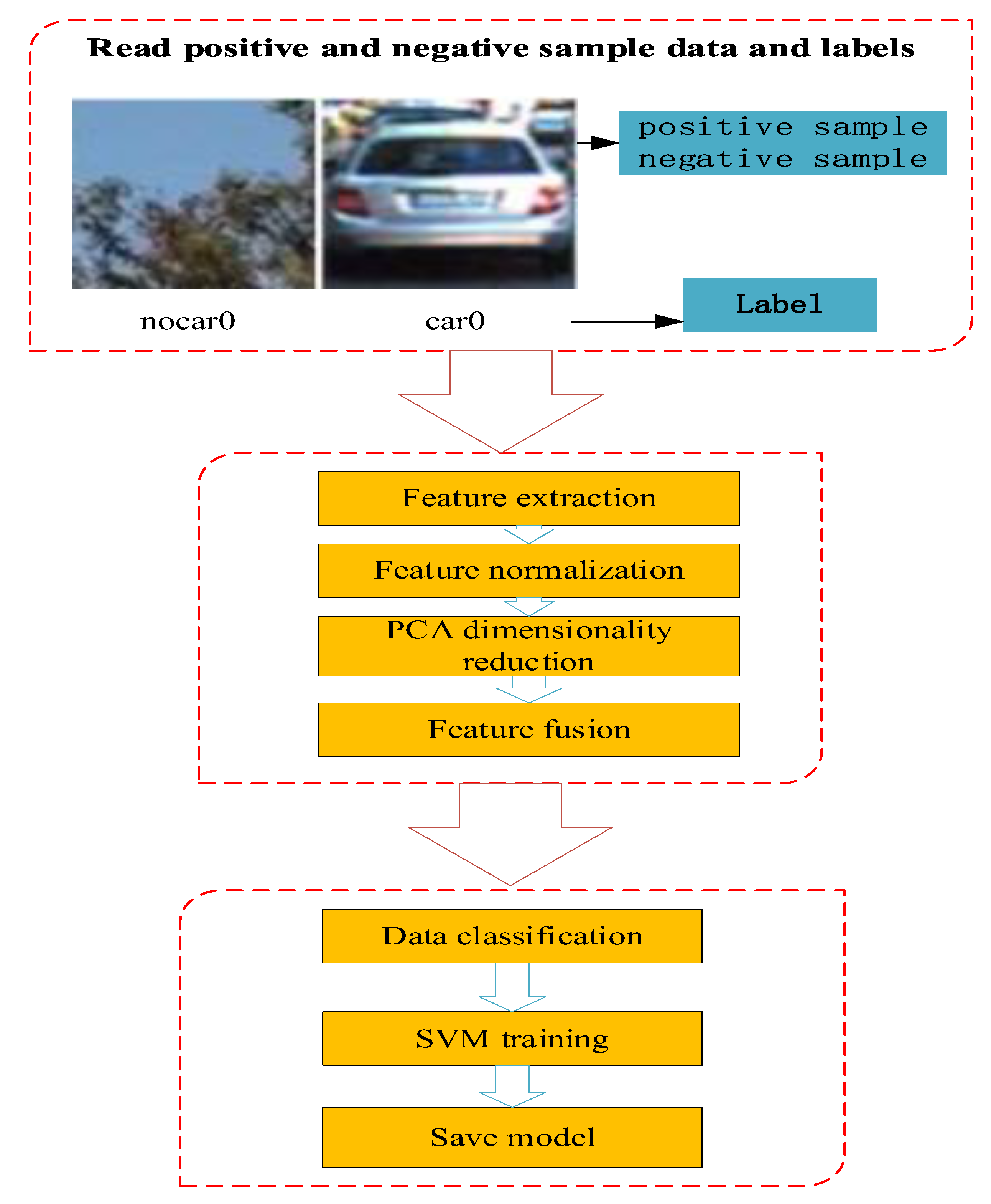
After obtaining the characteristics of the required samples, corresponding classifiers should be built to select and identify the extracted vehicle characteristics. SVM classifier, with the ability to catch key samples and eliminate redundant samples, is adopted to detect and classify vehicles in front. The detection and classification process is shown in Figure 10.
The SVM classifier training process is as follows:
After obtaining the positive and negative sample data sets respectively, a linear kernel function is taken as the kernel due to its relative advantages after relevant tests [37], and a SVM vehicle-classifier model based on multiple features is established. In addition, the algorithm performs traversal parameter combination through GridSearchCV and determines the best effect parameters through five-fold crossvalidation.
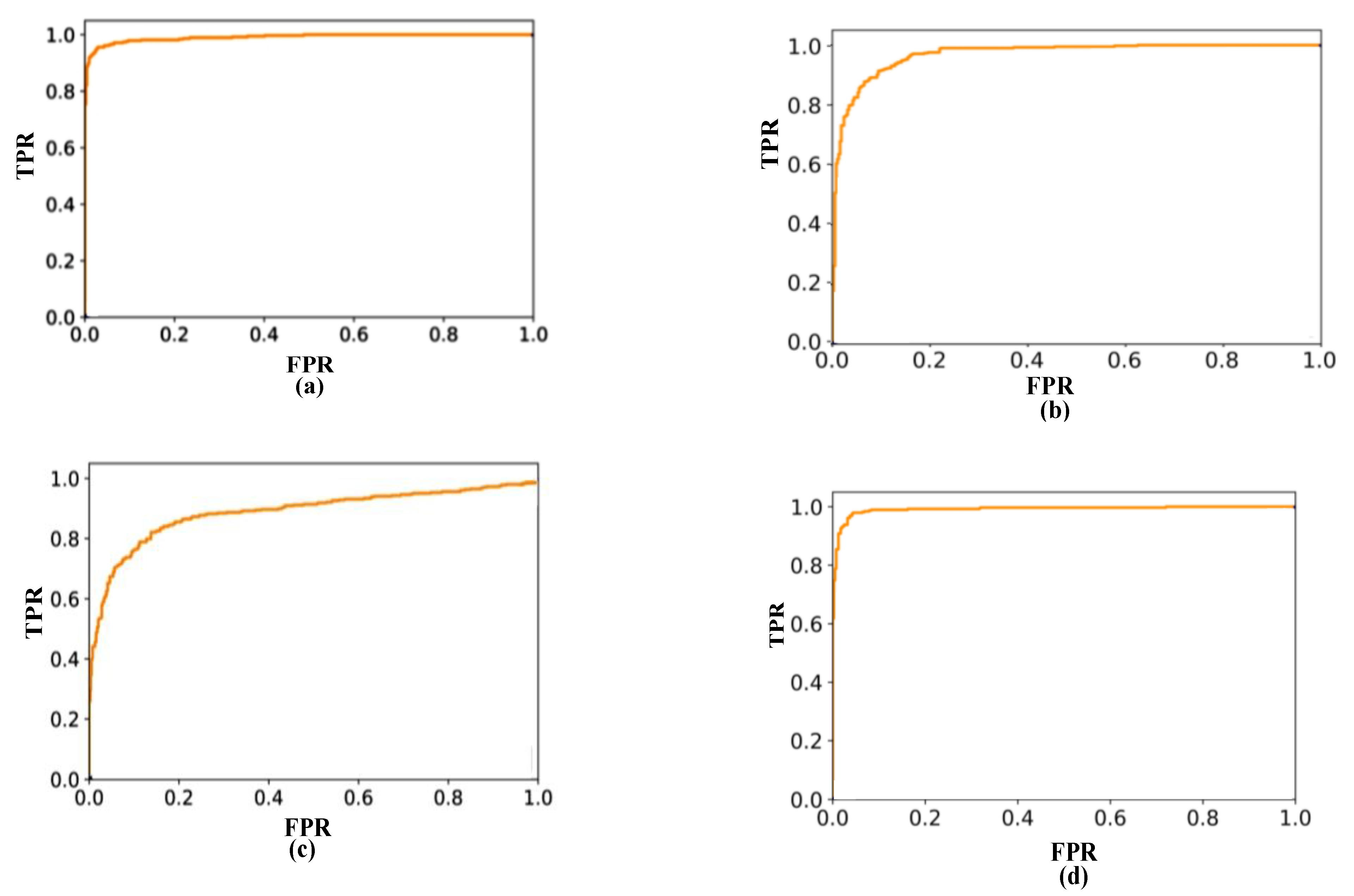
After a training data set of positive and negative samples as the input of support vector-machine classifier, finally, a classifier model with excellent classification performance is obtained, and the receiver operating characteristic curve (ROC) of the model is shown in Figure 11.
The area enclosed by the curve is defined as AUC (area under curve). The larger the area of AUC, the better the effect of the classifier. According to the above experimental results, the AUC enclosed by LBP, HOG, Haar-like, and multifeature ROC was 0.969, 0.976, 0.913, and 0.992.
The results show that the multifeature fusion-classifier model has a relatively excellent classification performance.
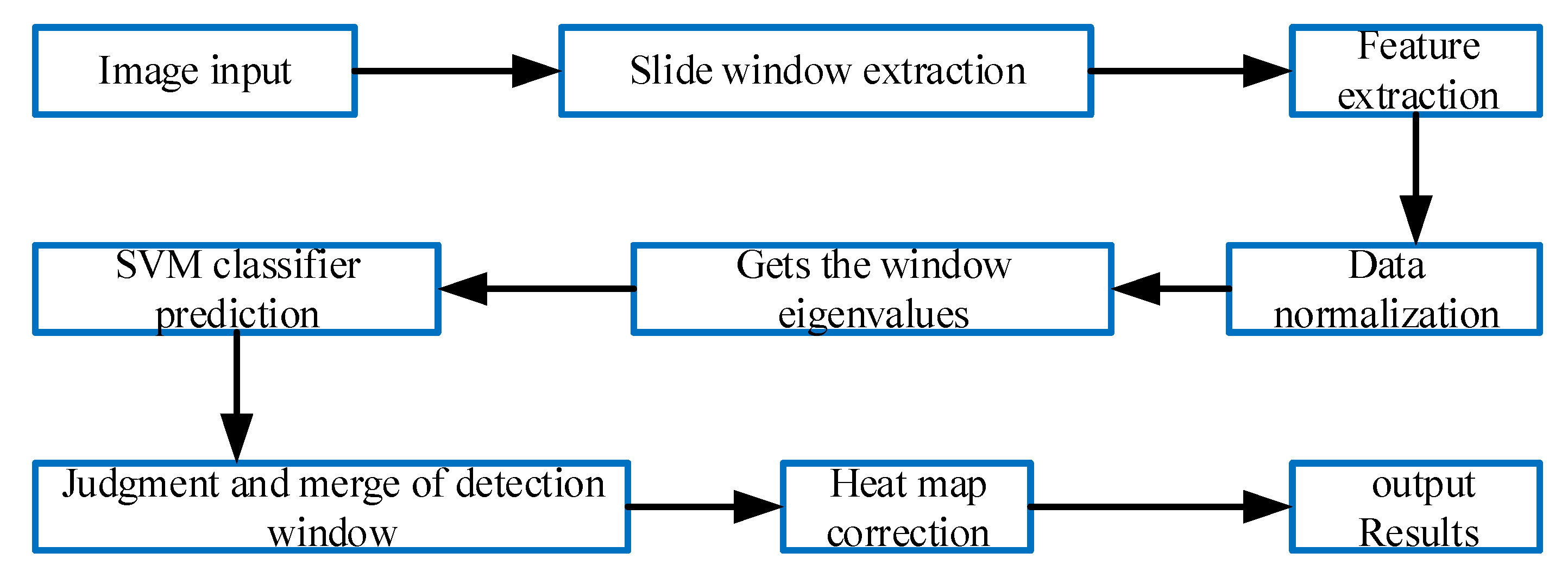
2.4. Experimental Test and Results
To verify the proposed algorithm, we use the function interface of Python 3.5 related libraries (numpy, cv2, matplotlib, and sklearn) to carry out corresponding tests on the above training algorithm under the compiling environment of Spyder (Anaconda). The relevant configuration of the PC used during the test was Inter Core (TM) I7-8700 CPU 3.20 GHz and 16 GB of memory. The related process of the detection is shown in Figure 12.
2.4.1. Experimental Evaluation
In order to make a reasonable and effective evaluation of the test results, the test results were counted and compared with other methods. Then, the accuracy and omission rate were employed to evaluate and analyze the detection results.
Intersection over union (IoU) was employed to measure the coincidence degree of the same area in the evaluation of target detection. The IoU ratio refers to the ratio of intersection and union. Its definition is shown in Formula (9).
where D represents the predicted region and G represents the marked region. The prediction is considered correct when the intersection ratio is greater than 0.5.
True positive (TP), false negative (FN), and false positive (FP) are commonly used indicators in the evaluation of machine learning [38]. According to these indicators, precision P, omission rate O and error rate R are calculated respectively, the P, O, and R are defined as follows.
P = TP/(TP + FP)
R = 1−TP/(TP + FP)
O = 1−TP/(TP + FN)
2.4.2. Test Results
Based on some data collected from BDD [39], Udacity, and the network, this paper selected 1200 pieces of data in good driving environments and complex driving environments, with the size of 1280 × 720 to train the classifier and 600 pieces each to test the vehicle detection classifier.
Moreover, in order to verify the performance of this algorithm, the detection results of multifeature-fusion algorithm and the current mainstream detection algorithm are compared (Table 1 and Table 2).
The parameters of gridsearchCV are shown below:
GridSearchCV (estimator = classifier, param_grid = parameters, scoring = ‘accuracy’, cv = 10, n_jobs = −1), parameters = [{‘C’: [1, 10, 100, 1000], ‘kernel’: [‘linear’]}, ‘gamma’: [0.1, 0.15, 0.2, 0.25, 0.3, 0.35, 0.4, 0.45, 0.5, 0.55, 0.6, 0.65, 0.7, 0.75, 0.8, 0.85, 0.9]}], accuracy = accuracy_score (y_test, y_pred), classifier = svc (kernel = ’linear’, gamma = 0.7), the best parameters of classifier is: ’C’: 1, ’gamma’: 0.7
As can be seen from Table 1 and Table 2, compared with the detection methods in literature [40,41,42], the multifeature-fusion vehicle-detection method used in this paper possesses the best accuracy in vehicle detection in a good driving environment, and the omission rate is relatively reduced at only 2.15%.
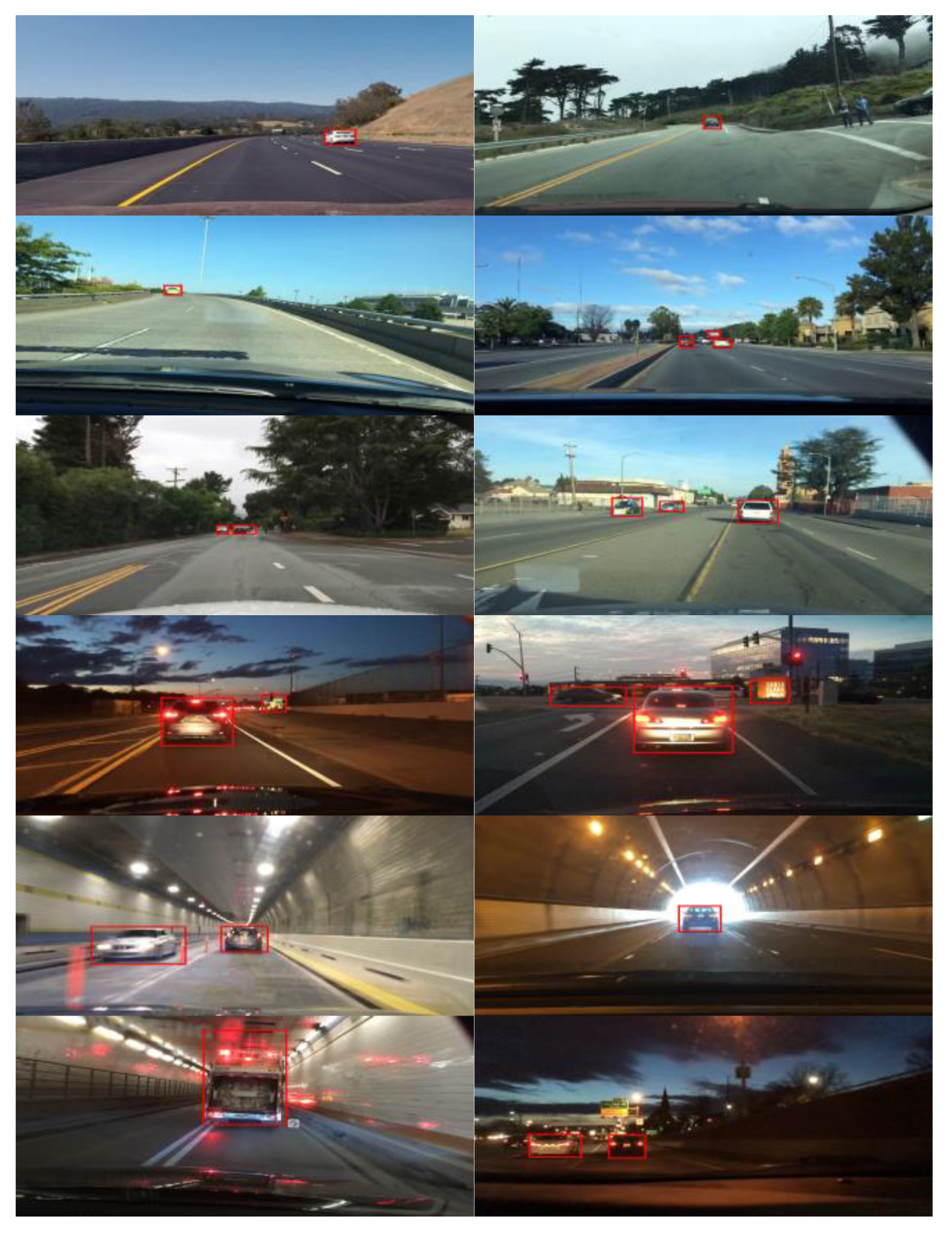
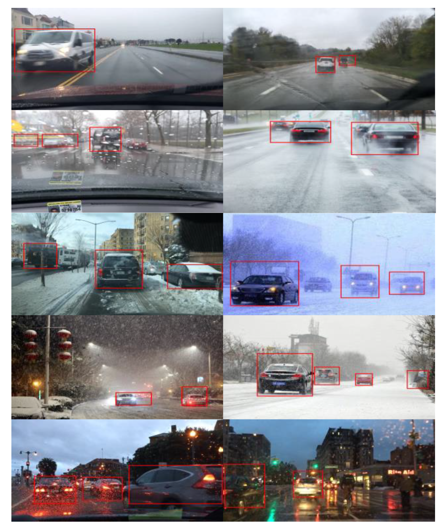
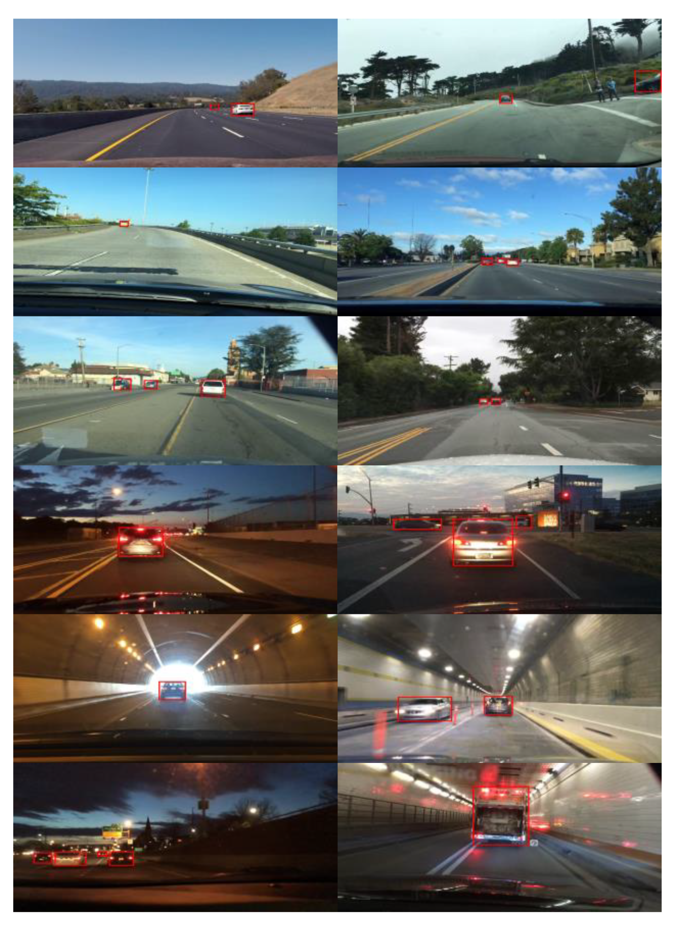
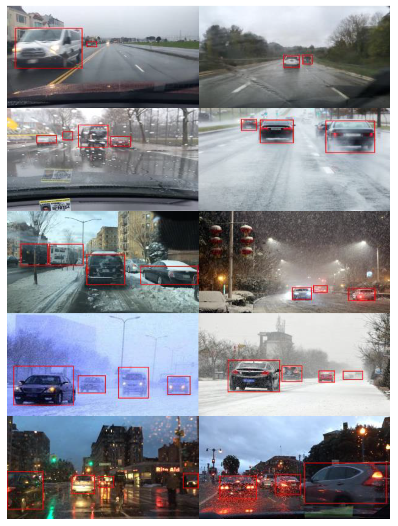
From Figure 13 and Figure 14, the multifeature vehicle-detection method shows good detection performance in a good traffic environment, such as light in good condition, the highway, simple tunnel, etc. While in complex traffic scenes such as bad lighting conditions, blizzard, rainy day, the vehicle-detection classifier tends to produce misjudgment, which causes error rate to rise, because these environments are prone to contain some similar texture with cars and contour features of illusion. However, compared with other methods, the test method shows better stability.
3. Cascade Vehicle Detection Based on CNN
Based on the test results above, in the good driving environment, multifeature method proposed presents a good detection performance. However, in heavy snow, rainy days and other environments, it is easy to generate false features such as car texture and contour, which makes the vehicle-detection classifier misjudge.
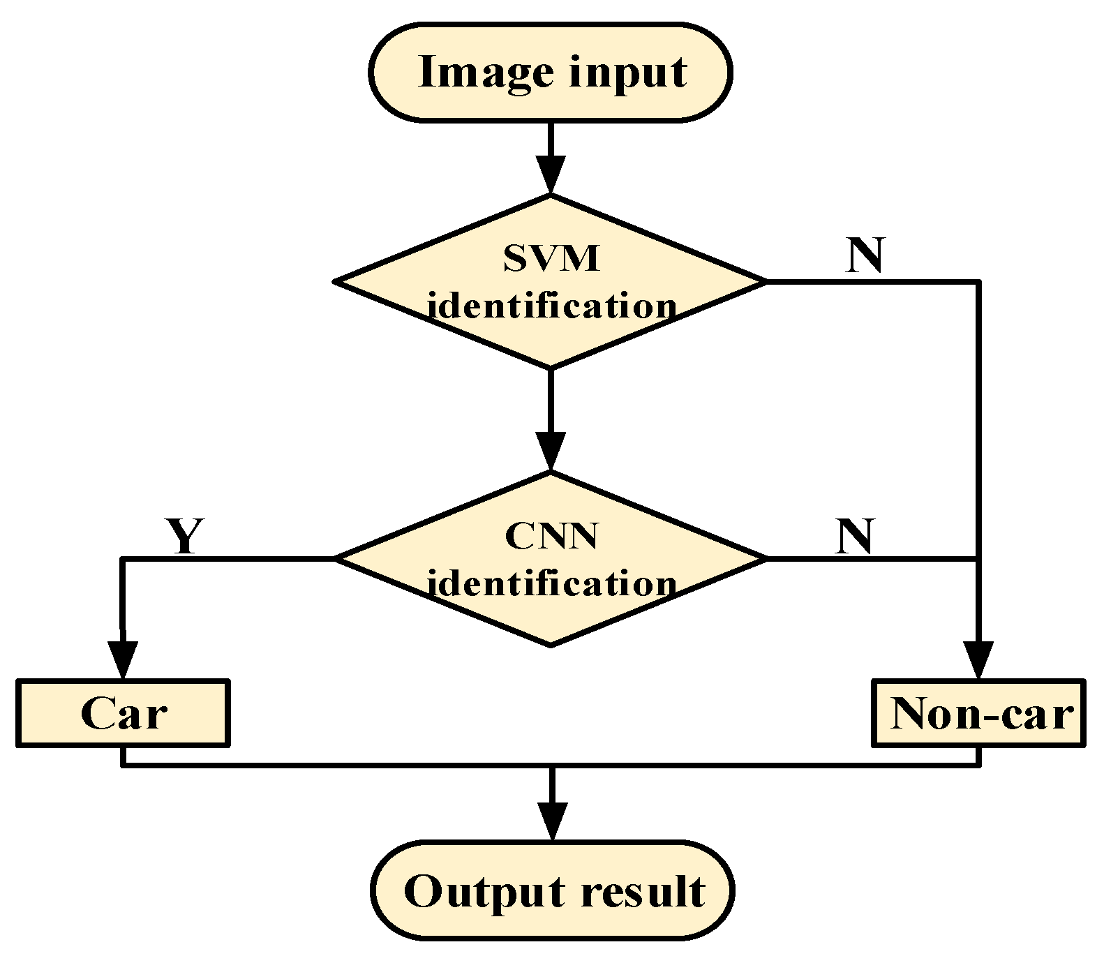
Therefore, in order to improve the accuracy and robustness of vehicle detection further, a cascading-detection architecture based on CNN is established through which nonvehicle windows are excluded using SVM, and the remaining detection windows are identified based on CNN model (as shown in Figure 15).
3.1. VGG16 Neural-Network-Model Construction
The structure of the convolutional neural network includes input layer, multilayer convolutional layer, pooling layer, full connection layer, and output layer. Compared with other convolutional-neural-network models, VGG16 [43] possesses the advantages of few parameters, simple calculations, and high accuracy. Therefore, in order to improve the accuracy and real-time performance of vehicle-validation cascade detection, this paper constructed VGG16 for cascade-verification detection.
VGG16 network structure has a total of 16 layers, which is mainly composed of 13 convolutional layers and three full-connection layers. The convolutional-neural-network architecture adopts the structure: CNN = convolution + convolution + convolution + pooling. With the capability to reduce the number of parameters, VGG16 not only prevent overfitting but also make the network deep enough. The network structure can reduce the computation complexity well because the pooling operation does not participate in the parameter computation.
Therefore, after obtaining the screening windows of SVM, VGG16 will be used for cascade detection of those vehicle windows whose prediction probability is between the boundary threshold to further improve the accuracy of detection.
3.2. Design of Cascade-Detection Confidence of Vehicles
Before cascade-vehicle detection, in order to further improve the accuracy and robustness of vehicle detection, this paper selects the detection window based on multifeature-fusion vehicle detection and uses probability-prediction function to predict the features in the detection window, that is, the confidence of the detection window.
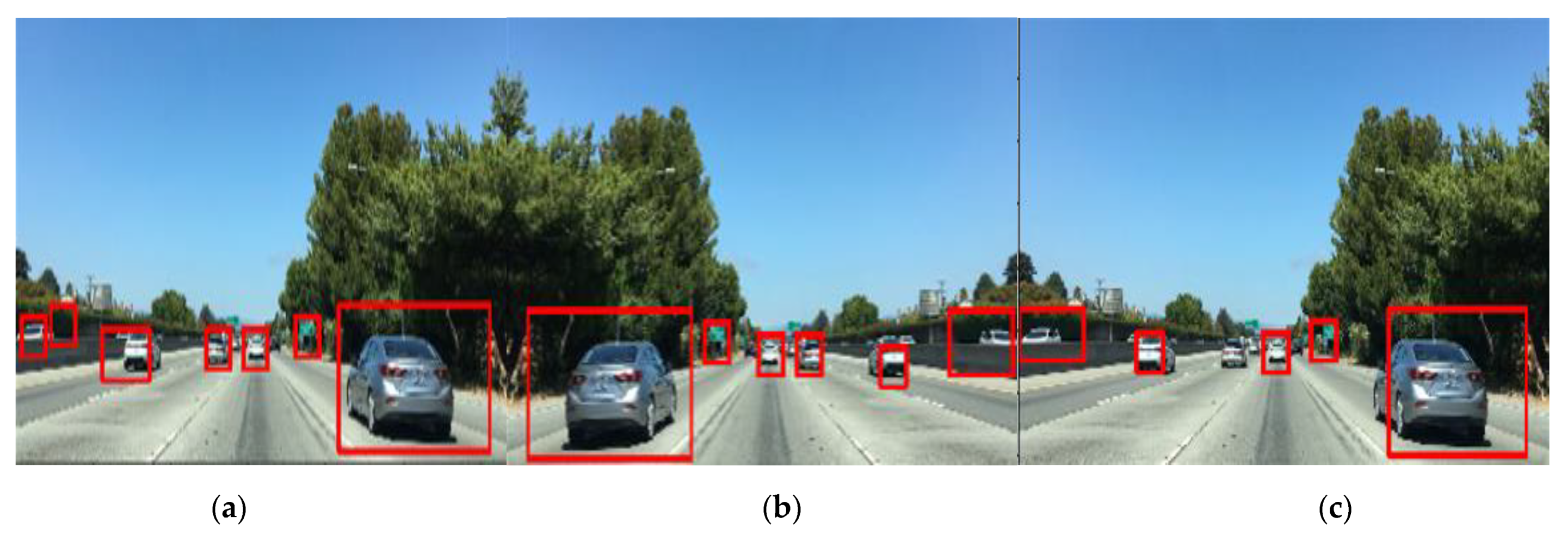
Under different probability predicted values, the results of vehicles and nonvehicle targets detected by the test images are different, and with the continuous improvement of probability-predicted values (confidence), the accuracy of vehicle detection will be relatively improved, but the omission rate of vehicles will also increase. Therefore, in order to reduce omission rate of vehicles and ensure vehicles recall rate in complex traffic environment at the same time, we need to verify the determination of cascade confidence probability forecast. According to the different test, this article chose 0.88 as preliminary vehicle recognition based on feature fusion of confidence, and relevant probability-prediction results shown in Figure 16, as follows.
CNN validation cascade classifier proposed is tested with the integrated data set which is mainly divided into good weather (600 pieces), rainy, and night data sets (600 pieces). Vehicle-detection method based on multifeature fusion SVM and CVDM-CNN are compared in the test. The experimental results are shown in Table 3 and Table 4, and the detection effect is shown in Figure 17 and Figure 18.
As can be seen in Table 3 and Table 4, compared with the multifeature-fusion algorithm proposed in this paper under the good environment and complex environment, the cascade method omission rate is reduced by 0.78% and 0.99%, respectively. The recall is also improved by 0.88% and 1.59%, indicating that cascade-vehicle detection based on CNN method shows good robustness and accuracy.
4. Conclusions
To improve the accuracy and robustness of vehicle detection in complex driving environment, a cascade vehicle detection method base on CNN is presented.
After LBP, Haar-like, and HOG features extraction, PCA dimension reduction and feature fusion processing are carried out for vehicle detection range. Then, the detection range is filtered by SVM classifier based on multifeature fusion, and the filtered detection box is taken as the input of CNN detection, and the cascade detection is put forward.
In order to verify the accuracy and robustness of the method used, and the recall of this article reached 98.69% in a good driving environment. In addition, when the detection is in a complex driving environment, the false-detection rate and omission rate of the cascade vehicle-detection method based on CNN decreased by 1.37% and 0.7%, respectively. Compared with other mainstream vehicle-detection methods, the cascade vehicle-detection algorithm shows good accuracy and better robustness.
Author Contributions
Conceptualization, J.H. and Y.S.; methodology, S.X.; software, S.X.; validation, J.H., Y.S., and S.X.; formal analysis, S.X.; investigation, Y.S.; resources, Y.S.; writing—original draft preparation, Y.S.; supervision, J.H.; data curation, J.H.; writing—review and editing, J.H.; All authors have read and agreed to the published version of the manuscript.
Funding
This research received no external funding.
Conflicts of Interest
The authors declare no conflict of interest.
References
- Private Car Ownership in China in 2019. 2020. Available online: http//www.askci.com/news/chanye/20200107/1624461156140.shtml (accessed on 7 January 2020).
- Batavia, P.H.; Pomerleau, D.A.; Thorpe, C.E. Overtaking Vehicle Detection Using Implicit Optical Flow. In Proceedings of the Conference on Intelligent Transportation Systems, Boston, MA, USA, 12 November 1997. [Google Scholar]
- Shi, L.; Deng, X.; Wang, J.; Chen, Q. Multi-target Tracking based on optical flow method and Kalman Filter. Comput. Appl. 2017, 37, 131–136. [Google Scholar]
- Gao, L. Research on Detection and Tracking Algorithm of Moving Vehicle in Dynamic Scene Based on Optical Flow. Ph.D. Thesis, University of Science and Technology of China, Hefei, China, 2014. [Google Scholar]
- Hu, X.; Liu, Z. Improved Vehicle Detection Algorithm based on Gaussian Background Model. Comput. Eng. Des. 2011, 32, 4111–4114. [Google Scholar]
- Fu, D. Research on Vehicle Detection Algorithm based on Background Modeling. Ph.D. Thesis, University of Science and Technology of China, Hefei, China, 2015. [Google Scholar]
- Yang, H.; Qu, S. Real-Time Vehicle Detection and Counting in Complex Traffic Scenes Using Background Subtraction Model with Low-Rank Decomposition. IET Intell. Transp. Syst. 2018, 12, 75–85. [Google Scholar] [CrossRef]
- Kato, T.; Ninomiya, Y.; Masaki, I. Preceding Vehicle Recognition Based on Learning from Sample Images. IEEE Trans. Intell. Transp. Syst. 2002, 3, 252–260. [Google Scholar] [CrossRef]
- Satzoda, R.K.; Trivedi, M.M. Multipart Vehicle Detection Using Symmetry-Derived Analysis and Active Learning. IEEE Trans. Intell. Transp. Syst. 2016, 17, 926–937. [Google Scholar] [CrossRef]
- Broggi, A.; Cerri, P.; Antonello, P.C. Multi-Resolution Vehicle Detection Using Artificial Vision. In Proceedings of the IEEE Intelligent Vehicles Symposium, Parma, Italy, 14–17 June 2004. [Google Scholar]
- Lee, B.; Kim, G. Robust detection of preceding vehicles in crowded traffic conditions. Int. J. Automot. Technol. 2012, 13, 671–678. [Google Scholar] [CrossRef]
- Li, L.; Deng, Y.; Rao, X. Application of color feature Model in static vehicle detection. J. Wuhan Univ. Technol. 2015, 37, 73–78. [Google Scholar]
- Kutsuma, Y.; Yaguchi, H.; Hamamoto, T. Real-Time Lane Line and Forward Vehicle Detection by Smart Image Sensor. In Proceedings of the IEEE International Symposium on Communications and Information Technology, Sapporo, Japan, 26–29 October 2004. [Google Scholar]
- Han, S.; Han, Y.; Hahn, H. Vehicle Detection Method using Haar-like Feature on Real Time System. Chemistry 2009, 15, 9521–9529. [Google Scholar]
- Mohamed, E.H.; Sara, E.; Ramy, S. Real-Time Vehicle Detection and Tracking Using Haar-like Features and Compressive Tracking; Springer: Berlin, Germany, 2014. [Google Scholar]
- Neumann, D.; Langner, T.; Ulbrich, F.; Spitta, D.; Goehring, D. Online Vehicle Detection Using Haar-Like, Lbp and Hog Feature Based Image Classifiers with Stereo Vision Preselection. In Proceedings of the 2017 28th IEEE Intelligent Vehicles Symposium, Los Angeles, CA, USA, 11–14 June 2017. [Google Scholar]
- Du, T.; Tihong, R.; Wu, J.; Fan, J. Vehicle recognition method based on Haar-like and HOG feature combination in traffic video. J. Zhejiang Univ. Technol. 2015, 43, 503–507. [Google Scholar]
- Li, X.; Guo, X. A HOG Feature and SVM Based Method for Forward Vehicle Detection with Single Camera. In Proceedings of the 2013 5th International Conference on Intelligent Human-Machine Systems and Cybernetics, Hangzhou, China, 26–27 August 2013; pp. 263–266. [Google Scholar]
- Li, Z.; Liu, W. A Moving vehicle Detection Method Based on Local HOG Feature. J. Guangxi Norm. Univ. 2017, 35, 1–13. [Google Scholar]
- Lei, M.; Xiao, Z.; Cui, Q. Real-time detection of forward vehicles based on two features. J. Tianjin Norm. Univ. 2010, 30, 23–26. [Google Scholar]
- Ma, W.; Miao, Z.; Zhang, Q. Vehicle classification based on multi-feature fusion. In Proceedings of the 5th IET International Conference on Wireless, Mobile and Multimedia Networks (ICWMMN 2013), Beijing, China, 22–25 November 2013; pp. 215–219. [Google Scholar]
- Haselhoff, A.; Kummert, A. A Vehicle Detection System Based on Haar and Triangle Features. In Proceedings of the 2009 IEEE Intelligent Vehicles Symposium, Xi’an, China, 3–5 June 2009. [Google Scholar]
- Girshick, R.; Donahue, J.; Darrell, T.; Malik, J. Region-Based Convolutional Networks for Accurate Object Detection and Segmentation. IEEE Trans. Pattern Anal. Mach. Intell. 2016, 38, 142–158. [Google Scholar] [CrossRef]
- He, K.; Zhang, X.; Ren, S.; Sun, J. Spatial Pyramid Pooling in Deep Convolutional Networks for Visual Recognition. IEEE Trans. Pattern Anal. Mach. Intell. 2015, 37, 1904–1916. [Google Scholar] [CrossRef] [PubMed] [Green Version]
- Girshick, R. Fast R-Cnn. In Proceedings of the 2015 IEEE International Conference on Computer Vision, Las Condes, Chile, 11–18 December 2015. [Google Scholar]
- Ren, S.; He, K.; Girshick, R.; Sun, J. Faster R-Cnn: Towards Real-Time Object Detection with Region Proposal Networks. IEEE Trans. Pattern Anal. Mach. Intell. 2017, 39, 1137–1149. [Google Scholar] [CrossRef] [Green Version]
- Redmon, J.; Divvala, S.; Girshick, R.; Farhadi, A. You only Look Once: Unified, Real-Time Object Detection. In Proceedings of the 2016 IEEE Conference on Computer Vision and Pattern Recognition, Las Vegas, NV, USA, 26 June–1 July 2016. [Google Scholar]
- Liu, W.; Anguelov, D.; Erhan, D.; Szegedy, C.; Reed, S.; Fu, C.-Y.; Berg, A.C. SSD: Single Shot Multibox Detector. In European Conference Computer Vision; Leibe, B., Matas, J., Sebe, N., Welling, M., Eds.; Springer: Cham, Switzerland, 2016. [Google Scholar]
- Kong, D.; Huang, J.; Sun, L.; Zhong, Z.; Sun, Y. Front vehicle detection algorithm in multi-lane complex environment. J. Henan Univ. Sci. Technol. 2018, 39, 25–30. [Google Scholar]
- Liu, T.; Zheng, N.N.; Zhao, L.; Cheng, H. Learning Based Symmetric Features Selection for Vehicle Detection. In Proceedings of the IEEE Proceedings. Intelligent Vehicles Symposium, Las Vegas, NV, USA, 6–8 June 2005. [Google Scholar]
- Cheng, W.; Yuan, W.; Zhang, M.; Li, Z. Recognition of front vehicle and longitudinal vehicle distance Detection based on tail edge features. Mech. Des. Manuf. 2017, 152–156. [Google Scholar] [CrossRef]
- Laopracha, N.; Sunat, K. Comparative Study of Computational Time That HOG-Based Features Used for Vehicle Detection; Springer: Berlin, Germany, 2018. [Google Scholar]
- Song, X.; Wang, W.; Zhang, W. Vehicle detection and tracking based on LBP texture and Improved Camshift Operator. J. Hunan Univ. 2013, 40, 52–57. [Google Scholar]
- Zhang, X.; Fang, T.; Li, Z.; Dong, M. Vehicle Recognition Technology Based on Haar-like Feature and AdaBoost. J. East China Univ. Sci. Technol. 2016, 260–262. [Google Scholar] [CrossRef]
- Kim, M.S.; Liu, Z.; Kang, D.J. On Road Vehicle Detection by Learning Hard Samples and Filtering False Alarms from Shadow Features. J. Mech. Sci. Technol. 2016, 30, 2783–2791. [Google Scholar] [CrossRef]
- Mao, W. Research on Feature Extraction and Target Tracking Algorithm based on Support Vector Machine. Ph.D. Thesis, Chongqing University, Chongqing, China, 2014. [Google Scholar]
- Gaopan, C.; Meihua, X.; Qi, W.; Aiying, G. Front vehicle detection method based on monocular vision. J. Shanghai Univ. 2019, 25, 56–65. [Google Scholar]
- Liu, R. Research on Video Target Detection Based on Deep learning. Ph.D. Thesis, South China University of Technology, Guangzhou, China, 2019. [Google Scholar]
- BDD-100K. 2018. Available online: https://bair.berkeley.edu/blog/2018/05/30/bdd/ (accessed on 30 May 2018).
- Cao, X.; Wu, C.; Yan, P.; Li, X. Linear SVM classification using boosting HOG features for vehicle detection in low-altitude airborne videos. In Proceedings of the 2011 18th IEEE International Conference on Image Processing, Brussels, Belgium, 11–14 September 2011. [Google Scholar]
- Meng, J.; Liu, J.; Li, Q.; Zhao, P. Vehicle Detection Method Based on Improved HOG-LBP[A]. Wuhan Zhicheng Times Cultural Development Co. In Proceedings of the 3rd International Conference on Vehicle, Mechanical and Electrical Engineering (ICVMEE 2016), Wuhan, China, 30–31 July 2016; Available online: https://www.dpi-proceedings.com/index.php/dtetr/article/viewFile/4861/4490 (accessed on 14 February 2021).
- Jabri, S.; Saidallah, M.; El Alaoui, A.E.B.; El Fergougui, A. Moving Vehicle Detection Using Haar-Like, Lbp and a Machine Learning Adaboost Algorithm. In Proceedings of the 2018 IEEE International Conference on Image Processing, Applications and Systems (IPAS), Sophia Antipolis, France, 12–14 December 2018. [Google Scholar]
- Simonyan, K.; Zisserman, A. Very Deep Convolutional Networks for Large-Scale Image Recognition. arXiv 2014, arXiv:1409.1556. [Google Scholar]
Figure 1.
Orientation gradient histogram feature (HOG) processing.

Figure 2.
Gamma-correction diagram.

Figure 3.
Diagram of cell segmentation.

Figure 4.
Block-composition diagram.

Figure 5.
Local binary pattern diagram.

Figure 6.
Haar-like feature templates.

Figure 7.
Schematic diagram of rectangular pixels and calculation.

Figure 8.
Characteristic dimension analysis. (a) Retained information and eigenvector analysis of HOG after PCA, (b) retained information and eigenvector analysis of Harr after PCA, (c) retained information and eigenvector analysis of local binary pattern (LBP) after principal component analysis (PCA).

Figure 9.
Feature-fusion process.

Figure 10.
Support vector machine (SVM) training process.

Figure 11.
Receiver operating characteristic curve (ROC) of the model. (a) HOG-ROC (area = 0.976), (b) LBP-ROC (area = 0.969), (c) Haar-ROC (area = 0.913), (d) multifeature-ROC (area = 0.992).
Figure 11.
Receiver operating characteristic curve (ROC) of the model. (a) HOG-ROC (area = 0.976), (b) LBP-ROC (area = 0.969), (c) Haar-ROC (area = 0.913), (d) multifeature-ROC (area = 0.992).

Figure 12.
Detection flow.

Figure 13.
Detection results of good environments.

Figure 14.
Detection results of complex environments. (rainy, snowy, and night with light interference).
Figure 14.
Detection results of complex environments. (rainy, snowy, and night with light interference).

Figure 15.
Basic flow of CNN detection.

Figure 16.
Confidence level effect. (a) Confidence = 0.85, the detection windows are too large to contain unnecessary information like the 2nd window from left (b) Confidence = 0.88, the detection windows are appropriate and contain the vehicles without omission (c) Confidence = 0.90. The 2nd car from left is not detected since confidence is too high.

Figure 17.
Effect diagram of detection under good driving environment.

Figure 18.
Effect diagram of detection under complex driving environment (rainy, snowy, and night with light interference).
Figure 18.
Effect diagram of detection under complex driving environment (rainy, snowy, and night with light interference).


Table 1.
Detection performance under good weather conditions (five-fold crossvalidation set).
| Methods | Precision | Error Rate | Omission Rate |
|---|---|---|---|
| HOG+SVM [40] | 90.47% | 9.53% | 5.42% |
| HOG-LBP+SVM [41] | 96.64% | 3.36% | 2.74% |
| Haar-like+Adaboost [42] | 93.50% | 6.50% | 6.75% |
| multi-feature fusion algorithm (Ours) | 97.81% | 2.19% | 2.15% |
Table 2.
Detection performance under complex weather conditions (five-fold crossvalidation set).
| Methods | Precision | Error Rate | Omission Rate |
|---|---|---|---|
| HOG+SVM [40] | 84.45% | 15.55% | 7.05% |
| HOG-LBP+SVM [41] | 92.42% | 7.58% | 3.64% |
| Haar-like+Adaboost [42] | 89.21% | 10.79% | 7.92% |
| multi-feature fusion algorithm (Ours) | 95.73% | 4.27% | 3.06% |
Table 3.
Detection performance under good driving environment.
| Methods | Precision | Error Rate | Omission Rate |
|---|---|---|---|
| multi-feature fusion algorithm | 97.81% | 2.19% | 2.15% |
| CVDM-CNN | 98.69% | 1.31% | 1.37% |
Table 4.
Detection performance under complex driving environment.
| Methods | Precision | Error Rate | Omission Rate |
|---|---|---|---|
| multi-feature fusion algorithm | 95.73% | 4.27% | 3.06% |
| CVDM-CNN | 97.32% | 2.68% | 2.07% |
Publisher’s Note: MDPI stays neutral with regard to jurisdictional claims in published maps and institutional affiliations. |
© 2021 by the authors. Licensee MDPI, Basel, Switzerland. This article is an open access article distributed under the terms and conditions of the Creative Commons Attribution (CC BY) license (http://creativecommons.org/licenses/by/4.0/).
Share and Cite
MDPI and ACS Style
Hu, J.; Sun, Y.; Xiong, S. Research on the Cascade Vehicle Detection Method Based on CNN. Electronics 2021, 10, 481. https://0-doi-org.brum.beds.ac.uk/10.3390/electronics10040481
AMA Style
Hu J, Sun Y, Xiong S. Research on the Cascade Vehicle Detection Method Based on CNN. Electronics. 2021; 10(4):481. https://0-doi-org.brum.beds.ac.uk/10.3390/electronics10040481
Chicago/Turabian StyleHu, Jianjun, Yuqi Sun, and Songsong Xiong. 2021. "Research on the Cascade Vehicle Detection Method Based on CNN" Electronics 10, no. 4: 481. https://0-doi-org.brum.beds.ac.uk/10.3390/electronics10040481
Note that from the first issue of 2016, this journal uses article numbers instead of page numbers. See further details here.