Parametric Fault Diagnosis of Very High-Frequency Circuits Containing Distributed Parameter Transmission Lines

Abstract

Parametric fault diagnosis of analog very high-frequency circuits consisting of a distributed parameter transmission line (DPTL) terminated at both ends by lumped one-ports is considered in this paper. The one-ports may include linear passive and active components. The DPTL is a uniform two-conductor line immersed in a homogenous medium, specified by the per-unit-length (p-u-l) parameters. The proposed method encompasses all aspects of parametric fault diagnosis: detection of the faulty area, location of the fault inside this area, and estimation of its value. It is assumed that only one fault can occur in the circuit. The diagnostic method is based on a measurement test arranged in the AC state. Different approaches are proposed depending on whether the faulty is DPTL or one of the one-ports. An iterative method is modified to solve various systems of nonlinear equations that arise in the course of the diagnostic process. The diagnostic method can be extended to a broader class of circuits containing several transmission lines. Three numerical examples reveal that the proposed diagnostic method is fast and gives quite accurate findings.

1. Introduction

Accurate and fast fault diagnosis of analog circuits, including fault detection, location, and estimation of its value, is an important task in electrical engineering. A huge effort has been made by engineers and researches, over the last few decades, to develop various methods, algorithms, and techniques for testing and diagnosing analog electronic circuits. As a result, many accurate findings have been obtained and reported. Numerous fault diagnosis methods were described in [1,2,3,4]. Nevertheless, some issues in this field remain open, and there is a growing need for their solving.

The various types of faults that may occur in electronic circuits can be divided into local and global defects, as well as parametric (soft) and hard (catastrophic) faults. Local defects concern random regional disturbances within a circuit, whereas global defects concern disturbances that effect entire regions. A fault is said to be parametric if the circuit parameter deviates from the tolerance range, but does not produce any topological changes. Hard faults are shorts and opens. The real short is simulated by a low resistor, whereas the real open is simulated by a high resistor. In Integrated Circuits (ICs), they are classified as spot defects. Important questions of the fault diagnosis are testability analysis and test point selection [5,6,7,8,9]. The parametric fault diagnosis problem has attracted a great deal of attention both in linear circuits [10,11,12,13] and nonlinear circuits [14,15,16,17]. Catastrophic fault diagnosis of bipolar and Complementary Metal Oxide Semiconductor (CMOS) circuits was considered in [18]. Some research studies concentrate on self-testing methods [19]. Numerous works describe artificial intelligence method applications to fault diagnosis [20,21,22].

Traditionally, the research works dealing with fault diagnosis of analog electronic circuits are limited to lumped devices. However, the distribution systems that process high-speed signals play an important role in electronic engineering. Some very high-frequency circuits include distributed parameter transmission lines (DPTLs) [23] terminated by lumped passive or active devices. A method for diagnosing short and open faults in the circuits’ transmission lines was developed in [24]. However, the problem of parametric fault diagnosis of this class of circuits is a gap that should be filled.

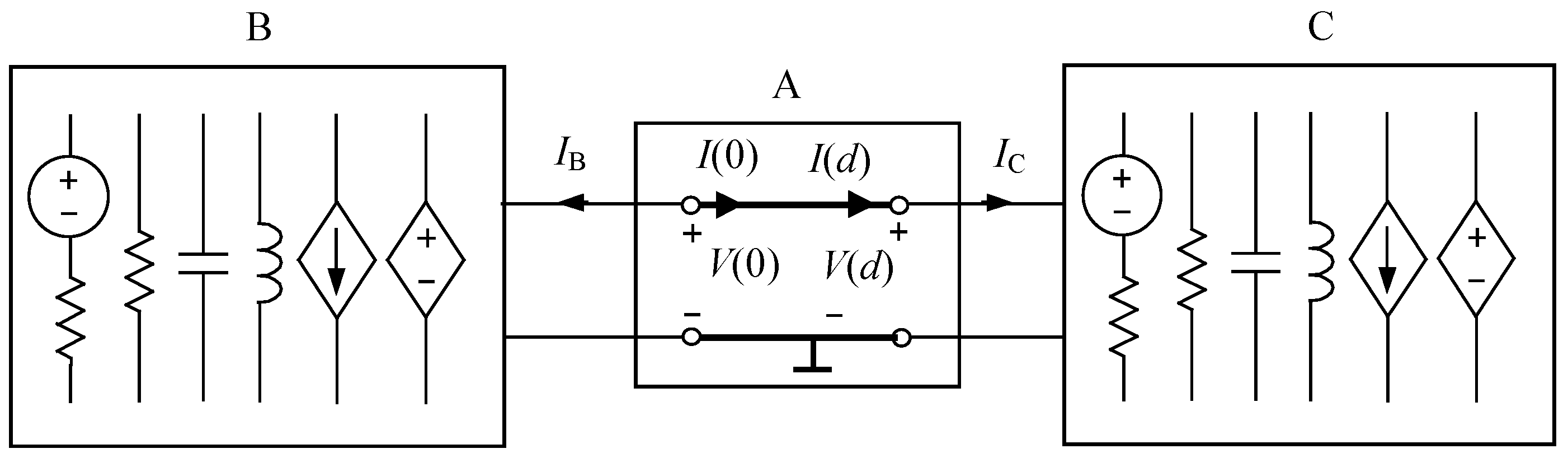
In this paper, we consider linear analog circuits of very high frequency consisting of cascade-connected Blocks A, B, and C, as shown in Figure 1. Block A includes a uniform two-conductor DPTL immersed in a homogenous medium. It has the length d and is specified by the per-unit-length (p-u-l) parameters [23]. Blocks B and C are lumped one-ports, which may contain linear resistors, inductors, capacitors, controlled sources, and independent AC sources. Our goal is to develop a method for parametric fault diagnosis of this class of circuits. The scope of the diagnosis and the main assumptions are as follows.

Assume that only one block, A, B, or C, can be faulty. A parametric fault of the DPTL in Block A, considered in this paper, can be caused by, e.g., the change of geometric dimensions (e.g., the distance between the conductors and their radii), a change of a relative dielectric constant, or a change of electrical resistivity. Thus, the defect occurs along the entire line and has a global nature. It influences the p-u-l parameters of the line. The deviations of these parameters from the nominal values evaluate the fault, and all of them should be determined in the course of the diagnostic process. In Block B or C, only one element may be faulty. Diagnosis of these blocks includes the location of the faulty element and the estimation of its value.

This paper is organized as follows. The basic methodology of the proposed approach is described in Section 2. Section 3 presents an iterative method utilized by the diagnostic method. Three examples and a discussion of the obtained results are demonstrated in Section 4. Section 5 concludes the paper.

2. Parametric Fault Diagnosis Method

To diagnose a circuit belonging to the class defined in Section 1, a measurement test is arranged in the AC state. The phasors $V\left(0\right)$ and $V\left(d\right)$ of the input and output voltages of the DPTL are measured at one frequency while running the test.

2.1. Detection of the Faulty Block

The preliminary step of fault diagnosis is to detect the faulty block or to state that the circuit is fault-free. For this purpose, each of the blocks with nominal parameters is considered separately. In the cases of Blocks B and C, the currents $I_{\mathrm{B}}$ and $I_{\mathrm{C}}$ are determined by the analysis of the blocks driven by the voltage sources $V\left(0\right)$ and $V\left(d\right)$, respectively. The obtained phasors of these currents are denoted by ${\tilde{I}}_{\mathrm{B}}$ and ${\tilde{I}}_{\mathrm{C}}$. Since $V\left(0\right)$ and $V\left(d\right)$ have been measured in the real circuit, which can be faulty, ${\tilde{I}}_{\mathrm{B}}$ or ${\tilde{I}}_{\mathrm{C}}$ is the actual current in the circuit if the corresponding Block B or C is fault-free. Next, we consider Block A including the DPTL driven at the left end by $V\left(0\right)$ and at the right end by $V\left(d\right)$. The line is described by the system of equations:

$$\begin{array}{c}V\left(0\right)-\left(\cosh \gamma d\right)V\left(d\right)-Z_{\mathrm{C}}\left(\sinh \gamma d\right)I\left(d\right)=0\hfill \\ I\left(0\right)-\frac{1}{Z_{\mathrm{C}}}\left(\sinh \gamma d\right)V\left(d\right)-\left(\cosh \gamma d\right)I\left(d\right)=0\hfill \end{array}$$

(1)

where $\gamma =\sqrt{\left(r+\mathrm{j}\omega l\right)\left(g+\mathrm{j}\omega c\right)}$, with $\mathrm{Re}\gamma \ge 0$, $\mathrm{Im}\gamma >0$, is the propagation constant, $Z_{\mathrm{C}}=\sqrt{\frac{r+\mathrm{j}\omega l}{g+\mathrm{j}\omega c}}$, with $\mathrm{Re}{Z}_{\mathrm{C}}\ge 0$, is the characteristic impedance, and the p-u-l parameters, r, l, g, c have nominal values. We solve (1) for $I\left(0\right)$ and $I\left(d\right)$ and denote the solutions by $\tilde{I}\left(0\right)$ and $\tilde{I}\left(d\right)$. They are the actual currents in the circuit if the DPTL is fault-free.

The fault detection and identification of the faulty block is based on

Table 1. Results leading to a set of rules for detecting a faulty block.

Faulty Block	Fault-Free Blocks	Equalities of the Actual and Calculated Currents	Inequalities of the Actual and Calculated Currents	Relationships between the Calculated Currents
no	A, B, C	$I\left(0\right)=\tilde{I}\left(0\right)$, $I\left(d\right)=\tilde{I}\left(d\right)$ $I_{\mathrm{B}}={\tilde{I}}_{\mathrm{B}}$, $I_{\mathrm{C}}={\tilde{I}}_{\mathrm{C}}$	no	${\tilde{I}}_B=-\tilde{I}\left(0\right)$ ${\tilde{I}}_{\mathrm{C}}=\tilde{I}\left(d\right)$
A	B, C	$I_{\mathrm{B}}={\tilde{I}}_{\mathrm{B}}$, $I_{\mathrm{C}}={\tilde{I}}_{\mathrm{C}}$	$I\left(0\right)\ne \tilde{I}\left(0\right)$ $I\left(d\right)\ne \tilde{I}\left(d\right)$	${\tilde{I}}_B\ne -\tilde{I}\left(0\right)$ ${\tilde{I}}_{\mathrm{C}}\ne \tilde{I}\left(d\right)$
B	A, C	$I\left(0\right)=\tilde{I}\left(0\right)$, $I\left(d\right)=\tilde{I}\left(d\right)$ $I_{\mathrm{C}}={\tilde{I}}_{\mathrm{C}}$	$I_{\mathrm{B}}\ne {\tilde{I}}_{\mathrm{B}}$	${\tilde{I}}_B\ne -\tilde{I}\left(0\right)$ ${\tilde{I}}_{\mathrm{C}}=\tilde{I}\left(d\right)$
C	A, B	$I\left(0\right)=\tilde{I}\left(0\right)$, $I\left(d\right)=\tilde{I}\left(d\right)$ $I_{\mathrm{B}}={\tilde{I}}_{\mathrm{B}}$	$I_{\mathrm{C}}\ne {\tilde{I}}_{\mathrm{C}}$	${\tilde{I}}_B=-\tilde{I}\left(0\right)$ ${\tilde{I}}_{\mathrm{C}}\ne \tilde{I}\left(d\right)$

, where $I\left(0\right)$, $I\left(d\right)$, $I_{\mathrm{B}}$, and $I_{\mathrm{C}}$ denote the actual currents in the circuit. The table is created on the assumption, made in Section 1, that only one block, A, B, or C, can be faulty.

The results presented in Table 1 can be summarized as follows.

If ${\tilde{I}}_B=-\tilde{I}\left(0\right)$, ${\tilde{I}}_{\mathrm{C}}=\tilde{I}\left(d\right)$, then the circuit is fault-free.

If ${\tilde{I}}_B\ne -\tilde{I}\left(0\right)$, ${\tilde{I}}_{\mathrm{C}}\ne \tilde{I}\left(d\right)$, then Block A is faulty.

If ${\tilde{I}}_B\ne -\tilde{I}\left(0\right)$, ${\tilde{I}}_{\mathrm{C}}=\tilde{I}\left(d\right)$, then Block B is faulty.

If ${\tilde{I}}_B=-\tilde{I}\left(0\right)$, ${\tilde{I}}_{\mathrm{C}}\ne \tilde{I}\left(d\right)$, then Block C is faulty.

2.2. Diagnosis of the Faulty Block A

If Block A has been detected as faulty (${\tilde{I}}_B\ne -\tilde{I}\left(0\right)$, ${\tilde{I}}_{\mathrm{C}}\ne \tilde{I}\left(d\right)$), we find its actual p-u-l parameters using the two-step procedure.

2.2.1. Step 1

Let us substitute $I\left(0\right)=-{\tilde{I}}_{\mathrm{B}}$, $I\left(d\right)={\tilde{I}}_{\mathrm{C}}$ and the measurement voltages $V\left(0\right)$, $V\left(d\right)$ in (1) and express $\gamma$ and $Z_{\mathrm{C}}$ in the rectangular form: $\gamma =\alpha +\mathrm{j}\beta$, $Z_{\mathrm{C}}=R_{\mathrm{C}}+\mathrm{j}{X}_{\mathrm{C}}$. As a result, we obtain a system of two nonlinear complex equations in four real unknown variables: $\alpha$, $\beta$, $R_{\mathrm{C}}$, $X_{\mathrm{C}}$. This system has the form $\mathbf{g}\left(\mathbf{x}\right)=\mathbf{0}$, where $\mathbf{x}={\left[\alpha \beta R_{\mathrm{C}}{X}_{\mathrm{C}}\right]}^{\mathrm{T}}$, $\mathbf{g}\left(\mathbf{x}\right)={\left[g_1\left(\mathbf{x}\right)g_2\left(\mathbf{x}\right)\right]}^{\mathrm{T}}$, and T denotes transposition. It is solved using the iterative method described in Section 3, where two iteration Formulas (8) and (9) are presented. In the discussed case, each of them consists of four individual real linear equations in four unknown real variables. If (8) generates the sequence that is not convergent, the modified iteration Formula (9) is applied.

2.2.2. Step 2

Having $\alpha$, $\beta$, $R_{\mathrm{C}}$, and $X_{\mathrm{C}}$, the p-u-l parameters of the DPTL are determined as follows. On the basis of equations $\gamma =\alpha +\mathrm{j}\beta$ and $\gamma =\sqrt{\left(r+\mathrm{j}\omega l\right)\left(g+\mathrm{j}\omega c\right)}$, we write:

$$\begin{array}{c}{\gamma }^2={\alpha }^2-{\beta }^2+\mathrm{j}2\alpha \beta \hfill \\ {\gamma }^2= \left(rg-{\omega }^{2}lc\right) + \mathrm{j}\left(\omega lg+\omega rc\right).\hfill \end{array}$$

(2)

Hence, we arrive at two real equations with four real variables r, l, g, and c:

$$\begin{array}{c}rg-{\omega }^{2}lc-{\alpha }^2+{\beta }^2=0\\ \omega lg+\omega rc-2\alpha \beta =0.\end{array}$$

(3)

Similarly, using $Z_{\mathrm{C}}=R_{\mathrm{C}}+\mathrm{j}{X}_{\mathrm{C}}$ and $Z_{\mathrm{C}}=\sqrt{\frac{r+\mathrm{j}\omega l}{g+\mathrm{j}\omega c}}$ gives the equality:

$$R_{\mathrm{C}}^2-X_{\mathrm{C}}^2+\mathrm{j}2R_{\mathrm{C}}{X}_{\mathrm{C}}=\frac{r+\mathrm{j}\omega l}{g+\mathrm{j}\omega c}$$

(4)

leading to two other real equations in four real variables r, l, g, and c:

$$\begin{array}{c}r-\left(R_{\mathrm{C}}^2-X_{\mathrm{C}}^2\right)g+2\omega c{R}_{\mathrm{C}}{X}_{\mathrm{C}}=0\\ \omega l-\omega c\left(R_{\mathrm{C}}^2-X_{\mathrm{C}}^2\right) - 2g{R}_{\mathrm{C}}{X}_{\mathrm{C}}=0.\end{array}$$

(5)

In the systems of Equations (3) and (5), the unknown variables are the p-u-l parameters, r, l, g, and c. Since they have orders that differ significantly one from the other, we scale them using the factors $s_1=1$, $s_2={10}^{-4}$, $s_3={10}^{-7}$, and $s_4={10}^{-11}$. Combining (3) and (5) and substituting $r=s_1{x}_1$, $g=s_2{x}_2$, $l=s_3{x}_3$, and $c=s_4{x}_4$ yield:

$$\begin{array}{c}{s}_1{s}_2{x}_1{x}_2-{\omega }^2{s}_3{s}_4{x}_3{x}_4-{\alpha }^2+{\beta }^2=0\\ \omega s_2{s}_3{x}_2{x}_3+\omega s_1{s}_4{x}_1{x}_4-2\alpha \beta =0\\ s_1{x}_1-\left(R_{\mathrm{C}}^2-X_{\mathrm{C}}^2\right)s_2{x}_2+2\omega R_{\mathrm{C}}{X}_{\mathrm{C}}{s}_4{x}_4=0\\ \omega s_3{x}_3+\omega \left(R_{\mathrm{C}}^2-X_{\mathrm{C}}^2\right)s_4{x}_4-2R_{\mathrm{C}}{X}_{\mathrm{C}}{s}_2{x}_2=0.\end{array}$$

(6)

Let us denote (6) by $\mathbf{g}\left(\mathbf{x}\right)=\mathbf{0}$, where $\mathbf{g}\left(\mathbf{x}\right)={\left[g_1\left(\mathbf{x}\right)\dots g_4\left(\mathbf{x}\right)\right]}^{\mathrm{T}}$, $\mathbf{x}={\left[x_1\dots x_4\right]}^{\mathrm{T}}$ and solve it using the iterative method described in Section 3. Since $\mathbf{g}\left(\mathbf{x}\right)$ is a real function, $\mathbf{D}\left(\mathbf{x}\right)$ is a real $4\times 4$ matrix and $\mathbf{B}\left({\mathbf{x}}^{\left(k\right)}\right)=\mathbf{D}\left({\mathbf{x}}^{\left(k\right)}\right)$. We apply the iteration formula (8), which in this case represents a system of four real linear equations in four unknown real variables. If the generated sequence does not converge, the modified iteration formula (9) is used.

2.3. Diagnosis of the Faulty Block B

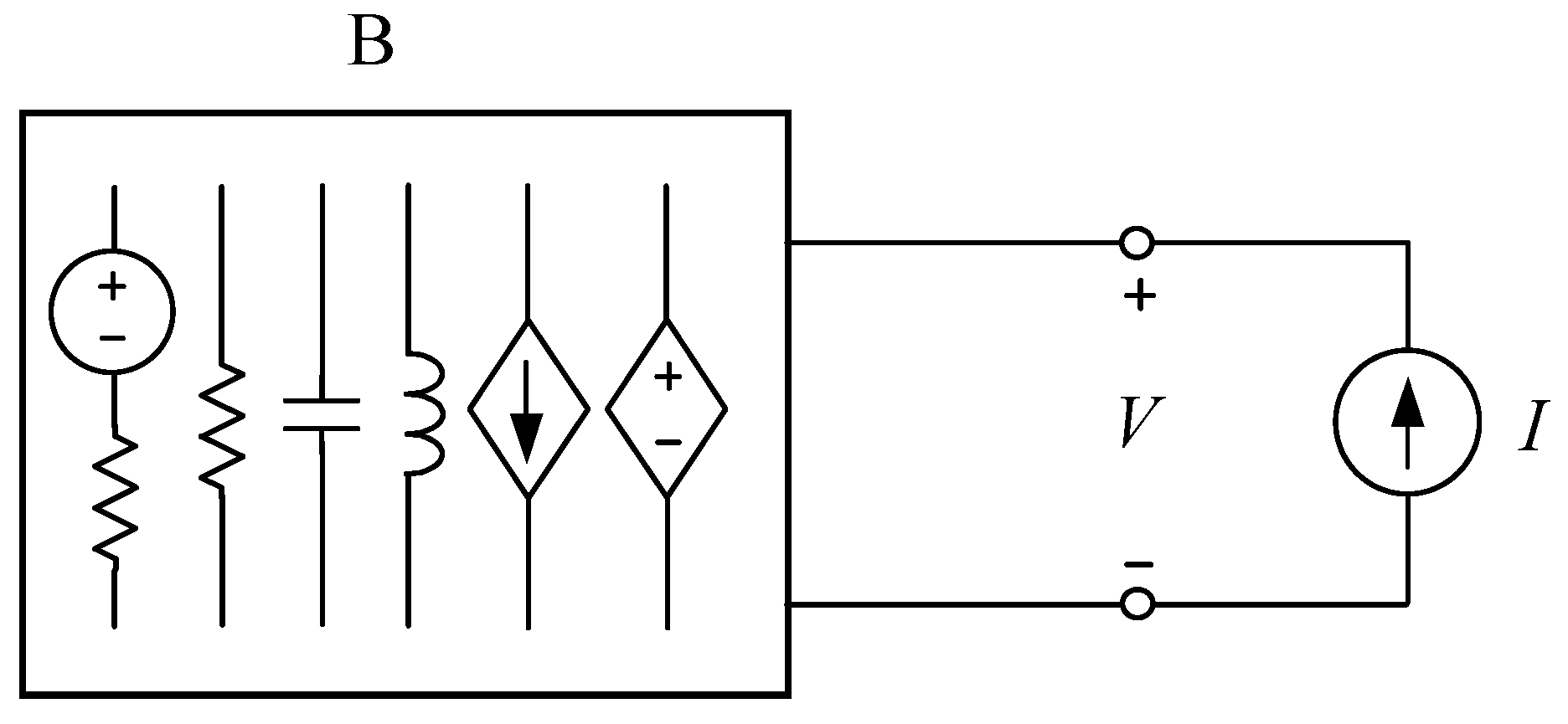
If the preliminary step of the diagnosis states that Block B is faulty (${\tilde{I}}_B\ne -\tilde{I}\left(0\right)$, ${\tilde{I}}_{\mathrm{C}}=\tilde{I}\left(d\right)$), then, according to the assumption made in Section 1, one of the elements of this block is faulty. We wish to locate this element and estimate its value. For this purpose, we consider Block B driven by the current source $I=-\tilde{I}\left(0\right)$, as shown in Figure 2.

Since the input voltage V is equal to the measured voltage $V\left(0\right)$, both I and V are given. Let us describe the circuit depicted in Figure 2 using the node method, leading to a system of N complex equations. Because V is one of the node voltages, the number of unknown variables is $N-1$. We present them in rectangular form obtaining $2N-2$ real variables. Let us increase the number of variables to $2N-1$ by adding one of the circuit parameters considered as potentially faulty. As a result, we obtain a system of N complex equations in $2N-1$ real variables, which can be presented in the compact form $\mathbf{g}\left(\mathbf{x}\right)=\mathbf{0}$. To solve them, we apply the method described in Section 3 where $n=N$, $m=2N-1$ and $\mathbf{B}\left({\mathbf{x}}^{\left(k\right)}\right)$ is a $2N\times \left(2N-1\right)$ matrix. The iteration Formula (8) consists of $2N-1$ real equations in $2N-1$ real unknown variables. They include $2N-2$ real and imaginary parts of the node voltage phasors and one unknown parameter, whereas the other parameters have nominal values. If the method based on the iteration Formula (8) does not converge, the modified Formula (9) is used. We repeat this approach for each of the parameters in Block B considered as potentially faulty. Every time, the solution includes one unknown parameter and $2N-2$ redundant real variables. When the chosen parameter is faulty, we obtain the correct result. Otherwise, the method can give non-realistic solutions or not be convergent. Sometimes, the method may find a virtual solution.

Note 1. If Block B contains elements not acceptable by the node method, the modified node method is applied.

Note 2. Diagnosis of Block C is carried out analogously.

3. Solving a System of Nonlinear Algebraic Equations

3.1. Standard Method

Let us consider a system of n nonlinear complex equations in m unknown real variables presented in a compact form:

$$\mathbf{g}\left(\mathbf{x}\right)=\mathbf{0}$$

(7)

where $\mathbf{x}={\left[x_1\cdots x_m\right]}^{\mathrm{T}}$, $\mathbf{g}\left(\mathbf{x}\right)={\left[g_1\left(\mathbf{x}\right)\cdots g_n\left(\mathbf{x}\right)\right]}^{\mathrm{T}}$, $2n\ge m$. To solve this equation, the iterative method developed in [24] can be used. This iteration formula:

$${\mathbf{B}}^{\mathrm{T}}\left({\mathbf{x}}^{\left(k\right)}\right)\mathbf{B}\left({\mathbf{x}}^{\left(k\right)}\right)\left({\mathbf{x}}^{\left(k+1\right)}-{\mathbf{x}}^{\left(k\right)}\right)=\mathbf{b}\left({\mathbf{x}}^{\left(k\right)}\right)$$

(8)

represents a system of m real individual linear equations in m real unknowns $x_1^{\left(k+1\right)}$, …, $x_m^{\left(k+1\right)}$ at $k=0,1,2,\dots$, where k is the index of iteration:

$$\mathbf{B}\left({\mathbf{x}}^{\left(k\right)}\right)=\left[\begin{array}{c}\mathrm{Re}\mathbf{D}\left({\mathbf{x}}^{\left(k\right)}\right)\\ \mathrm{Im}\mathbf{D}\left({\mathbf{x}}^{\left(k\right)}\right)\end{array}\right],$$

$$\mathbf{b}\left({\mathbf{x}}^{\left(k\right)}\right)=-{\mathbf{B}}^{\mathrm{T}}\left({\mathbf{x}}^{\left(k\right)}\right)\left[\begin{array}{c}\mathrm{Re}\mathbf{g}\left({\mathbf{x}}^{\left(k\right)}\right)\\ \mathrm{Im}\mathbf{g}\left({\mathbf{x}}^{\left(k\right)}\right)\end{array}\right]$$

where:

$$\mathbf{D}\left({\mathbf{x}}^{\left(k\right)}\right)=\left[\begin{array}{ccc}{\displaystyle \frac{\partial g_1}{\partial x_1}}\left({\mathbf{x}}^{\left(k\right)}\right)& \cdots & {\displaystyle \frac{\partial g_1}{\partial x_m}}\left({\mathbf{x}}^{\left(k\right)}\right)\\ \cdots \cdots \cdots & \cdots & \cdots \cdots \cdots \\ {\displaystyle \frac{\partial g_n}{\partial x_1}}\left({\mathbf{x}}^{\left(k\right)}\right)& \cdots & {\displaystyle \frac{\partial g_n}{\partial x_m}}\left({\mathbf{x}}^{\left(k\right)}\right)\end{array}\right].$$

Matrix $\mathbf{B}\left({\mathbf{x}}^{\left(k\right)}\right)$ has order $2n\times m$; matrix $\mathbf{D}\left({\mathbf{x}}^{\left(k\right)}\right)$ has order $n\times m$; and $\mathbf{b}\left({\mathbf{x}}^{\left(k\right)}\right)$ is an $m\times 1$ vector. As a consequence, ${\mathbf{B}}^{\mathrm{T}}\left({\mathbf{x}}^{\left(k\right)}\right)\mathbf{B}\left({\mathbf{x}}^{\left(k\right)}\right)$ is a real square matrix of order $m\times m$. If the iteration process specified by (8) converges, it is terminated when $\underset{1\le i\le m}{\max }\frac{\left|x_i^{\left(k+1\right)}-x_i^{\left(k\right)}\right|}{{\left|x_i^{\left(k\right)}\right|}^{}}<{\epsilon }_x$ and $\underset{1\le i\le n}{\max }\left|g_i\left({\mathbf{x}}^{\left(k+1\right)}\right)\right|<{\epsilon }_f$, where ${\epsilon }_x$ and ${\epsilon }_f$ are convergence tolerances, and ${\mathbf{x}}^{\left(k+1\right)}$ is considered as an approximate solution. If the method does not meet the convergence tolerances in a preset maximum number of iterations $M_{\mathrm{it}}$, it fails.

3.2. Modified Method

The difficulty of solving (7) arises if the standard method does not converge. In such a case, we modify it as described in the sequel.

The $m\times m$ matrix ${\mathbf{B}}^{\mathrm{T}}\left({\mathbf{x}}^{\left(k\right)}\right)\mathbf{B}\left({\mathbf{x}}^{\left(k\right)}\right)$ is symmetrical for each $k=0,1,\dots$, because ${\left[{\mathbf{B}}^{\mathrm{T}}\left({\mathbf{x}}^{\left(k\right)}\right)\mathbf{B}\left({\mathbf{x}}^{\left(k\right)}\right)\right]}^{\mathrm{T}}={\mathbf{B}}^{\mathrm{T}}\left({\mathbf{x}}^{\left(k\right)}\right)\mathbf{B}\left({\mathbf{x}}^{\left(k\right)}\right)$ and positive semidefinite because for any real $m\times 1$ vector $\mathbf{y}$: ${\mathbf{y}}^{\mathrm{T}}\left[{\mathbf{B}}^{\mathrm{T}}\left({\mathbf{x}}^{\left(k\right)}\right)\mathbf{B}\left({\mathbf{x}}^{\left(k\right)}\right)\right]\mathbf{y}={\left[\mathbf{B}\left({\mathbf{x}}^{\left(k\right)}\right)\mathbf{y}\right]}^{\mathrm{T}}\mathbf{B}\left({\mathbf{x}}^{\left(k\right)}\right)\mathbf{y}\ge 0$. Thus, its determinant is greater than or equal to zero. When $\det \left[{\mathbf{B}}^{\mathrm{T}}\left({\mathbf{x}}^{\left(k\right)}\right)\mathbf{B}\left({\mathbf{x}}^{\left(k\right)}\right)\right]=0$, the iterative method fails. Even if the determinant is close to zero, the method may not converge. To get rid of this drawback, we propose a new iteration formula as follows:

$${\left[{\mathbf{B}}^{\mathrm{T}}\left({\mathbf{x}}^{\left(k\right)}\right)\mathbf{B}\left({\mathbf{x}}^{\left(k\right)}\right)+\xi {\mathrm{e}}^{-\mu k}\mathbf{1}\right]}^{}\left({\mathbf{x}}^{\left(k+1\right)}-{\mathbf{x}}^{\left(k\right)}\right)=\mathbf{b}\left({\mathbf{x}}^{\left(k\right)}\right)$$

(9)

where $\xi$ and $\mu$ are positive constants selected based on numerical experiments. Since $\xi {\mathrm{e}}^{-\mu k}\mathbf{1}$ is a diagonal matrix with identical positive elements $\xi {\mathrm{e}}^{-\mu k}$ on the main diagonal, the matrix $\left[{\mathbf{B}}^{\mathrm{T}}\left({\mathbf{x}}^{\left(k\right)}\right)\mathbf{B}\left({\mathbf{x}}^{\left(k\right)}\right)+\xi {\mathrm{e}}^{-\mu k}\mathbf{1}\right]$ is positive definite for all $k=1,2,\dots$, because for any real $m\times 1$ vector $\mathbf{y}\ne \mathbf{0}$:

${\mathbf{y}}^{\mathrm{T}}\left[{\mathbf{B}}^{\mathrm{T}}\left({\mathbf{x}}^{\left(k\right)}\right)\mathbf{B}\left({\mathbf{x}}^{\left(k\right)}\right)+\xi {\mathrm{e}}^{-\mu k}\mathbf{1}\right]\mathbf{y}$ = ${\left[\mathbf{B}\left({\mathbf{x}}^{\left(k\right)}\right)\mathbf{y}\right]}^{\mathrm{T}}\mathbf{B}\left({\mathbf{x}}^{\left(k\right)}\right)\mathbf{y}+\xi {\mathrm{e}}^{-\mu k}{\mathbf{y}}^{\mathrm{T}}\mathbf{y}>0$.

Then, its determinant is greater than zero, and Equation (9) can be uniquely solved at any iteration. As k increases, the diagonal elements of the matrix $\xi {\mathrm{e}}^{-\mu k}\mathbf{1}$ decrease and tend to zero for large values of k. As a consequence, Equation (9) approaches Equation (8).

4. Illustrative Examples

The diagnostic method proposed in Section 2 and Section 3 was implemented in the MATLAB environment, and the calculations were performed on a PC with an Intel Core i7-6700 processor. To show the efficiency of the method, three numerical examples are presented. Whenever the iterative method described in Section 3 is employed, the nominal values of the fault-free variables are chosen to form the initial guess.

4.1. Example 1

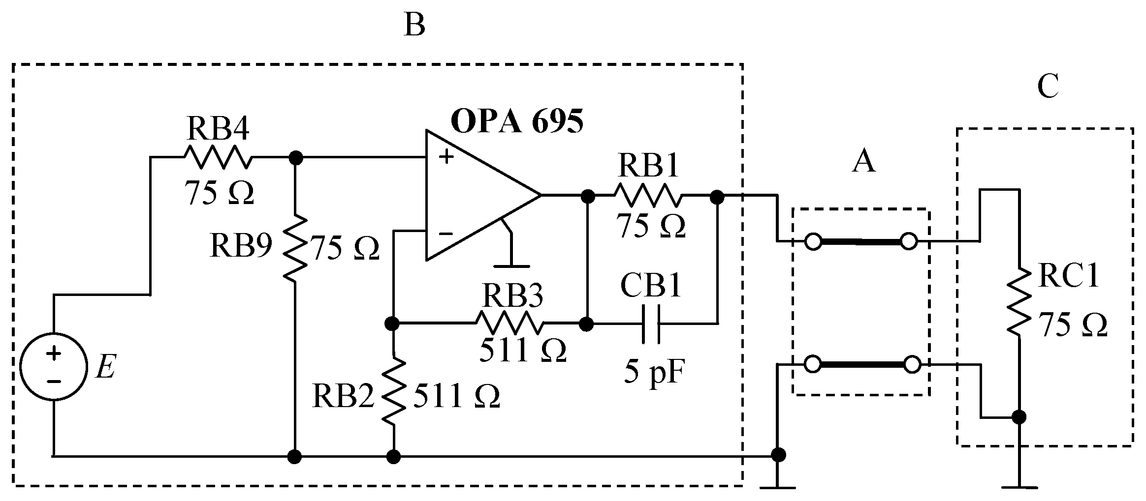
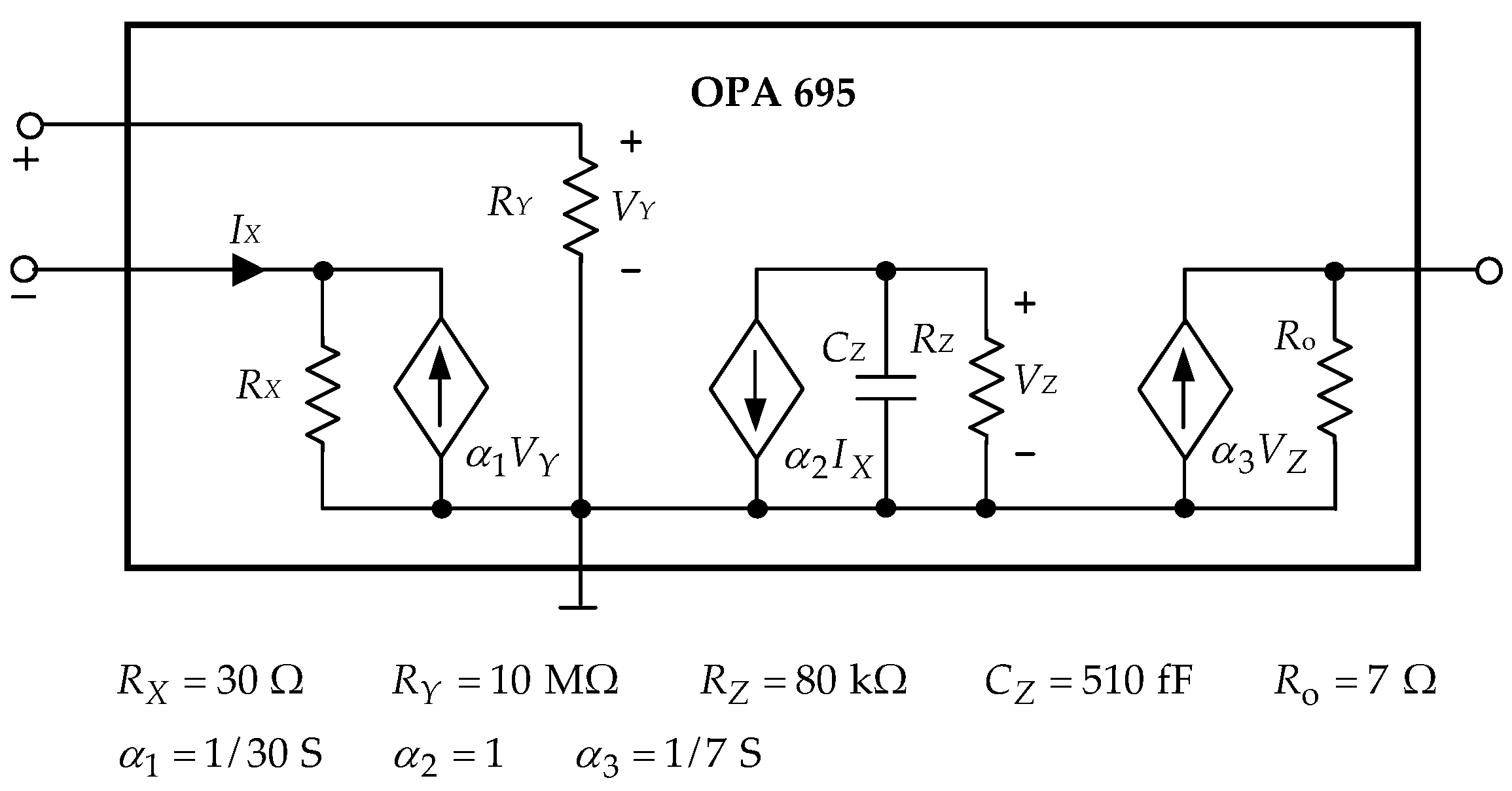
Figure 3 shows a basic wideband impedance-matched line driver, configured to drive a coaxial cable RG59 and 75 load. It includes the current-feedback operational amplifier, two-conductor DPTL, and lumped elements. The model OPA 695 used in the simulations is depicted in Figure 4. For this model, very good compatibility of the frequency responses in the frequency range 100 Hz–200 MHz and the time responses was achieved compared to the full model available in the IsSPICE software.

The nominal values of the lumped elements existing in the circuit and in the OPA 695 model are indicated in Figure 3 and Figure 4, whereas the nominal p-u-l parameters of the DPTL are as follows: $r=1.6442\mathsf{\Omega }/\mathrm{m}$, $g=2.0050\times {10}^{-4}\mathrm{S}/\mathrm{m}$, $l=3.6978\times {10}^{-7}\mathrm{H}/\mathrm{m}$, $c=6.7608\times {10}^{-11}\mathrm{F}/\mathrm{m}$, and the length d of the line is 1 m. The amplitude of the voltage source E is 2 V, and the phase is $0^{\circ }$, $f=100\mathrm{MHz}$. The accuracy of the measurements of the voltage amplitudes is $0.1\mathrm{mV}$ and of the phase $0.{01}^{\circ }$. The convergence tolerances and constants are: ${\epsilon }_x=1\times {10}^{-6}$, ${\epsilon }_f=1\times {10}^{-5}$, $M_{\mathrm{it}}=100$, $\xi ={10}^{-5}$, $\mu =1$.

In the circuit of Figure 3, we diagnosed 5 faults of Block A, 17 faults of Block B, and 3 faults of Block C. In all these cases, the procedure for detecting the faulty block, described in Section 2.1, gave the correct outcomes.

The findings of the diagnoses of five faults of Block A are placed in

Table 2. Results of the diagnosis of faulty Block A including the DPTL.

	$\mathit{r}(\mathsf{\Omega }/\mathbf{m})$	$\mathit{l}(\mathbf{H}/\mathbf{m})\times {10}^7$	$\mathit{g}(\mathbf{S}/\mathbf{m})\times {10}^4$	$\mathit{c}(\mathbf{F}/\mathbf{m})\times {10}^{11}$
Nominal values	1.6442	3.6978	2.0050	6.7608
1. Actual values	1.2609	3.3834	2.1914	9.3596
Values given by the method	1.2666	3.3826	2.1778	9.3618
2. Actual values	2.1091	4.2640	1.7388	6.6447
Values given by the method	2.0922	4.2627	1.7736	6.6468
3. Actual values	1.5199	3.5146	2.1095	7.4292
Values given by the method	1.3391	3.5165	2.4826	7.4252
4. Actual values	1.3485	3.2786	2.2614	8.4725
Values given by the method	1.3578	3.2787	2.2524	8.4721
5. Actual values	1.4035	3.3834	2.1914	9.3596
Values given by the method	1.4251	3.3833	2.1303	9.3601

. Every time, all the p-u-l parameters of the line are calculated. The relative error:

$${\epsilon }_{\mathrm{r}}=\frac{\left|x^{\mathrm{actual}}-x^{\mathrm{calculated}}\right|}{x^{\mathrm{actual}}}100\%$$

(10)

of the 20 parameter values presented in this table is as follows. In 15 cases $\left(75\%\right)$, ${\epsilon }_{\mathrm{r}}<1\%$; in three cases $\left(15\%\right)$, $1\%<{\epsilon }_{\mathrm{r}}<3\%$; in two cases, (10%), $10\%<{\epsilon }_{\mathrm{r}}<18\%$. To obtain the results summarized in Table 2, the iterative method, based on the iteration Formula (8), was used. The number of iterations for finding $\alpha$, $\beta$, $R_{\mathrm{C}}$, and $X_{\mathrm{C}}$ (Step 1) ranges from six to 22 and for finding the p-u-l parameters (Step 2) is four in all the cases.

Table 3. Results of the diagnosis of faulty Block B for different values of the defective resistor RB1 whose nominal value is 75 $\mathsf{\Omega }$.

Number of the Fault	1	2	3	4	5
Actual value of RB1 in $\mathsf{\Omega }$	1	15	55	90	250
Value of RB1 in $\mathsf{\Omega }$ given by the method	1.0057	14.9997	54.9346	89.7956	248.3287

,

Table 4. Results of the diagnosis of faulty Block B for different values of the defective resistor RB2 whose nominal value is 511 $\mathsf{\Omega }$.

Number of the Fault	1	2	3	4
Actual value of RB2 in $\mathsf{\Omega }$	300	450	670	1500
Value of RB2 in $\mathsf{\Omega }$ given by the method	300.1964	450.8073	669.5704	1499.6

,

Table 5. Results of the diagnosis of faulty Block B for different values of the defective resistor RB3 whose nominal value is 511 $\mathsf{\Omega }$.

Number of the Fault	1	2	3	4
Actual value of RB3 in $\mathsf{\Omega }$	250	400	620	1000
Value of RB3 in $\mathsf{\Omega }$ given by the method	251.5692	400.1235	618.0379	1000.9

and

Table 6. Results of the diagnosis of faulty Block B for different values of the defective capacitor CB1 whose nominal value is 5 pF.

Number of the Fault	1	2	3	4
Actual value of CB1 in pF	1	4	6	50
Value of CB1 in pF given by the method	1.0227	4.0245	6.0290	49.9900

present 17 cases of the faults of Block B caused by 5 faults of the resistor RB1 (Table 3), 4 faults of the resistor RB2 (Table 4), 4 faults of the resistor RB3 (Table 5), and 4 faults of the capacitor CB1 (Table 6).

The outcomes summarized in Table 3 are quite accurate; ${\epsilon }_{\mathrm{r}}$ does not exceed 0.7%. To diagnose Faults 1 and 2, the proposed iteration Formula (9) was used because the sequences generated by the iteration Formula (8) were not convergent. In the case of Fault 4, the method finds correctly the faulty resistor $\mathrm{RB}1=89.7956\mathsf{\Omega }$, inserted in the table, and a virtual fault $\mathrm{RB}3=421.7773\mathsf{\Omega }$. The number of iterations needed to determine each parameter value presented in the table varies from five to 13, and the CPU time does not exceed 0.33 s.

The findings inserted in Table 4 are very accurate; ${\epsilon }_{\mathrm{r}}$ is smaller than 0.18%. The number of iterations ranges from five to eight, and the CPU time does not exceed 0.32 s.

The relative error ${\epsilon }_{\mathrm{r}}$ of the resistor values posted in Table 5 is less than 0.7%; the number of iterations varies from five to six; and the CPU time does not exceed 0.36 s. In the cases of Faults 2 and 3 placed in this table, the method gives the correct faulty resistors and virtual ones. The virtual fault is $\mathrm{RB}1=93.8013\mathsf{\Omega }$ in Case 2 and $\mathrm{RB}1=60.6634\mathsf{\Omega }$ in Case 3. However, if the accuracy of the measurement in the diagnostic test course is increased ($0.01\mathrm{mV}$ for the amplitude and $0.{001}^{\circ }$ for the phase), the method provides only the correct findings. Unfortunately, it is difficult to ensure such high accuracy in real conditions.

The relative error ${\epsilon }_{\mathrm{r}}$ of the outcomes placed in Table 6 is less than 2.8%; the number of iterations ranges from 4–6; and the CPU time does not exceed 0.063 s.

Table 7. Results of the diagnosis of faulty Block C for different values of the defective resistor RC1 whose nominal value is 75 $\mathsf{\Omega }$.

Number of the Fault	1	2	3
Actual value of RC1 in $\mathsf{\Omega }$	55	85	100
Value of RC1 in $\mathsf{\Omega }$ given by the method	54.9579	85.0143	99.7647

contains the results of the diagnosis of the faulty Block C. They were obtained performing 4–5 iterations and are burdened with very small relative error, ${\epsilon }_{\mathrm{r}}<0.2\%$. The CPU time does not exceed 0.095 s.

4.2. Example 2

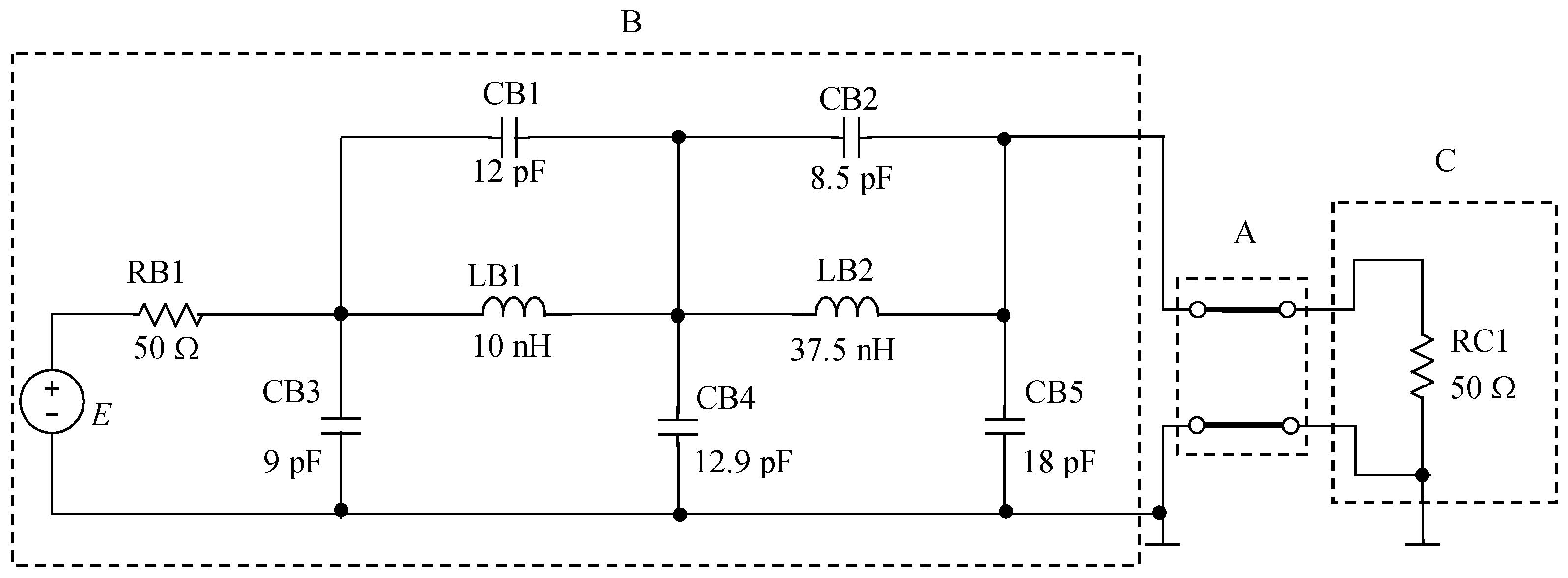
Let us consider the circuit, including the 150 MHz elliptical low-pass filter and the DPTL terminated by a resistor, shown in Figure 5. The nominal values of the lumped elements are indicated in the figure, whereas the nominal p-u-l parameters of the DPTL are as follows: $r=1.3054\mathsf{\Omega }/\mathrm{m}$, $g=2.8681\times {10}^{-4}\mathrm{S}/\mathrm{m}$, $l=2.5851\times {10}^{-7}\mathrm{H}/\mathrm{m}$, $c=9.6710\times {10}^{-11}\mathrm{F}/\mathrm{m}$, and the length d of the line is 0.7 m. The amplitude of the voltage source E is 5 V, and the phase is $0^{\circ }$, $f=100\mathrm{MHz}$. The accuracy of the measurements of the voltage amplitudes is $0.1\mathrm{mV}$ and of the phase $0.{01}^{\circ }$. The convergence tolerances and constants are: ${\epsilon }_x=1\times {10}^{-6}$, ${\epsilon }_f=1\times {10}^{-5}$, $M_{\mathrm{it}}=100$, $\xi ={10}^{-5}$, and $\mu =1$.

We performed 39 diagnoses including 4 faults of Block A, 30 faults of Block B, and 5 faults of Block C. In all cases, the procedure for detecting the faulty block, described in Section 2.1, gave the correct results.

The outcomes of the diagnoses of four faults of Block A are summarized in

Table 8. Results of the diagnosis of faulty Block A including the DPTL.

	$\mathit{r}(\mathsf{\Omega }/\mathbf{m})$	$\mathit{l}(\mathbf{H}/\mathbf{m})\times {10}^7$	$\mathit{g}(\mathbf{S}/\mathbf{m})\times {10}^4$	$\mathit{c}(\mathbf{F}/\mathbf{m})\times {10}^{11}$
Nominal values	1.3054	2.5851	2.8681	9.6710
1. Actual values	1.2649	3.0252	2.4508	9.7331
Values given by the method	1.2518	3.0251	2.5047	9.7338
2. Actual values	1.2612	2.9270	2.5331	8.5413
Values given by the method	1.2698	2.9273	2.5043	8.5409
3. Actual values	1.2975	1.9332	3.8354	18.680
Values given by the method	1.3036	1.9329	3.7608	18.684
4. Actual values	1.0686	1.9524	3.7975	16.220
Values given by the method	1.0751	1.9525	3.7483	16.218

. In 11 cases $\left(68.7\%\right)$, the relative error ${\epsilon }_{\mathrm{r}}$ of the results provided by the method was less than 1%; in the remaining five cases $\left(31.3\%\right)$ it is greater than 1%, but smaller than 2.2%. The number of iterations for finding $\alpha$, $\beta$, $R_{\mathrm{C}}$, and $X_{\mathrm{C}}$ (Step 1) ranges from five to six and for finding the p-u-l parameters (Step 2) from four to five.

In Block B, all the elements can be diagnosed except CB1 and CB2, because the sensitivities of the voltage of this block with respect to these elements are very small. Consequently, for realistic measurement accuracy, variations of these elements have a very small influence on the voltage. All the other elements of this block, RB1, CB3, CB4, CB5, LB1, and LB2, were diagnosed.

Table 9. Results of the diagnosis of faulty Block B for different values of the defective resistor RB1 whose nominal value is 50 $\mathsf{\Omega }$.

Number of the Fault	1	2	3	4	5
Actual value of RB1 in $\mathsf{\Omega }$	10	30	65	75	150
Value of RB1 in $\mathsf{\Omega }$ given by the method	10.0005	29.9986	64.9948	75.0044	150.0111

,

Table 10. Results of the diagnosis of faulty Block B for different values of the defective capacitor CB3 whose nominal value is 9 pF.

Number of the Fault	1	2	3	4	5
Actual value of CB3 in pF	1	5	11.7	15	50
Value of CB3 in pF given by the method	1.0002	5.0024	11.701	14.997	50.001

,

Table 11. Results of the diagnosis of faulty Block B for different values of the defective capacitor CB4 whose nominal value is 12.9 pF.

Number of the Fault	1	2	3	4	5
Actual value of CB4 in pF	3.9	8	9	18	50
Value of CB4 in pF given by the method	3.8969	7.9999	8.9992	18.001	49.998

,

Table 12. Results of the diagnosis of faulty Block B for different values of the defective capacitor CB5 whose nominal value is 18 pF.

Number of the Fault	1	2	3	4	5
Actual value of CB5 in pF	1	10	12.6	22	50
Value of CB5 in pF given by the method	0.9967	10.002	12.602	22.002	49.999

,

Table 13. Results of the diagnosis of faulty Block B for different values of the defective inductor LB1 whose nominal value is 10 nH.

Number of the Fault	1	2	3	4	5
Actual value of LB1 in nH	5	7	15	25	50
Value of LB1 in nH given by the method	Fail	7.002	14.996	24.996	50.003

and

Table 14. Results of the diagnosis of faulty Block B for different values of the defective inductor LB2 whose nominal value is 37.5 nH.

Number of the Fault	1	2	3	4	5
Actual value of LB2 in nH	5	26.3	32	47	80
Value of LB2 in nH given by the method	5.002	26.294	32.001	47.003	79.999

present 30 cases of the faults including five faults of the resistor RB1 and five faults of each of the capacitors CB3, CB4, and CB5 and the inductors LB1 and LB2.

The outcomes placed in Table 9 are very accurate, and ${\epsilon }_{\mathrm{r}}<0.01\%$. The number of iterations ranges from four to six, and the CPU time of each of the diagnoses does not exceed 0.1 s. To diagnose Fault 1, the proposed iteration Formula (9) was used because the sequence generated by the iteration Formula (8) was not convergent.

The findings presented in Table 10 and Table 11 are very accurate (${\epsilon }_{\mathrm{r}}<0.08\%$); the number of iterations varies from four to five, and CPU time does not exceed 0.21 s.

The maximum relative error of the results included in Table 12 is ${\epsilon }_{\mathrm{r}}<0.33\%$, and the number of iterations in all the cases is two. The CPU time is 0.16 s.

The outcomes summarized in Table 13 and Table 14 are very accurate; ${\epsilon }_{\mathrm{r}}<0.04\%$. The number of iterations ranges from four to 14. The CPU time is 0.16 s.

The relative error ${\epsilon }_{\mathrm{r}}$ of the resistor values inserted in

Table 15. Results of the diagnosis of faulty Block C for different values of the defective resistor RC1 whose nominal value is 50 $\mathsf{\Omega }$.

Number of the Fault	1	2	3	4	5
Actual value of RC1 in $\mathsf{\Omega }$	5	35	65	75	100
Value of RC1 in $\mathsf{\Omega }$ given by the method	5.0006	34.999	64.995	74.989	99.999

is less than 0.02%. The number of iterations varies from five to nine. The CPU time is 0.19 s. To diagnose Fault 1, the proposed iteration formula (9) was used because the sequence generated by the iteration formula (8) was not convergent.

4.3. Example 3

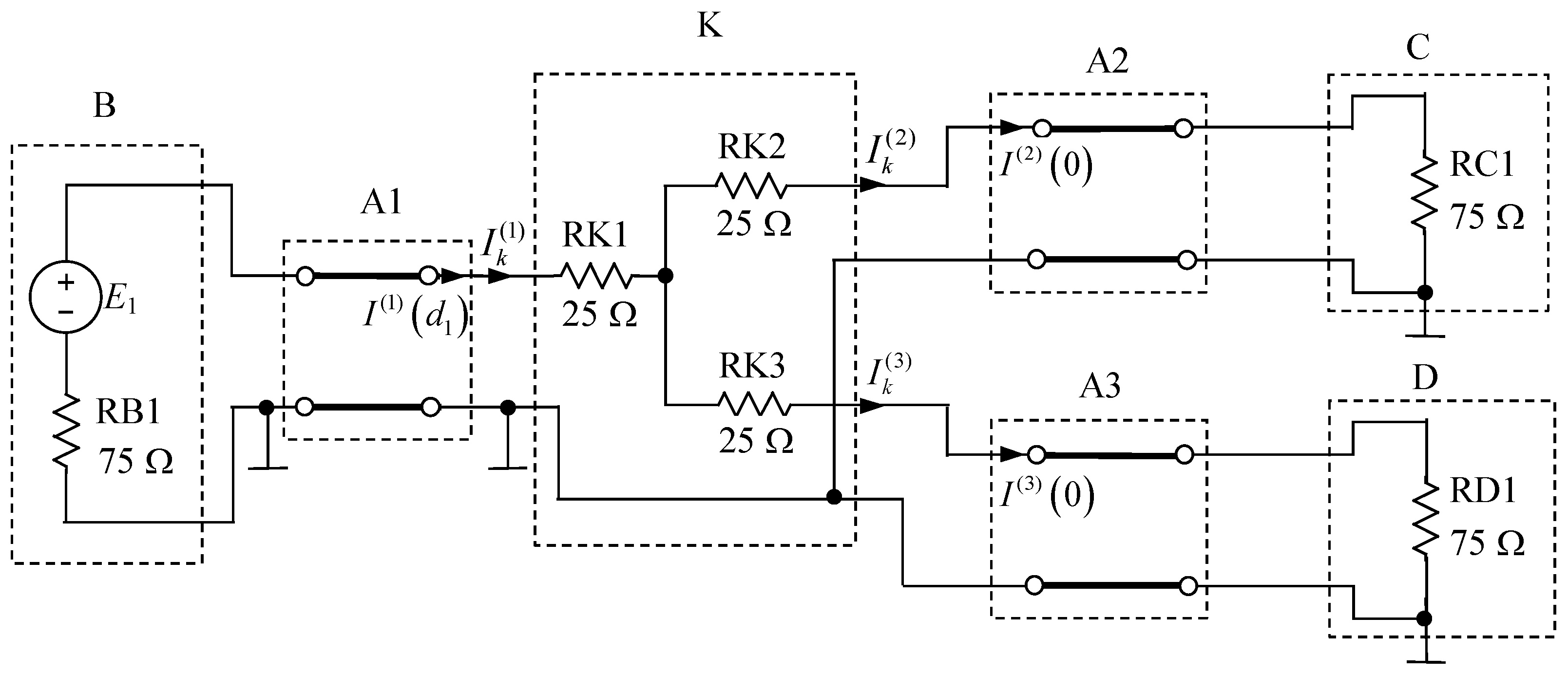
Figure 6 shows the circuit including three DPTLs, A1, A2, and A3, having the p-u-l parameters: $r=1.6442\mathsf{\Omega }/\mathrm{m}$, $g=2.0050\times {10}^{-4}\mathrm{S}/\mathrm{m}$, $l=3.6978\times {10}^{-7}\mathrm{H}/\mathrm{m}$, $c=6.7608\times {10}^{-11}\mathrm{F}/\mathrm{m}$. The lengths of the lines are $d_1=0.7\mathrm{m}$, $d_2=0.5\mathrm{m}$, and $d_3=0.4\mathrm{m}$. The nominal values of the lumped elements are indicated in the figure; the amplitude of the voltage source $E_1$ equals 5 V; and the phase is $0^{\circ }$. The other parameters are as in Example 2.

The circuit of Figure 6 has a more complex structure than that shown in Figure 1. It consists of three blocks, A1, A2, and A3, containing DPTLs and four blocks, B, C, D, and K, including lumped elements. Similarly, as in Section 1, we assume that only one block can be faulty and only one element of the lumped block can be defective. In the blocks containing DPTLs, all the p-u-l parameters may deviate from nominal values due to a fault, and all of them must be diagnosed. The diagnostic test of the circuit requires the input and output voltages of each DPTL. The fault detection rule presented in Section 2.1 for three-block circuits can be directly extended to the circuit of Figure 6. In particular, the three-port Block K is faulty if ${\tilde{I}}_K^{\left(1\right)}\ne {\tilde{I}}^{\left(1\right)}\left(d_1\right)$ , ${\tilde{I}}_K^{\left(2\right)}\ne {\tilde{I}}^{\left(2\right)}\left(0\right)$ ,and ${\tilde{I}}_K^{\left(3\right)}\ne {\tilde{I}}^{\left(3\right)}\left(0\right)$.

In the circuit of Figure 6, we diagnosed three faults of each of Blocks A1, A2, A3, B, C, and D and nine faults of Block K. In all these cases, the procedure for detecting a faulty block gave correct outcomes.

The findings of the diagnoses of six faults of Blocks A1, A2, and A3 (24 parameters) are placed in

Table 16. Results of the diagnosis of faulty Blocks A1, A2, and A3 including DPTLs.

		$\mathit{r}\left(\mathsf{\Omega }/\mathbf{m}\right)$	$\mathit{l}\left(\mathbf{H}/\mathbf{m}\right)\times {10}^7$	$\mathit{g}\left(\mathbf{S}/\mathbf{m}\right)\times {10}^4$	$\mathit{c}\left(\mathbf{F}/\mathbf{m}\right)\times {10}^{11}$
	Nominal values	1.6442	3.6978	2.0050	6.7608
	1. Actual values	1.8767	3.5150	2.1100	7.4290
Line	Values given by the method	1.8762	3.5150	2.1165	7.4289
A1	2. Actual values	1.4444	3.0397	2.4391	7.4035
	Values given by the method	1.4526	3.0395	2.4259	7.4931
	1. Actual values	1.3485	3.2790	2.2610	8.4720
Line	Values given by the method	1.3647	3.2788	2.1980	8.4728
A2	2. Actual values	1.9518	3.2190	2.3030	1.0010
	Values given by the method	1.9371	3.2186	2.3660	1.0010
	1. Actual values	0.9852	3.5120	2.1110	6.4860
Line	Values given by the method	1.0042	3.5119	2.0973	6.4859
A3	2. Actual values	1.8235	3.2190	2.3030	1.1220
	Values given by the method	1.8493	3.2210	2.2196	1.1211

. In 18 cases (75%), ${\epsilon }_{\mathrm{r}}<1\%$, and in six cases (25%), $1\%<{\epsilon }_{\mathrm{r}}<4\%$. The number of iterations in Step 1 ranges from 4–7 and in Step 2 from 4–5.

Table 17. Results of the diagnosis of faulty Blocks B, C, and D for different values of the defective resistors RB1, RC1, and RD1.

	Actual Value in $\mathsf{\Omega }$	Value, in $\mathsf{\Omega }$, Given by the Method
RB1	30	29.999
	55	55.000
RC1	45	45.001
	100	100.001
RD1	50	49.999
	150	150.011

and

Table 18. Results of the diagnosis of faulty Block K for different values of the defective resistors RK1, RK2, and RK3.

	Actual Value in $\mathsf{\Omega }$	Value, in $\mathsf{\Omega }$, Given by the Method
RK1	10	10.000
	75	74.997
RK2	10	10.004
	50	50.005
RK3	2	2.002
	90	90.006

present the results of the diagnoses of two faults in each of Blocks B, C, and D and six faults in Block K. To diagnose Block K, which is a three-port circuit, an obvious modification of the procedure described in Section 2.3 is needed. The results are very accurate; the number of iterations ranges from 5–15; and the CPU time does not exceed 0.4 s. In three cases, corresponding to $\mathrm{RB}1=30\mathsf{\Omega }$, $\mathrm{RK}1=10\mathsf{\Omega }$, and $\mathrm{RK}3=2\mathsf{\Omega }$, the iteration formula (9) was used because the iteration sequences generated by formula (8) were not convergent.

5. Conclusions

Parametric fault diagnosis of analog circuits of very high frequency consisting of a distributed parameter transmission line, as well as lumped linear passive and active elements has not been discussed in the literature till now. This paper deals with the problem and proposes a method that covers all aspects of the fault diagnosis. First, the faulty area is determined, and then, the faulty component inside this area is located and its value estimated. There are three areas in the circuit, called blocks, including the DPTL (Block A) and two lumped circuits terminating the line (Blocks B and C). It is assumed that only one block may be faulty and only one component of the faulty Block B or C can be defective. The blocks may include IC devices if they can be represented by realistic linear models. The example is the operational amplifier circuit designed so that the operational amplifiers operate in the linear regions. In the DPTL, all the p-u-l parameters can deviate from their nominal values, leading to the fault of the line. This concept can be directly extended to the circuits, including more than one DPTL and more than three blocks, as illustrated in Example 3.

The proposed diagnostic method employs voltage measurements from two terminals of the DPTL, and no current measurements are required. It takes full advantage of the measured amplitude and phase at one frequency only. Numerical examples reveal that the method successfully determines the faulty block and the faulty element inside this block. The obtained values of the faulty elements are quite accurate. The iterative method utilized by the diagnostic method is effective, fast, and does not require great computing power. The proposed iteration Formula (9) is useful when the standard Formula (8) fails. In the numerical examples where such a situation occurred, it helps to find the solution. The method is limited to single fault diagnosis, which occurs most frequently in analog circuits. The temperature changes of the parameters are neglected because the temperature coefficients of resistance and capacitance of the elements used in the circuits of very high frequency have low values.

A drawback of the proposed diagnostic method is that, sometimes, it gives the actual fault accompanied by a virtual one. In 2.2% of the diagnosed cases, the method failed.

References

- Gizopoulos, D. Advances in Electronic Testing: Challenges and Methodologies; Springer: Dordrecht, The Netherlands, 2006. [Google Scholar]
- Kabisatpathy, P.; Barua, A.; Sinha, S. Fault Diagnosis of Analog Integrated Circuits; Springer: Dordrecht, The Netherlands, 2005. [Google Scholar]
- Sun, Y. (Ed.) Test and Diagnosis of Analogue, Mixed-Signal and RF Integrated Circuits: The System on Chip Approach; IET Digital Library: London, UK, 2008. [Google Scholar]
- Binu, D.; Kariyappa, B.S. A survey on fault diagnosis of analog circuits: Taxonomy and state of the art. Int. J. Electron. Commun. 2017, 73, 68–83. [Google Scholar] [CrossRef]
- Fontana, G.; Luchetta, A.; Manetti, S.; Piccirilli, M.C. An unconditionally sound algorithm for testability analysis in linear time-invariant electrical networks. Int. J. Circ. Theor. Appl. 2016, 44, 1308–1340. [Google Scholar] [CrossRef]
- Fontana, G.; Luchetta, A.; Manetti, S.; Piccirilli, M.C. A fast algorithm for testability analysis of large linear time-invariant networks. IEEE Trans. Circuits Syst. I Regul. Pap. 2017, 64, 1564–1575. [Google Scholar] [CrossRef]
- Tang, X.; Xu, A.; Li, R.; Zhu, M.; Dai, J. Simulation-based diagnostic model for automatic testability analysis of analog circuit. IEEE Trans. Comput. Aided Des. Integr. Circuits Syst. 2018, 37, 1483–1493. [Google Scholar] [CrossRef]
- Grasso, F.; Luchetta, A.; Manetti, S.; Piccirilli, M.C. A method for the automatic selection of test frequencies in analog fault diagnosis. IEEE Trans. Instrum. Meas. 2007, 56, 2322–2329. [Google Scholar] [CrossRef]
- Saeedi, S.; Pishgar, S.H.; Eslami, M. Optimum test point selection method for analog fault dictionary techniques. Analog Integr. Circuits Signal Proc. 2019, 100, 167–179. [Google Scholar] [CrossRef]
- Djordjevic, S.; Pesic, M.T. A fault verification method based on the substitution theorem and voltage-current phase relationship. J. Electron. Test. 2020, 36, 617–629. [Google Scholar] [CrossRef]
- Gao, T.; Yang, J.; Jiang, S. A novel incipient fault diagnosis method for analog circuits based on GMKL-SVM and wavelet fusion features. IEEE Trans. Instrum. Meas. 2021, 70, 3502315. [Google Scholar] [CrossRef]
- Tadeusiewicz, M.; Hałgas, S. A method for multiple soft fault diagnosis of linear analog circuits. Measurement 2019, 131, 714–722. [Google Scholar] [CrossRef]
- Yang, C. Multiple soft fault diagnosis of analog filter circuit based on genetic algorithm. IEEE Access 2020, 8, 8193–8201. [Google Scholar] [CrossRef]
- Deng, Y.; Liu, N. Soft fault diagnosis in analog circuits based on bispectral models. J. Electron. Test. 2017, 33, 543–557. [Google Scholar] [CrossRef]
- Li, Y.; Zhang, R.; Guo, Y.; Huan, P.; Zhang, M. Nonlinear soft fault diagnosis of analog circuits based on RCCA-SVM. IEEE Access 2020, 8, 60951–60963. [Google Scholar] [CrossRef]
- Tadeusiewicz, M.; Hałgas, S. A new approach to multiple soft fault diagnosis of analog BJT and CMOS circuits. IEEE Trans. Instrum. Meas. 2015, 64, 2688–2695. [Google Scholar] [CrossRef]
- Tadeusiewicz, M.; Hałgas, S. A method for local parametric fault diagnosis of a broad class of analog integrated circuits. IEEE Trans. Instrum. Meas. 2018, 67, 328–337. [Google Scholar] [CrossRef]
- Tadeusiewicz, M.; Kuczynski, A.; Hałgas, S. Catastrophic fault diagnosis of a certain class of nonlinear analog circuits. Circuits Syst. Signal Process. 2015, 34, 353–375. [Google Scholar] [CrossRef] [Green Version]
- Kladovscikov, L.; Jurgo, M.; Navickas, R. Desing of an oscillation-based BISTS system for active analog intergrated filters in 0.18 m CMOS. Electronics 2019, 8, 813. [Google Scholar] [CrossRef] [Green Version]
- Bindi, M.; Grasso, F.; Luchetta, A.; Manetti, S.; Piccirilli, M.C. Smart monitoring and fault diagnosis of joints in high voltage electrical transmission lines. In Proceedings of the 6th International Conference on Soft Computing & Machine Intelligence, Johannesburg, South Africa, 19–20 November 2019; pp. 40–44. [Google Scholar] [CrossRef] [Green Version]
- Binu, D.; Kariyappa, B.S.; Ride, N.N. A new rider optimization algorithm-based network for fault diagnosis in analog circuits. IEEE Trans. Instrum. Meas. 2019, 68, 2–26. [Google Scholar] [CrossRef]
- Yuan, L.; He, Y.; Huang, J.; Sun, Y. A new neural-network-based fault diagnosis approach for analog circuits by using kurtosis and entropy as a preprocessor. IEEE Trans. Instrum. Meas. 2010, 59, 586–595. [Google Scholar] [CrossRef]
- Paul, C.R. Analysis of Multiconductor Transmission Lines, 2nd ed.; John Wiley & Sons Inc.: New York, NY, USA, 2008. [Google Scholar]
- Tadeusiewicz, M.; Hałgas, S. A method for diagnosing soft short and open faults in distributed parameter multiconductor transmission lines. Electronics 2021, 10, 35. [Google Scholar] [CrossRef]
Figure 1.
Linear circuit including a distributed parameter transmission line (DPTL) terminated by lumped one-ports.
Figure 2.
Circuit used for fault diagnosis of Block B.
Figure 3.
Circuit containing a wideband impedance-matched line driver and a DPTL terminated by a resistor.
Figure 4.
Model OPA 695.
Figure 5.
Circuit including the 150 MHz elliptical low-pass filter and the DPTL terminated by a resistor.
Figure 6.
Circuit including three distributed parameter transmission lines.