Adaptive Robust Controller Design-Based RBF Neural Network for Aerial Robot Arm Model

Abstract

Aerial Robot Arms (ARAs) enable aerial drones to interact and influence objects in various environments. Traditional ARA controllers need the availability of a high-precision model to avoid high control chattering. Furthermore, in practical applications of aerial object manipulation, the payloads that ARAs can handle vary, depending on the nature of the task. The high uncertainties due to modeling errors and an unknown payload are inversely proportional to the stability of ARAs. To address the issue of stability, a new adaptive robust controller, based on the Radial Basis Function (RBF) neural network, is proposed. A three-tier approach is also followed. Firstly, a detailed new model for the ARA is derived using the Lagrange–d’Alembert principle. Secondly, an adaptive robust controller, based on a sliding mode, is designed to manipulate the problem of uncertainties, including modeling errors. Last, a higher stability controller, based on the RBF neural network, is implemented with the adaptive robust controller to stabilize the ARAs, avoiding modeling errors and unknown payload issues. The novelty of the proposed design is that it takes into account high nonlinearities, coupling control loops, high modeling errors, and disturbances due to payloads and environmental conditions. The model was evaluated by the simulation of a case study that includes the two proposed controllers and ARA trajectory tracking. The simulation results show the validation and notability of the presented control algorithm.

1. Introduction

In the last ten years, a significant amount of research has focused on aerial robots. An aerial robot has the advantage of flight within a high level of maneuverability and without including humans in its platform for implementing a required task. Different types of aerial robots exist for a wide range of applications, such as urban search [1], disasters [2], agriculture [3], forests [4], libraries [5], etc. Nowadays, due to the preferable level of mobility offered by aerial robots, robot arms are equipped with aerial robots to form aerial manipulators, which are used for different applications, such as inspection and transportation [6,7,8,9]. Aerial manipulators are drones equipped with Aerial Robot Arms (ARAs). The aerial robot arms are usually located on the lower part of the aerial robot [10]. An ARA with two degrees of freedom system can be designed with a quadcopter [11]. This designed quadcopter aerial manipulator is developed for remote inspecting, manipulating, and transporting. Another example of a two degree of freedom ARA can be found in [12], where the designed aerial manipulator is developed for aerial manipulations using a hexarotor. In [13], a winged aerial manipulator of dual two degrees of freedom ARAs is designed for assisting flying and manipulating objects. The main novelty was a new design that supported holding and manipulating objects while in horizontal flight. Their approach was inspired by nature and, moreover, by birds. In [14], a seven degree of freedom ARA equipped with a helicopter platform for manipulating, using a fully actuated redundant robot arm, is presented. They developed a practical aerial manipulating system that generates de-oscillations in terms of low frequency (Phase Circles). In turn, the phased circle is removed by a special coupling that is developed between the seven degrees of freedom redundant ARA and the helicopter. In [15], a new aerial manipulator with a lightweight arm is designed, which can be applied in repairing high-altitude positions. In some situations, such as in [16], the ARA is designed to be above the quadcopter for inspecting bridges. ARAs have many other applications and can be extended to include space robots, such as satellites, for the refilling of tanks during flight or de-orbiting [17]. Due to the high level of nonlinearities in the equation of motion of an ARA, the control design of an ARA is a challenging issue. Hence, various kinematic formulas, dynamic models, and control techniques have been introduced in this field. These are discussed in the related work section of this paper. None of the previous controller models took into account high nonlinearities, coupling control loops, high modeling errors, or disturbances due to payloads and environmental conditions.

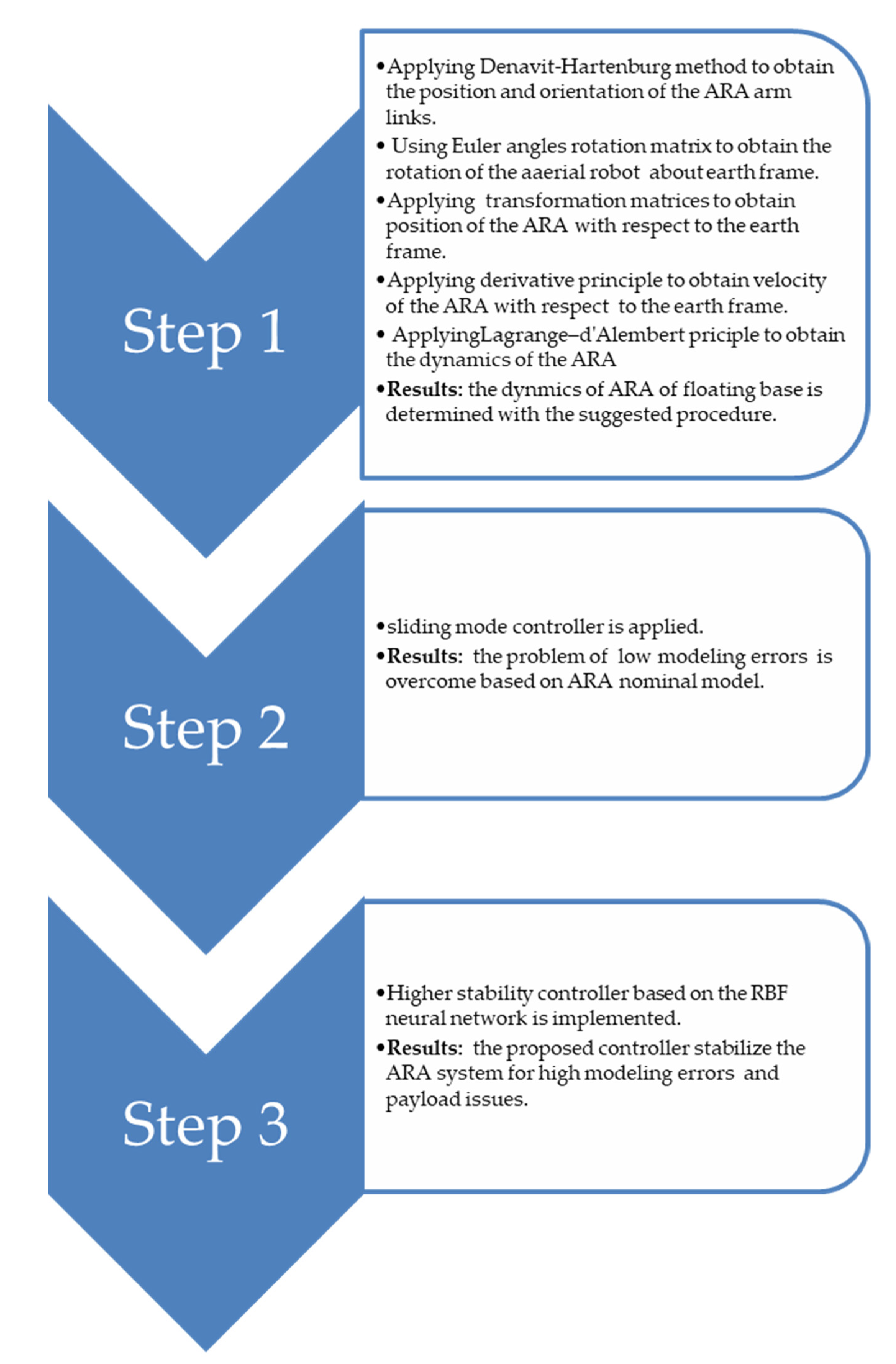
In this paper, a two degree of freedom serial ARA of rotating joints that is mounted on the body of an aerial robot is studied. Unlike the traditional robot manipulators found on fixed or mobile ground robots, the kinematics of the ARA is obtained based on Euler angles and the Denavit–Hartenburg method while considering that the base of the ARA is a float. The dynamics of the ARA are derived in detail using the Lagrange–d’Alembert method. An adaptive robust controller-based Radial Basis Function (RBF) neural network is designed to treat all the mentioned issues in ARA manipulators. The methodology used in this work is summarized in Figure 1.

First, an adaptive robust controller is developed, based on the ARA nominal model and sliding mode control, to overcome the problem of low modeling errors. Second, the RBF neural network of a Gaussian function type is used in the first controller to manage the problem of high modeling errors and disturbances. An additional study is implemented with the second controller that uses RBF neural networks to show the advantage of including RBF neural networks. The validity of the designed controllers is proved using numerical simulations.

The rest of this paper is organized as follows. The related work is discussed in Section 2. Kinematics and dynamics analyses of the ARA are derived in Section 3. Then, in Section 4, a robust controller is developed to manipulate the problem of uncertainties using the nominal mode. Next, in Section 5, the RBF neural network is implemented into adaptive robust controllers to avoid control chattering in situations of high uncertainty (due to modeling error) and disturbances. In Section 6, stability analysis based on a Lyapunov function is discussed. In Section 7, the simulation results are presented. Finally, Section 8 concludes this study by discussing the results and recommendations for future works.

2. Related Work

This section discusses a state of the art, existing work on ARM control. In [18], the momentum of the dynamic model of ARA is considered for an aerial robot by proposing feedback of a torque control type. They developed controllers to show its stability under the assumption of the non-singularity of the aerial robot. A method called “product of exponentials” that considers the ARA position level is implemented in [19] to obtain the kinematics of the ARA and to calculate joint angles of ARA rapidly. In [20], an adaptive controller is developed for the ARA considering the existence of uncertainty in both kinematics and dynamics. They introduce a controller that regulates the attitude and tracks the path, of the end effector continuously. In [21], an adaptive controller with a novel formula is presented with existing uncertainty in the ARA model. Furthermore, the combination of the error of trajectory and interaction force is discussed. In [22], a robust controller using a Lyapunov technique is presented for the ARA with a model of underactuated type. This control algorithm manages the complexity included in the dynamics of the ARA due to uncertainty in the parameters. In addition, the introduced robust control algorithm eliminates the need for measuring the acceleration of the base of ARAs. In [23], a workstation including a robotic arm named “BLOCKS’ WORLD” is developed. The concept of artificial intelligence is implemented to control the robotic arm using voice. In [24], an aerial robot is developed that can undertake unsupervised missions for indoor search and rescue. The neural network is implemented in image processing to provide mission capability of a dynamic type. In [25], a new control algorithm for an aerial robot based on the human brain principle is introduced. The control algorithm applies a neural network, swarm, and hybrid swarm intelligence. The neural network is provided the ability to control the aerial robot autonomously. A summary of the related work is presented in

Table 1. Control model parameter coverage.

Paper Reference Number	Kinematic Calculation	Dynamics Model	Disturbances due to Environmental Conditions	Disturbances due to Payload	Coupling Control Loops	High Modeling Errors
[19]	Yes	No	No	No	No	No
[20]	Yes	Yes	Yes	Yes	No	No
[21]	Yes	Yes	No	No	No	Yes
[22]	Yes	Yes	No	No	No	Yes
This paper	Yes	Yes	Yes	Yes	Yes	Yes

.

Equipping aerial robots with ARAs generates several new challenges related to the ability to control ARAs. This is because the dynamics of an ARA are nonlinear, with multiple inputs/outputs and coupled control loops with the aerial robot itself. Moreover, modeling an ARA in control engineering depends on the principles of physics that are derived from the ARA model simplifications. Therefore, it can be assumed that the developed models of ARA do not sufficiently represent the physical system. Another issue to be considered in the control of ARAs is the disturbances due to payloads and environment. For instance, consider an ARA task of moving an object in the air. The ARA is flying without any payload in the beginning. When it carries an object of unknown physical properties, it leads to the necessity of designing a controller that can address such upload conditions. Furthermore, the changes in environmental conditions—e.g., winds—will act as another kind of disturbance that leads to changes in the ARA dynamics. Developing a controller to ensure high performance while taking into account nonlinearity, coupling, modeling errors, and disturbances is a challenge in the ARA control design process. Consequently, advanced controllers, such as adaptive robust controllers, of non-fixed gains are advantageous since they provide firm performance without depending on ARA models, payload, and environmental changes.

3. Modeling

3.1. Kinematics Analysis

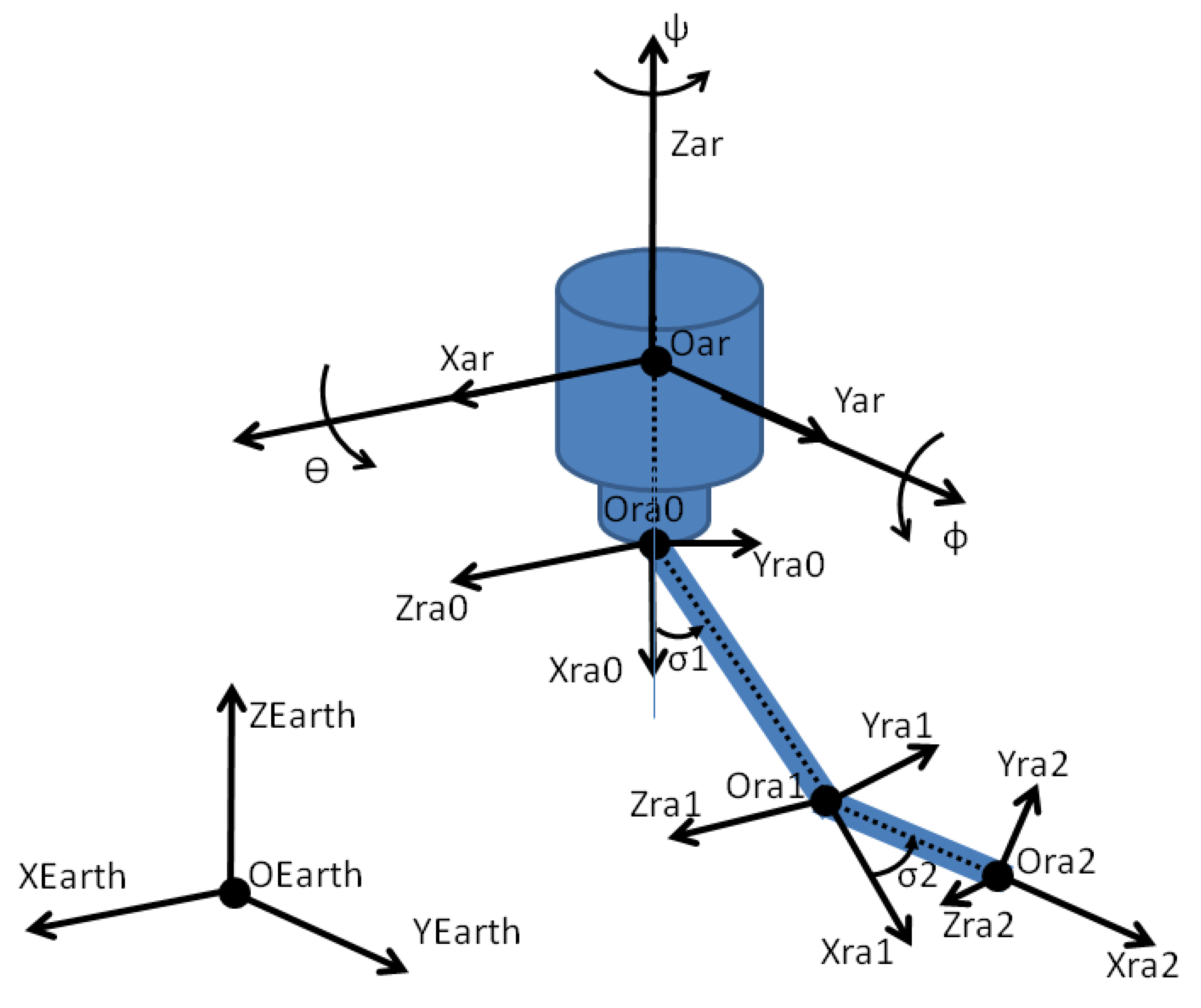
Position and velocity analysis are the two main parts of kinematic modeling. The position of the aerial robot arm links is obtained based on the Denavit–Hartenburg method [26]. Figure 2 presents the kinematics parameters of the system. As can be seen from Figure 2, a two-link aerial robot arm is attached to the body of an aerial robot, assuming the reference frame ${\mathrm{O}}_{\mathrm{ra}}{}_0$ is located on ${\mathrm{O}}_{\mathrm{ra}}$.

Let ${\mathrm{O}}_{\mathrm{Earth}},{ \mathrm{O}}_{\mathrm{ar}},{ \mathrm{O}}_{\mathrm{ra}}{}_{\mathrm{i}}$ be the origin of the reference frames—Earth, aerial robot body, and robot arm links, respectively—where $\mathrm{i}=0,\dots , 2$ represents the joint index of ARA. The joint angles of the aerial robot arm are ${\overline{\mathsf{\Gamma }}}_{\mathrm{ra}}={\left[\begin{array}{cc}{\mathsf{\sigma }}_1& {\mathsf{\sigma }}_2\end{array}\right]}^{\mathrm{T}}$. The body of the aerial robot is orientated by the Euler angles: roll about x-axis $\mathsf{\phi }$, pitch about y-axis $\mathsf{\theta }$, yaw about z-axis$\mathsf{\psi }$; ${\overline{\mathsf{\Gamma }}}_{\mathrm{ar}}=\left[\begin{array}{ccc}\mathsf{\phi }& \mathsf{\theta }& \mathsf{\psi }\end{array}\right]$. By applying the principle of Euler angles [27], the rotation of the aerial robot, with respect to the earth frame, is determined with the following rotation matrix:

$${\mathrm{R}}_{\mathrm{ar}}^{\mathrm{Earth}}=\left[\begin{array}{ccc}\mathrm{c}\mathsf{\psi }\mathrm{c}\mathsf{\theta }& \mathrm{c}\mathsf{\psi }\mathrm{s}\mathsf{\theta }\mathrm{s}\mathsf{\phi }-\mathrm{s}\mathsf{\psi }\mathrm{c}\mathsf{\phi }& \mathrm{c}\mathsf{\psi }\mathrm{s}\mathsf{\theta }\mathrm{c}\mathsf{\phi }+\mathrm{s}\mathsf{\psi }\mathrm{c}\mathsf{\phi }\\ \mathrm{s}\mathsf{\psi }\mathrm{c}\mathsf{\theta }& \mathrm{s}\mathsf{\psi }\mathrm{s}\mathsf{\theta }\mathrm{s}\mathsf{\phi }+\mathrm{c}\mathsf{\psi }\mathrm{c}\mathsf{\phi }& \mathrm{s}\mathsf{\psi }\mathrm{s}\mathsf{\theta }\mathrm{c}\mathsf{\phi }-\mathrm{c}\mathsf{\psi }\mathrm{s}\mathsf{\phi }\\ -\mathrm{s}\mathsf{\theta }& \mathrm{c}\mathsf{\theta }\mathrm{s}\mathsf{\phi }& \mathrm{c}\mathsf{\theta }\mathrm{c}\mathsf{\phi }\end{array}\right],$$

(1)

where the $\mathrm{c}$ and $\mathrm{s}$ denote sine and cosine. The homogeneous transformation matrix that calculates the position and orientation of reference frames ${\mathrm{O}}_{\mathrm{ra}}{}_1$ with respect to ${\mathrm{O}}_{\mathrm{ra}}{}_0$ follows:

$${\mathrm{A}}_1=\left[\begin{array}{cccc}{\mathrm{c}}_1& -{\mathrm{s}}_1& 0& {\mathrm{a}}_1{\mathrm{c}}_1\\ {\mathrm{s}}_1& {\mathrm{c}}_1& 0& {\mathrm{a}}_1{\mathrm{s}}_1\\ 0& 0& 1& 0\\ 0& 0& 0& 1\end{array}\right].$$

(2)

${\mathrm{O}}_{\mathrm{ra}}{}_2$ with respect to ${\mathrm{O}}_{\mathrm{ra}}{}_1$.

$${\mathrm{A}}_2=\left[\begin{array}{cccc}{\mathrm{c}}_2& -{\mathrm{s}}_2& 0& {\mathrm{a}}_2{\mathrm{c}}_2\\ {\mathrm{s}}_2& {\mathrm{c}}_2& 0& {\mathrm{a}}_2{\mathrm{s}}_2\\ 0& 0& 1& 0\\ 0& 0& 0& 1\end{array}\right],$$

(3)

and ${\mathrm{O}}_{\mathrm{ra}}{}_2$ with respect to ${\mathrm{O}}_{\mathrm{ra}}{}_0$.

$${\mathrm{T}}_2^0={\mathrm{A}}_1{\mathrm{A}}_2=\left[\begin{array}{cccc}{\mathrm{c}}_{12}& -{\mathrm{s}}_{12}& 0& {\mathrm{a}}_1{\mathrm{c}}_1+{\mathrm{a}}_2{\mathrm{c}}_{12}\\ {\mathrm{s}}_{12}& {\mathrm{c}}_{12}& 0& {\mathrm{a}}_1{\mathrm{s}}_1+{\mathrm{a}}_2{\mathrm{s}}_{12}\\ 0& 0& 1& 0\\ 0& 0& 0& 1\end{array}\right].$$

(4)

Based on the following assumptions:

• The position of the aerial robot body—i.e., reference frame ${\mathrm{O}}_{\mathrm{ar}}$ position—with respect to the earth frame is:

  $${\mathrm{P}}_{\mathrm{ar}}^{\mathrm{Earth}}={\left[\mathrm{X} \mathrm{Y} \mathrm{Z}\right]}^{\mathrm{T}}.$$

  (5)
• The position of the first link of robot arm end—i.e., reference frame ${\mathrm{O}}_{\mathrm{ra}}{}_1$—relative to the earth frame is:

  $${\mathrm{P}}_{\mathrm{ra}\left(1\right)}^{\mathrm{Earth}}={\mathrm{P}}_{\mathrm{ar}}^{\mathrm{Earth}}+{\mathrm{R}}_{\mathrm{ar}}^{\mathrm{Earth}}{\mathrm{P}}_{\mathrm{ra}\left(1\right)}^{\mathrm{ar}}.$$

  (6)
• The position of the end effector i.e., reference frame ${\mathrm{O}}_{\mathrm{ra}}{}_2$ relative to the earth frame is:

  $${\mathrm{P}}_{\mathrm{ra}\left(2\right)}^{\mathrm{Earth}}={\mathrm{P}}_{\mathrm{ar}}^{\mathrm{Earth}}+{\mathrm{R}}_{\mathrm{ar}}^{\mathrm{Earth}}{\mathrm{P}}_{\mathrm{ra}\left(2\right)}^{\mathrm{ar}}.$$

  (7)

The values of position vectors ${\mathrm{P}}_{\mathrm{ra}\left(1\right)}^{\mathrm{ar}}$ and ${\mathrm{P}}_{\mathrm{ra}\left(2\right)}^{\mathrm{ar}}$ are obtained from the first three rows of the third column of the matrix in Equations (2) and (4), respectively, as below:

$${\mathrm{P}}_{\mathrm{ra}\left(1\right)}^{\mathrm{ar}}={\left[{\mathrm{a}}_1{\mathrm{c}}_1\hspace{1em}{ \mathrm{a}}_1{\mathrm{s}}_1\hspace{1em}0 \right]}^{\mathrm{T}},$$

(8)

$${\mathrm{P}}_{\mathrm{ra}\left(2\right)}^{\mathrm{ar}}={\left[{\mathrm{a}}_1{\mathrm{c}}_1+{\mathrm{a}}_2{\mathrm{c}}_{12}\hspace{1em}{ \mathrm{a}}_1{\mathrm{s}}_1+{\mathrm{a}}_2{\mathrm{s}}_{12}\hspace{1em}0 \right]}^{\mathrm{T}}.$$

(9)

By taking the derivatives of Equations (5)–(7), the linear velocities of the aerial robot body, aerial robot arm (link 1, link 2) will be determined as:

$${\dot{\mathrm{P}}}_{\mathrm{ar}}^{\mathrm{Earth}}={\left[\dot{\mathrm{X}}\dot{\mathrm{Y}}\dot{\mathrm{Z}}\right]}^{\mathrm{T}},$$

(10)

$${\dot{\mathrm{P}}}_{\mathrm{ra}\left(1\right)}^{\mathrm{Earth}}={\dot{\mathrm{P}}}_{\mathrm{ar}}+{\dot{\mathrm{R}}}_{\mathrm{ar}}^{\mathrm{Earth}}{\mathrm{P}}_{\mathrm{ra}\left(1\right)}^{\mathrm{ar}}+{\mathrm{R}}_{\mathrm{ar}}^{\mathrm{Earth}}{\dot{\mathrm{P}}}_{\mathrm{ra}\left(1\right)}^{\mathrm{ar}},$$

(11)

$${\dot{\mathrm{P}}}_{\mathrm{ra}\left(2\right)}^{\mathrm{Earth}}={\dot{\mathrm{P}}}_{\mathrm{ar}}+{\dot{\mathrm{R}}}_{\mathrm{ar}}^{\mathrm{Earth}}{\mathrm{P}}_{\mathrm{ra}\left(2\right)}^{\mathrm{ar}}+{\mathrm{R}}_{\mathrm{ar}}^{\mathrm{Earth}}{\dot{\mathrm{P}}}_{\mathrm{ra}\left(2\right)}^{\mathrm{ar}}.$$

(12)

After considering the linear velocities of the aerial robot arm, with respect to the aerial robot body, in terms of Jacobian matrices and the skew symmetric matrix for rotation matrix, the above equations will be:

$${\dot{\mathrm{P}}}_{\mathrm{ra}\left(1\right)}^{\mathrm{Earth}}={\dot{\mathrm{P}}}_{\mathrm{ar}}+{\mathrm{R}}_{\mathrm{ar}}^{\mathrm{Earth}}\mathrm{SSM}\left({\mathrm{w}}_{\mathrm{ar}}^{\mathrm{Earth}}\right){\mathrm{P}}_{\mathrm{ra}\left(1\right)}^{\mathrm{ar}}+{\mathrm{R}}_{\mathrm{ar}}^{\mathrm{Earth}}{\mathrm{J}}_{\mathrm{v}1}{\dot{\mathsf{\Gamma }}}_{\mathrm{ra}},$$

(13)

$${\dot{\mathrm{P}}}_{\mathrm{ra}\left(2\right)}^{\mathrm{Earth}}={\dot{\mathrm{P}}}_{\mathrm{ar}}+{\mathrm{R}}_{\mathrm{ar}}^{\mathrm{Earth}}\mathrm{SSM}\left({\mathrm{w}}_{\mathrm{ar}}^{\mathrm{Earth}}\right){\mathrm{P}}_{\mathrm{ra}\left(2\right)}^{\mathrm{ar}}+{\mathrm{R}}_{\mathrm{ar}}^{\mathrm{Earth}}{\mathrm{J}}_{\mathrm{v}2}{\dot{\mathsf{\Gamma }}}_{\mathrm{ra}},$$

(14)

On the other hand, the angular velocity of the aerial robot body with respect to the earth frame is:

$${\mathrm{w}}_{\mathrm{ar}}^{\mathrm{Earth}}={\mathrm{R}}_{\mathrm{ar}}^{\mathrm{Earth}}\left[\begin{array}{ccc}1& 0& -\mathrm{s}\mathsf{\theta }\\ 0& \mathrm{c}\mathsf{\phi }& \mathrm{c}\mathsf{\theta }\mathrm{s}\mathsf{\phi }\\ 0& -\mathrm{s}\mathsf{\phi }& \mathrm{c}\mathsf{\theta }\mathrm{c}\mathsf{\phi }\end{array}\right]{\dot{\mathsf{\Gamma }}}_{\mathrm{ar}},$$

(15)

Then, the angular velocities of links with respect to the earth frame are:

$${\mathrm{w}}_{\mathrm{ra}\left(1\right)}^{\mathrm{Earth}}={\mathrm{w}}_{\mathrm{ar}}^{\mathrm{Earth}}+{\mathrm{R}}_{\mathrm{ar}}^{\mathrm{Earth}}{\mathrm{J}}_{\mathrm{w}1}{\dot{\mathsf{\Gamma }}}_{\mathrm{ra}},$$

(16)

$${\mathrm{w}}_{\mathrm{ra}\left(2\right)}^{\mathrm{Earth}}={\mathrm{w}}_{\mathrm{ar}}^{\mathrm{Earth}}+{\mathrm{R}}_{\mathrm{ar}}^{\mathrm{Earth}}{\mathrm{J}}_{\mathrm{w}2}{\dot{\mathsf{\Gamma }}}_{\mathrm{ra}},$$

(17)

where Jacobian matrices of the linear and angular velocities are calculated as:

$${\mathrm{J}}_{\mathrm{v}1}=\left[\begin{array}{cc}-{\mathrm{a}}_1{\mathrm{s}}_1& 0\\ {\mathrm{a}}_1{\mathrm{c}}_1& 0\end{array}\right],$$

$${\mathrm{J}}_{\mathrm{v}2}=\left[\begin{array}{cc}-{\mathrm{a}}_1{\mathrm{s}}_1-{\mathrm{a}}_2{\mathrm{s}}_{12}& -{\mathrm{a}}_2{\mathrm{s}}_{12}\\ {\mathrm{a}}_1{\mathrm{c}}_1+{\mathrm{a}}_2{\mathrm{c}}_{12}& {\mathrm{a}}_2{\mathrm{c}}_{12}\end{array}\right],$$

$${\mathrm{J}}_{\mathrm{w}1}=\left[\begin{array}{cc}1& 0\end{array}\right],$$

$${\mathrm{J}}_{\mathrm{w}2}=\left[\begin{array}{cc}1& 1\end{array}\right].$$

3.2. Dynamics Analysis

The dynamic model of the aerial robot arm is obtained by applying the formula of Lagrange–d’Alembert [28]. This formula is explained as:

$$\frac{\mathrm{d}}{\mathrm{dt}}\left(\frac{\partial \left(\mathrm{K}-\mathrm{U}\right)}{\partial {\dot{\mathsf{\Gamma }}}_{\mathrm{ra}}}\right)-\frac{\partial \left(\mathrm{K}-\mathrm{U}\right)}{\partial {\mathsf{\Gamma }}_{\mathrm{ra}}}={\mathrm{T}}_{\mathrm{in}}-{\overline{\mathrm{T}}}_{\mathrm{ext}},$$

(18)

where K and U represent the kinetic and potential energies of the aerial robot arm, respectively. ${\overline{\mathrm{T}}}_{\mathrm{in}}$ and ${\overline{\mathrm{T}}}_{\mathrm{ext}}$ are the torques of the joints and disturbances, respectively. The vector of joint torques is:

$${\overline{\mathrm{T}}}_{\mathrm{in}}=\left[\begin{array}{cc}{\mathsf{\tau }}_1& {\mathsf{\tau }}_2\end{array}\right].$$

(19)

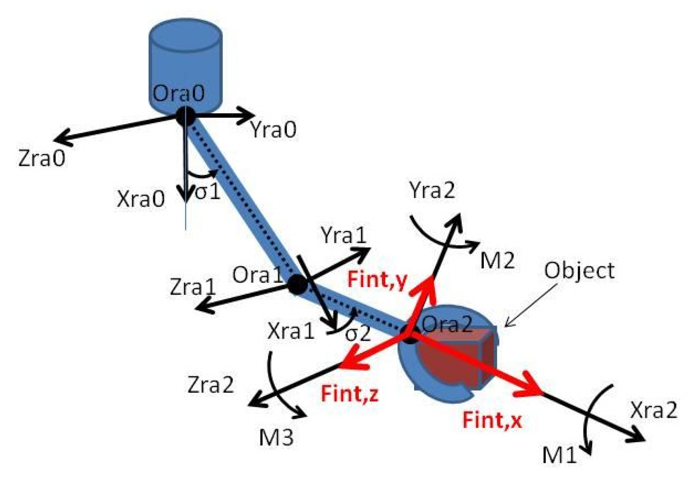
The vector of the disturbances is:

$$T_{ext}=\left[\begin{array}{cccccc}1& 0& 0& 0& 0& 0\\ 0& 1& 0& 0& 0& 0\\ 0& 0& 1& 0& 0& 0\\ 0& 0& a_1{s}_1+a_2{s}_{12}& 1& 0& 0\\ 0& 0& -a_1{c}_1-a_2{c}_{12}& 0& 1& 0\\ a_1{s}_1+a_2{s}_{12}& a_1{c}_1+a_2{c}_{12}& 0& 0& 0& 1\end{array}\right]V.$$

(20)

V is the vector of the interaction force and moments shown in Figure 3 that resulted from holding objects by the end effector.

$$\mathrm{V}={\left[{\mathrm{F}}_{\mathrm{int},\mathrm{x}}{ \mathrm{F}}_{\mathrm{int}, \mathrm{y}}{ \mathrm{F}}_{\mathrm{int}, \mathrm{z}}{ \mathrm{M}}_1{ \mathrm{M}}_2{ \mathrm{M}}_3 \right]}^{\mathrm{T}},$$

where ${\mathrm{F}}_{\mathrm{int}, \mathrm{x}}$, ${\mathrm{F}}_{\mathrm{int}, \mathrm{y}}$, and ${\mathrm{F}}_{\mathrm{int}, \mathrm{z}}$ are the interaction force in the x, y, and z directions, respectively. On the other hand,${ \mathrm{M}}_1$, ${ \mathrm{M}}_2 ,$ and${ \mathrm{M}}_3$ denote the moment resulting from the held object on the x, y, and z axes, respectively.

The total kinetic energy is the summation of the kinetic energy of link 1 (${\mathrm{m}}_{\mathrm{ra}\left(1\right)}$) mass and link 2 (${\mathrm{m}}_{\mathrm{ra}\left(2\right)}$) mass:

$$\mathrm{K}={\mathrm{K}}_{\mathrm{ra}\left(1\right)}+{\mathrm{K}}_{\mathrm{ra}\left(2\right)},$$

(21)

$${\mathrm{K}}_{\mathrm{ra}\left(1\right)}=\frac{1}{2}{\dot{\mathrm{P}}}_{\mathrm{ra}\left(1\right)}^{\mathrm{Earth}}{}^{\mathrm{T}}{\mathrm{m}}_{\mathrm{ra}\left(1\right)}{\dot{\mathrm{P}}}_{\mathrm{ra}\left(1\right)}^{\mathrm{Earth}}+\frac{1}{2}{\mathrm{w}}_1^{\mathrm{Earth}}{}^{\mathrm{T}}{\hat{\mathrm{I}}}_{\mathrm{ar}}{\mathrm{w}}_1^{\mathrm{Earth}},$$

(22)

$${\mathrm{K}}_{\mathrm{ra}\left(2\right)}=\frac{1}{2}{\dot{\mathrm{P}}}_{\mathrm{ra}\left(2\right)}^{\mathrm{Earth}}{}^{\mathrm{T}}{\mathrm{m}}_{\mathrm{ra}\left(2\right)}{\dot{\mathrm{P}}}_{\mathrm{ra}\left(2\right)}^{\mathrm{Earth}}+\frac{1}{2}{\mathrm{w}}_2^{\mathrm{Earth}}{}^{\mathrm{T}}{\hat{\mathrm{I}}}_{\mathrm{ar}}{\mathrm{w}}_2^{\mathrm{Earth}}.$$

(23)

$\hat{\mathrm{I}}$ is the constant inertia matrix at the corresponding reference frames of the aerial robot body and the links of the ARA. The potential energy of the aerial robot arm is the summation of the potential energy of its links:

$$\mathrm{U}={\mathrm{U}}_{\mathrm{ra}\left(1\right)}+{\mathrm{U}}_{\mathrm{ra}\left(2\right)},$$

(24)

$${\mathrm{U}}_{\mathrm{ra}\left(1\right)}={\mathrm{m}}_{\mathrm{ra}\left(1\right)}{\mathrm{gh}}_{\mathrm{ra}\left(1\right)},$$

$${\mathrm{U}}_{\mathrm{ra}\left(2\right)}={\mathrm{m}}_{\mathrm{ra}\left(2\right)}{\mathrm{gh}}_{\mathrm{ra}\left(2\right)},$$

$${\mathrm{h}}_{\mathrm{ra}\left(1\right)}=-{\mathrm{a}}_1\cos \left({\mathsf{\sigma }}_1\right),$$

$${\mathrm{h}}_{\mathrm{ra}\left(2\right)}=-{\mathrm{a}}_1\cos \left({\mathsf{\sigma }}_1\right)-{\mathrm{a}}_2\cos \left({\mathsf{\sigma }}_2\right).$$

By inserting Equations (21) and (24) into Equation (18) yields the following dynamic equation of the ARA:

$${\mathrm{M}}_{\mathrm{ra}}\left({\mathsf{\Gamma }}_{\mathrm{ra}}\right){\ddot{\mathsf{\Gamma }}}_{\mathrm{ra}}+{\mathrm{C}}_{\mathrm{ra}}\left({\mathsf{\Gamma }}_{\mathrm{ra}},{\dot{\mathsf{\Gamma }}}_{\mathrm{ra}}\right){\dot{\mathsf{\Gamma }}}_{\mathrm{ra}}+{\mathrm{G}}_{\mathrm{ra}}\left({\mathsf{\Gamma }}_{\mathrm{ra}}\right)={\mathrm{T}}_{\mathrm{in}}-{\overline{\mathrm{T}}}_{\mathrm{ext}},$$

(25)

where the terms${ \mathrm{M}}_{\mathrm{ra}}\left({\mathsf{\Gamma }}_{\mathrm{ra}}\right)$, ${\mathrm{C}}_{\mathrm{ra}}\left({\mathsf{\Gamma }}_{\mathrm{ra}},{\dot{\mathsf{\Gamma }}}_{\mathrm{ra}}\right)$, ${\mathrm{G}}_{\mathrm{ra}}\left({\mathsf{\Gamma }}_{\mathrm{ra}}\right)$, ${\mathrm{T}}_{\mathrm{in}}$, and ${\overline{\mathrm{T}}}_{\mathrm{ext}}$ denote the centrifugal, Cariolis, gravitational forces, input torques, and disturbances of the ARA joints, respectively.

4. Robust Control Based on Nominal Mode

Considering the dynamic formula of the aerial robot in Equation (25), practically, there are usually modeling errors in obtaining the mathematical expression of${ \mathrm{M}}_{\mathrm{ra}}\left({\mathsf{\Gamma }}_{\mathrm{ra}}\right)$, ${\mathrm{C}}_{\mathrm{ra}}\left({\mathsf{\Gamma }}_{\mathrm{ra}},{\dot{\mathsf{\Gamma }}}_{\mathrm{ra}}\right)$, ${\mathrm{G}}_{\mathrm{ra}}\left({\mathsf{\Gamma }}_{\mathrm{ra}}\right)$. Hence, there are usually unknowns that can be represented as:

$${\mathrm{M}}_{\mathrm{ra}}\left({\mathsf{\Gamma }}_{\mathrm{ra}}\right)=\mathrm{E}\_{\mathrm{M}}_{\mathrm{ra}}+{\mathrm{M}}_{\mathrm{C}}\left({\mathsf{\Gamma }}_{\mathrm{ra}}\right),$$

(26)

$${\mathrm{C}}_{\mathrm{ra}}\left({\mathsf{\Gamma }}_{\mathrm{ra}},{\dot{\mathsf{\Gamma }}}_{\mathrm{ra}}\right)=\mathrm{E}\_{\mathrm{C}}_{\mathrm{ra}}+{\mathrm{C}}_{\mathrm{C}}\left({\mathsf{\Gamma }}_{\mathrm{ra}},{\dot{\mathsf{\Gamma }}}_{\mathrm{ra}}\right),$$

(27)

$${\mathrm{G}}_{\mathrm{ra}}\left({\mathsf{\Gamma }}_{\mathrm{ra}}\right)=\mathrm{E}\_{\mathrm{G}}_{\mathrm{ra}}+{\mathrm{G}}_{\mathrm{C}}\left({\mathsf{\Gamma }}_{\mathrm{ra}}\right),$$

(28)

where ${\mathrm{M}}_{\mathrm{C}}\left({\mathsf{\Gamma }}_{\mathrm{ra}}\right)$, ${\mathrm{C}}_{\mathrm{C}}\left({\mathsf{\Gamma }}_{\mathrm{ra}},{\dot{\mathsf{\Gamma }}}_{\mathrm{ra}}\right)$, and ${\mathrm{G}}_{\mathrm{C}}\left({\mathsf{\Gamma }}_{\mathrm{ra}}\right)$ are the calculated mathematical representations of ${\mathrm{M}}_{\mathrm{ra}}\left({\mathsf{\Gamma }}_{\mathrm{ra}}\right)$, ${\mathrm{C}}_{\mathrm{ra}}\left({\mathsf{\Gamma }}_{\mathrm{ra}},{\dot{\mathsf{\Gamma }}}_{\mathrm{ra}}\right)$, and ${\mathrm{G}}_{\mathrm{ra}}\left({\mathsf{\Gamma }}_{\mathrm{ra}}\right)$, respectively. The$\mathrm{E}\_{\mathrm{M}}_{\mathrm{ra}}$,$\mathrm{E}\_{\mathrm{C}}_{\mathrm{ra}}$, and $\mathrm{E}\_{\mathrm{G}}_{\mathrm{ra}}$ are the modeling errors of ${\mathrm{M}}_{\mathrm{ra}}\left({\mathsf{\Gamma }}_{\mathrm{ra}}\right)$, ${\mathrm{C}}_{\mathrm{ra}}\left({\mathsf{\Gamma }}_{\mathrm{ra}},{\dot{\mathsf{\Gamma }}}_{\mathrm{ra}}\right)$, and ${\mathrm{G}}_{\mathrm{ra}}\left({\mathsf{\Gamma }}_{\mathrm{ra}}\right)$, respectively. Sliding mode control is a vital technique for controlling nonlinear systems that have moderate modeling errors robustly [29]. To design the robust controller, for a desired position ${\mathsf{\Gamma }}_{\mathrm{ra}}{}_{\mathrm{d}}\left(\mathrm{t}\right)$ and actual position value${\mathsf{\Gamma }}_{\mathrm{ra}}\left(\mathrm{t}\right)$, let us first assume the error in tracking as:

$$\mathrm{e}\left(\mathrm{t}\right)={ \mathsf{\Gamma }}_{\mathrm{ra}}{}_{\mathrm{d}}\left(\mathrm{t}\right)-{\mathsf{\Gamma }}_{\mathrm{ra}}\left(\mathrm{t}\right).$$

(29)

Then, for $>0$, the sliding mode formula is designed as:

$$\mathrm{\beth }=\dot{\mathrm{e}}+\mathsf{\mu }\mathrm{e}.$$

(30)

In terms of robustness$\mathrm{\beth }$, the velocity and acceleration of the ARA assumed as ${\dot{\mathsf{\Gamma }}}_{\mathrm{ra}}{}_{\mathrm{\beth }}=\mathrm{\beth }\left(\mathrm{t}\right)+{\dot{\mathsf{\Gamma }}}_{\mathrm{ra}}\left(\mathrm{t}\right)$, ${\ddot{\mathsf{\Gamma }}}_{\mathrm{ra}}{}_{\mathrm{\beth }}=\dot{\mathrm{\beth }}\left(\mathrm{t}\right)+{\ddot{\mathsf{\Gamma }}}_{\mathrm{ra}}\left(\mathrm{t}\right)$, respectively. From these two formulas and Equations (29) and (30), the values of velocity and acceleration of the ARA while considering the slide mode control are: ${\dot{\mathsf{\Gamma }}}_{\mathrm{ra}}{}_{\mathrm{\beth }}={\dot{\mathsf{\Gamma }}}_{\mathrm{ra}}{}_{\mathrm{d}}+\mathsf{\mu }\mathrm{e}$ and ${\ddot{\mathsf{\Gamma }}}_{\mathrm{ra}}{}_{\mathrm{\beth }}={\ddot{\mathsf{\Gamma }}}_{\mathrm{ra}}{}_{\mathrm{d}}+\mathsf{\mu }\dot{\mathrm{e}}$.

Now, referring to Equation (24), the input torque to the ARA is calculated as:

$$\begin{gathered} {\mathrm{T}}_{\mathrm{in}}={\mathrm{M}}_{\mathrm{ra}}\left({\mathsf{\Gamma }}_{\mathrm{ra}}\right){\ddot{\mathsf{\Gamma }}}_{\mathrm{ra}}+{\mathrm{C}}_{\mathrm{ra}}\left({\mathsf{\Gamma }}_{\mathrm{ra}},{\dot{\mathsf{\Gamma }}}_{\mathrm{ra}}\right){\dot{\mathsf{\Gamma }}}_{\mathrm{ra}}+{\mathrm{G}}_{\mathrm{ra}}\left({\mathsf{\Gamma }}_{\mathrm{ra}}\right)+{\overline{\mathrm{T}}}_{\mathrm{ext}}\mathrm{ }={\mathrm{M}}_{\mathrm{ra}}\left({\mathsf{\Gamma }}_{\mathrm{ra}}\right)\left({\ddot{\mathsf{\Gamma }}}_{\mathrm{ra}}{}_{\mathrm{r}}-\dot{\mathrm{\beth }}\right)+ \\ {\mathrm{C}}_{\mathrm{ra}}\left({\mathsf{\Gamma }}_{\mathrm{ra}},{\dot{\mathsf{\Gamma }}}_{\mathrm{ra}}\right)\left({\dot{\mathsf{\Gamma }}}_{\mathrm{ra}}{}_{\mathrm{r}}-\mathrm{\beth }\right)+{\mathrm{G}}_{\mathrm{ra}}\left({\mathsf{\Gamma }}_{\mathrm{ra}}\right)+{\overline{\mathrm{T}}}_{\mathrm{ext}}={\mathrm{M}}_{\mathrm{ra}}\left({\mathsf{\Gamma }}_{\mathrm{ra}}\right){\ddot{\mathsf{\Gamma }}}_{\mathrm{ra}}{}_{\mathrm{r}}+{\mathrm{C}}_{\mathrm{ra}}\left({\mathsf{\Gamma }}_{\mathrm{ra}},{\dot{\mathsf{\Gamma }}}_{\mathrm{ra}}\right){\dot{\mathsf{\Gamma }}}_{\mathrm{ra}}{}_{\mathrm{r}}+ \\ {\mathrm{G}}_{\mathrm{ra}}\left({\mathsf{\Gamma }}_{\mathrm{ra}}\right)-{\mathrm{M}}_{\mathrm{ra}}\left({\mathsf{\Gamma }}_{\mathrm{ra}}\right)\dot{\mathrm{\beth }}-{\mathrm{C}}_{\mathrm{ra}}\left({\mathsf{\Gamma }}_{\mathrm{ra}},{\dot{\mathsf{\Gamma }}}_{\mathrm{ra}}\right)\mathrm{\beth }+{\overline{\mathrm{T}}}_{\mathrm{ext}}\mathrm{ }={\mathrm{M}}_{\mathrm{C}}\left({\mathsf{\Gamma }}_{\mathrm{ra}}\right){\ddot{\mathsf{\Gamma }}}_{\mathrm{ra}}{}_{\mathrm{r}}+{\mathrm{C}}_{\mathrm{C}}\left({\mathsf{\Gamma }}_{\mathrm{ra}},{\dot{\mathsf{\Gamma }}}_{\mathrm{ra}}\right){\dot{\mathsf{\Gamma }}}_{\mathrm{ra}}{}_{\mathrm{r}}+ \\ {\mathrm{G}}_{\mathrm{C}}\left({\mathsf{\Gamma }}_{\mathrm{ra}}\right)+{\mathrm{E}}_{{\mathrm{M}}_{\mathrm{ra}}}{\ddot{\mathsf{\Gamma }}}_{\mathrm{ra}}{}_{\mathrm{r}}+{\mathrm{E}}_{{\mathrm{C}}_{\mathrm{ra}}}{\dot{\mathsf{\Gamma }}}_{\mathrm{ra}}{}_{\mathrm{r}}+\mathrm{E}\_{\mathrm{G}}_{\mathrm{ra}}-{\mathrm{M}}_{\mathrm{ra}}\left({\mathsf{\Gamma }}_{\mathrm{ra}}\right)\dot{\mathrm{\beth }}-{\mathrm{C}}_{\mathrm{ra}}\left({\mathsf{\Gamma }}_{\mathrm{ra}},{\dot{\mathsf{\Gamma }}}_{\mathrm{ra}}\right)\mathrm{\beth }+{\overline{\mathrm{T}}}_{\mathrm{ext}} \end{gathered}$$

(31)

In terms of the nominal torque part ${\mathrm{T}}_{\mathrm{N}}$, robust torque part ${\mathrm{T}}_{\mathrm{\beth }}$, proportional gain ${\mathrm{K}}_{\mathrm{p}}>0$, and integral gain ${\mathrm{K}}_{\mathrm{i}}>0$, the input torque to the ARA is:

$${\mathrm{T}}_{\mathrm{in}}={\mathrm{T}}_{\mathrm{N}}+{\mathrm{T}}_{\mathrm{\beth }}+{\mathrm{K}}_{\mathrm{p}}\mathrm{\beth }+{\mathrm{K}}_{\mathrm{i}}{{\displaystyle \int }}^{ }\mathrm{\beth }\mathrm{dt},$$

(32)

where:

$${\mathrm{M}}_{\mathrm{C}}\left({\mathsf{\Gamma }}_{\mathrm{ra}}\right){\ddot{\mathsf{\Gamma }}}_{\mathrm{ra}}{}_{\mathrm{\beth }}+{\mathrm{C}}_{\mathrm{C}}\left({\mathsf{\Gamma }}_{\mathrm{ra}},{\dot{\mathsf{\Gamma }}}_{\mathrm{ra}}\right){\dot{\mathsf{\Gamma }}}_{\mathrm{ra}}{}_{\mathrm{\beth }}+{\mathrm{G}}_{\mathrm{C}}\left({\mathsf{\Gamma }}_{\mathrm{ra}}\right),$$

(33)

Then:

$${\mathrm{T}}_{\mathrm{\beth }}={\mathrm{K}}_{\mathrm{\beth }}\mathrm{sgn}\left(\mathrm{\beth }\right).$$

(34)

Inserting Equations (33) and (34) into Equation (32) and substituting the latter into Equation (31) results in the following dynamics equation of the ARA:

$$\begin{gathered} {\mathrm{M}}_{\mathrm{ra}}\left({\mathsf{\Gamma }}_{\mathrm{ra}}\right)\dot{\mathrm{\beth }}+{\mathrm{C}}_{\mathrm{ra}}\left({\mathsf{\Gamma }}_{\mathrm{ra}},{\dot{\mathsf{\Gamma }}}_{\mathrm{ra}}\right)\mathrm{\beth }+{\mathrm{K}}_{\mathrm{i}}\int \mathrm{\beth }\mathrm{dt}=-{\mathrm{K}}_{\mathrm{p}}\mathrm{\beth }-{\mathrm{K}}_{\mathrm{\beth }}\mathrm{sgn}\left(\mathrm{\beth }\right)+{\mathrm{E}}_{{\mathrm{M}}_{\mathrm{ra}}}{\ddot{\mathsf{\Gamma }}}_{\mathrm{ra}}{}_{\mathrm{r}} \\ +{\mathrm{E}}_{{\mathrm{C}}_{\mathrm{ra}}}{\dot{\mathsf{\Gamma }}}_{\mathrm{ra}}{}_{\mathrm{r}}+{\mathrm{E}}_{{\mathrm{G}}_{\mathrm{ra}}}+{\mathrm{K}}_{\mathrm{\beth }}\mathrm{sgn}\left(\mathrm{\beth }\right). \end{gathered}$$

(35)

The drawback of the robust controller is that the nominal model of the ARA should be calculated. Besides this, the big errors in the model yield a large ${\mathrm{K}}_{\mathrm{\beth }\mathrm{jj}}$. In turn, high control chattering is produced [30,31]. To avoid this issue, an RBF neural network will be applied.

5. Adaptive RBF Neural Network Control

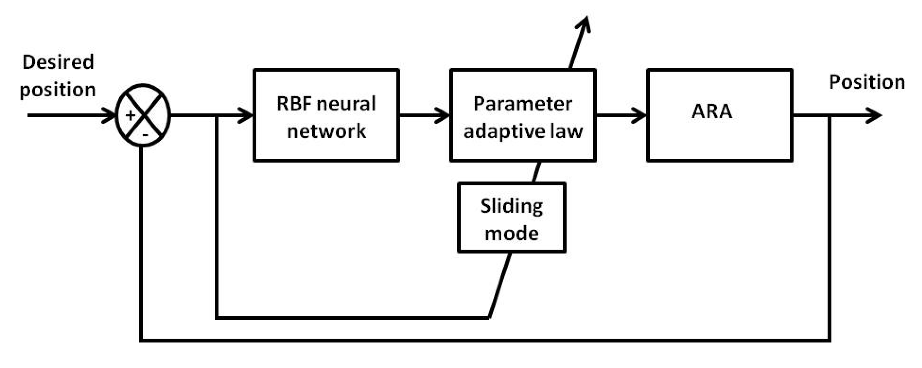
An inexact ARA model causes tracking errors [32]. To enhance the tracking performance of our designed robust controller in the presence of high modeling errors and disturbances of the ARA, an RBF neural network, as an artificial intelligence approach, is implemented due to its learning and mapping abilities [33,34]. The RBF neural network, as shown in Figure 4, is applied to compensate for the errors in ${\mathrm{M}}_{\mathrm{NN}}\left({\mathsf{\Gamma }}_{\mathrm{ra}}\right)$, ${\mathrm{C}}_{\mathrm{NN}}\left({\mathsf{\Gamma }}_{\mathrm{ra}},{\dot{\mathsf{\Gamma }}}_{\mathrm{ra}}\right)$, and ${\mathrm{G}}_{\mathrm{NN}}\left({\mathsf{\Gamma }}_{\mathrm{ra}}\right)$.

In turn, the modeling errors will be approximated and the accuracy of the tracking control will be improved. The structure of the RBF neural network has two inputs, three hidden layers, and one output. The RBF NN of output ${\mathrm{M}}_{\mathrm{NN}}\left({\mathsf{\Gamma }}_{\mathrm{ra}}\right)$, ${\mathrm{C}}_{\mathrm{NN}}\left({\mathsf{\Gamma }}_{\mathrm{ra}},{\dot{\mathsf{\Gamma }}}_{\mathrm{ra}}\right)$, and ${\mathrm{G}}_{\mathrm{NN}}\left({\mathsf{\Gamma }}_{\mathrm{ra}}\right)$ is applied to model${ \mathrm{M}}_{\mathrm{ra}}\left({\mathsf{\Gamma }}_{\mathrm{ra}}\right)$, ${\mathrm{C}}_{\mathrm{ra}}\left({\mathsf{\Gamma }}_{\mathrm{ra}},{\dot{\mathsf{\Gamma }}}_{\mathrm{ra}}\right)$, and ${\mathrm{G}}_{\mathrm{ra}}\left({\mathsf{\Gamma }}_{\mathrm{ra}}\right).$ Regarding the NN weight and hidden layers, the ideal weight value of RBF is assumed ${\mathrm{W}}_{{\mathrm{M}}_{\mathrm{ra}}}$, ${\mathrm{W}}_{{\mathrm{C}}_{\mathrm{ra}}}$, and ${\mathrm{W}}_{{\mathrm{G}}_{\mathrm{ra}}},$ while the output of the hidden layers is ${\mathrm{H}}_{{\mathrm{M}}_{\mathrm{ra}}}$, ${\mathrm{H}}_{{\mathrm{C}}_{\mathrm{ra}}}$, and ${\mathrm{H}}_{{\mathrm{G}}_{\mathrm{ra}}}$.

Thus,

$${\mathrm{M}}_{\mathrm{ra}}\left({\mathsf{\Gamma }}_{\mathrm{ra}}\right)=\mathrm{E}\_{\mathrm{M}}_{\mathrm{ra}}+{\mathrm{M}}_{\mathrm{NN}}\left({\mathsf{\Gamma }}_{\mathrm{ra}}\right),$$

(36)

$${\text{C}}_{\text{ra}}\left({\text{Γ}}_{\text{ra}}\right)=\text{E}\_{\text{C}}_{\text{ra}}+{\text{C}}_{\text{NN}}\left({\text{Γ}}_{\text{ra}}\right),$$

(37)

$${\text{G}}_{\text{ra}}\left({\text{Γ}}_{\text{ra}}\right)=\text{E}\_{\text{G}}_{\text{ra}}+{\text{G}}_{\text{NN}}\left({\text{Γ}}_{\text{ra}}\right),$$

(38)

Inserting the above equations in the dynamics formula of the ARA—i.e., Equation (25)—results in:

$$\begin{gathered} {\mathrm{M}}_{\mathrm{ra}}\left({\mathsf{\Gamma }}_{\mathrm{ra}}\right){\ddot{\mathsf{\Gamma }}}_{\mathrm{ra}}{}_{\mathrm{\beth }}+{\mathrm{C}}_{\mathrm{ra}}\left({\mathsf{\Gamma }}_{\mathrm{ra}},{\dot{\mathsf{\Gamma }}}_{\mathrm{ra}}\right){\dot{\mathsf{\Gamma }}}_{\mathrm{ra}}{}_{\mathrm{\beth }}+{\mathrm{G}}_{\mathrm{ra}}\left({\mathsf{\Gamma }}_{\mathrm{ra}}\right)={\mathrm{E}}_{{\mathrm{M}}_{\mathrm{ra}}}{\ddot{\mathsf{\Gamma }}}_{\mathrm{ra}}{}_{\mathrm{\beth }}+{\mathrm{E}}_{{\mathrm{C}}_{\mathrm{ra}}}{\dot{\mathsf{\Gamma }}}_{\mathrm{ra}}{}_{\mathrm{\beth }}+{\mathrm{E}}_{{\mathrm{G}}_{\mathrm{ra}}}+{\mathrm{T}}_{\mathrm{ext}}+ \\ {\mathrm{M}}_{\mathrm{NN}}\left({\mathsf{\Gamma }}_{\mathrm{ra}}\right){\ddot{\mathsf{\Gamma }}}_{\mathrm{ra}}{}_{\mathrm{\beth }}+{\mathrm{C}}_{\mathrm{NN}}\left({\mathsf{\Gamma }}_{\mathrm{ra}},{\dot{\mathsf{\Gamma }}}_{\mathrm{ra}}\right){\dot{\mathsf{\Gamma }}}_{\mathrm{ra}}{}_{\mathrm{\beth }}+{\mathrm{C}}_{\mathrm{NN}}\left({\mathsf{\Gamma }}_{\mathrm{ra}},{\dot{\mathsf{\Gamma }}}_{\mathrm{ra}}\right)={\mathrm{E}}_{{\mathrm{M}}_{\mathrm{ra}}}{\ddot{\mathsf{\Gamma }}}_{\mathrm{ra}}{}_{\mathrm{\beth }}+{\mathrm{E}}_{{\mathrm{C}}_{\mathrm{ra}}}{\dot{\mathsf{\Gamma }}}_{\mathrm{ra}}{}_{\mathrm{\beth }}+{\mathrm{E}}_{{\mathrm{G}}_{\mathrm{ra}}}+ \\ \left[{\left\{{\mathrm{W}}_{{\mathrm{M}}_{\mathrm{ra}}}\right\}}^{\mathrm{T}}.\left\{{\mathrm{H}}_{{\mathrm{M}}_{\mathrm{ra}}}\left({\mathsf{\Gamma }}_{\mathrm{ra}}\right)\right\}\right]{\ddot{\mathsf{\Gamma }}}_{\mathrm{ra}}{}_{\mathrm{\beth }}+\left[{\left\{{\mathrm{W}}_{{\mathrm{C}}_{\mathrm{ra}}}\right\}}^{\mathrm{T}}.\left\{{\mathrm{H}}_{{\mathrm{C}}_{\mathrm{ra}}}\left({\mathsf{\Gamma }}_{\mathrm{ra}},{\dot{\mathsf{\Gamma }}}_{\mathrm{ra}}\right)\right\}\right]{\dot{\mathsf{\Gamma }}}_{\mathrm{ra}}{}_{\mathrm{\beth }}+\left[\left[{\left\{{\mathrm{W}}_{{\mathrm{G}}_{\mathrm{ra}}}\right\}}^{\mathrm{T}}.\left\{{\mathrm{H}}_{{\mathrm{G}}_{\mathrm{ra}}}\left({\mathsf{\Gamma }}_{\mathrm{ra}}\right)\right\}\right]\right] \end{gathered}$$

(39)

Then, the estimation of${ \mathrm{M}}_{\mathrm{NN}}\left({\mathsf{\Gamma }}_{\mathrm{ra}}\right)$, ${\mathrm{C}}_{\mathrm{NN}}$, and ${\mathrm{G}}_{\mathrm{NN}}$ will be included to confirm data and model forecasting for modeling errors. In terms of RBF, the estimation of mismatch between the calculated and nominal values is supposed as:

$${\hat{\mathrm{M}}}_{\mathrm{NN}}\left({\mathsf{\Gamma }}_{\mathrm{ra}}\right)=\left[{\left\{{\hat{\mathrm{W}}}_{{\mathrm{M}}_{\mathrm{ra}}}\right\}}^{\mathrm{T}}.\left\{{\mathrm{E}}_{{\mathrm{M}}_{\mathrm{ra}}}\left({\mathsf{\Gamma }}_{\mathrm{ra}}\right)\right\}\right],$$

(40)

$${\hat{\mathrm{C}}}_{\mathrm{NN}}\left({\mathsf{\Gamma }}_{\mathrm{ra}}\right)=\left[{\left\{{\hat{\mathrm{W}}}_{{\mathrm{C}}_{\mathrm{ra}}}\right\}}^{\mathrm{T}}.\left\{{\mathrm{E}}_{{\mathrm{C}}_{\mathrm{ra}}}\left({\mathsf{\Gamma }}_{\mathrm{ra}},{\dot{\mathsf{\Gamma }}}_{\mathrm{ra}}\right)\right\}\right],$$

(41)

$${\hat{\mathrm{G}}}_{\mathrm{NN}}\left({\mathsf{\Gamma }}_{\mathrm{ra}}\right)=\left[{\left\{{\hat{\mathrm{W}}}_{{\mathrm{G}}_{\mathrm{ra}}}\right\}}^{\mathrm{T}}.\left\{{\mathrm{E}}_{{\mathrm{G}}_{\mathrm{ra}}}\left({\mathsf{\Gamma }}_{\mathrm{ra}}\right)\right\}\right],$$

(42)

where ${\hat{\mathrm{W}}}_{{\mathrm{M}}_{\mathrm{ra}}}$,${\hat{\mathrm{W}}}_{{\mathrm{C}}_{\mathrm{ra}}}$, and ${\hat{\mathrm{W}}}_{{\mathrm{G}}_{\mathrm{ra}}}$ are estimates of ${\mathrm{W}}_{{\mathrm{M}}_{\mathrm{ra}}}$, ${\mathrm{W}}_{{\mathrm{C}}_{\mathrm{ra}}}$, and ${\mathrm{W}}_{{\mathrm{G}}_{\mathrm{ra}}}$, respectively. Consequently, the control algorithm of the estimated model is:

$${\mathrm{T}}_{\mathrm{m}}={\hat{\mathrm{M}}}_{\mathrm{NN}}\left({\mathsf{\Gamma }}_{\mathrm{ra}}\right){\ddot{\mathsf{\Gamma }}}_{\mathrm{ra}}{}_{\mathrm{\beth }}+{\hat{\mathrm{C}}}_{\mathrm{NN}}\left({\mathsf{\Gamma }}_{\mathrm{ra}},{\dot{\mathsf{\Gamma }}}_{\mathrm{ra}}\right){\dot{\mathsf{\Gamma }}}_{\mathrm{ra}}{}_{\mathrm{\beth }}+{\mathrm{G}}_{\mathrm{NN}}\left({\mathsf{\Gamma }}_{\mathrm{ra}}\right).$$

(43)

By following the same procedure for the design of a robust controller in Section 4, we obtain:

$$\begin{gathered} {\mathrm{M}}_{\mathrm{ra}}\left({\mathsf{\Gamma }}_{\mathrm{ra}}\right)\dot{\mathrm{\beth }}+{\mathrm{C}}_{\mathrm{ra}}\left({\mathsf{\Gamma }}_{\mathrm{ra}},{\dot{\mathsf{\Gamma }}}_{\mathrm{ra}}\right)\mathrm{\beth }+{\mathrm{K}}_{\mathrm{i}}{{\displaystyle \int }}^{\mathrm{ }}\mathrm{\beth }\mathrm{dt}=-{\mathrm{K}}_{\mathrm{p}}\mathrm{\beth }-{\mathrm{K}}_{\mathrm{\beth }}\mathrm{sgn}\left(\mathrm{\beth }\right)+ \\ \left[{\left\{{\tilde{\mathrm{W}}}_{{\mathrm{M}}_{\mathrm{ra}}}\right\}}^{\mathrm{T}}.\left\{{\mathrm{H}}_{{\mathrm{M}}_{\mathrm{ra}}}\left({\mathsf{\Gamma }}_{\mathrm{ra}}\right)\right\}\right]{\ddot{\mathsf{\Gamma }}}_{\mathrm{ra}}{}_{\mathrm{\beth }}+\left[{\left\{{\tilde{\mathrm{W}}}_{{\mathrm{C}}_{\mathrm{ra}}}\right\}}^{\mathrm{T}}.\left\{{\mathrm{H}}_{{\mathrm{C}}_{\mathrm{ra}}}\left({\mathsf{\Gamma }}_{\mathrm{ra}},{\dot{\mathsf{\Gamma }}}_{\mathrm{ra}}\right)\right\}\right]{\dot{\mathsf{\Gamma }}}_{\mathrm{ra}}{}_{\mathrm{\beth }}+ \\ \left[\left[{\left\{{\tilde{\mathrm{W}}}_{{\mathrm{G}}_{\mathrm{ra}}}\right\}}^{\mathrm{T}}.\left\{{\mathrm{H}}_{{\mathrm{G}}_{\mathrm{ra}}}\left({\mathsf{\Gamma }}_{\mathrm{ra}}\right)\right\}\right]\right]+{\mathrm{E}}_{{\mathrm{M}}_{\mathrm{ra}}}{\ddot{\mathsf{\Gamma }}}_{\mathrm{ra}}{}_{\mathrm{\beth }}+{\mathrm{E}}_{{\mathrm{C}}_{\mathrm{ra}}}{\dot{\mathsf{\Gamma }}}_{\mathrm{ra}}{}_{\mathrm{\beth }}+{\mathrm{E}}_{{\mathrm{G}}_{\mathrm{ra}}} \end{gathered}$$

(44)

where:

$$\begin{gathered} {\tilde{\mathrm{W}}}_{{\mathrm{M}}_{\mathrm{ra}}}={\mathrm{W}}_{{\mathrm{M}}_{\mathrm{ra}}}-{\hat{\mathrm{W}}}_{{\mathrm{M}}_{\mathrm{ra}}}, \\ {\tilde{\mathrm{W}}}_{{\mathrm{C}}_{\mathrm{ra}}}={\mathrm{W}}_{{\mathrm{C}}_{\mathrm{ra}}}-{\hat{\mathrm{W}}}_{{\mathrm{C}}_{\mathrm{ra}}}, \\ {\tilde{\mathrm{W}}}_{{\mathrm{G}}_{\mathrm{ra}}}={\mathrm{W}}_{{\mathrm{G}}_{\mathrm{ra}}}-{\hat{\mathrm{W}}}_{{\mathrm{G}}_{\mathrm{ra}}}. \end{gathered}$$

As the last part of our designed controller, the adaptive rule is set as:

$${\dot{\hat{\mathrm{W}}}}_{{\mathrm{M}}_{\mathrm{rai}}}={\mathrm{ᶘ}}_{{\mathrm{M}}_{\mathrm{rai}}}.\left\{{\mathsf{\zeta }}_{{\mathrm{M}}_{\mathrm{rai}}}\left({\mathsf{\Gamma }}_{\mathrm{ra}}\right)\right\}{\ddot{\mathsf{\Gamma }}}_{\mathrm{ra}}{}_{\mathrm{\beth }}{\mathrm{\beth }}_{\mathrm{I}},$$

(45)

$${\dot{\hat{\mathrm{W}}}}_{{\mathrm{M}}_{\mathrm{rai}}}={\mathrm{ᶘ}}_{{\mathrm{C}}_{\mathrm{rai}}}.\left\{{\mathsf{\zeta }}_{{\mathrm{M}}_{\mathrm{rai}}}\left({\mathsf{\Gamma }}_{\mathrm{ra}}\right)\right\}{\dot{\mathsf{\Gamma }}}_{\mathrm{ra}}{}_{\mathrm{\beth }}{\mathrm{\beth }}_{\mathrm{i}},$$

(46)

$${\dot{\hat{\mathrm{W}}}}_{{\mathrm{M}}_{\mathrm{rai}}}={\mathrm{ᶘ}}_{{\mathrm{C}}_{\mathrm{rai}}}.\left\{{\mathsf{\zeta }}_{{\mathrm{M}}_{\mathrm{rai}}}\left({\mathsf{\Gamma }}_{\mathrm{ra}}\right)\right\}{\mathrm{\beth }}_{\mathrm{i}},$$

(47)

where i = 1, 2; ${\mathrm{ᶘ}}_{{\mathrm{M}}_{\mathrm{rai}}}$, ${\mathrm{ᶘ}}_{{\mathrm{C}}_{\mathrm{rai}}}$, ${\mathrm{ᶘ}}_{{\mathrm{G}}_{\mathrm{rai}}}$ are symmetric matrices of positive and constant elements. To check the ability of our designed controller, explained in this section of operation for large modeling errors, a stability analysis is presented.

6. Stability Analysis

Checking the stability of the ARA manipulator is implemented in the following. Let us assume the integration-type Lyapunov formula [35], which is applied to establish the stability of the ARA:

$$\begin{gathered} \mathrm{V}=\frac{1}{2}{\mathrm{\beth }}^{\mathrm{T}}{\mathrm{M}}_{\mathrm{ra}}\mathrm{\beth }+\frac{1}{2}\left({{\displaystyle \int }}_0^{\mathrm{t}}\mathrm{\beth }{\mathrm{dT}}_{\mathrm{in}}\right){\mathrm{K}}_{\mathrm{I}}\left({{\displaystyle \int }}_0^{\mathrm{t}}\mathrm{\beth }{\mathrm{dT}}_{\mathrm{in}}\right)+\frac{1}{2}{{\displaystyle \sum }}_{\mathrm{k}=1}^2{\tilde{\mathrm{W}}}_{{\mathrm{M}}_{\mathrm{rai}}}^{\mathrm{T}}{\mathrm{ᶘ}}_{{\mathrm{M}}_{\mathrm{rai}}}^{-1}{\tilde{\mathrm{W}}}_{{\mathrm{M}}_{\mathrm{rai}}} \\ +\frac{1}{2}{{\displaystyle \sum }}_{\mathrm{k}=1}^2{\tilde{\mathrm{W}}}_{{\mathrm{C}}_{\mathrm{rai}}}^{\mathrm{T}}{\mathrm{ᶘ}}_{{\mathrm{C}}_{\mathrm{rai}}}^{-1}{\tilde{\mathrm{W}}}_{{\mathrm{C}}_{\mathrm{rai}}}+\frac{1}{2}{{\displaystyle \sum }}_{\mathrm{k}=1}^2{\tilde{\mathrm{W}}}_{{\mathrm{G}}_{\mathrm{rai}}}^{\mathrm{T}}{\mathrm{ᶘ}}_{{\mathrm{G}}_{\mathrm{rai}}}^{-1}{\tilde{\mathrm{W}}}_{{\mathrm{G}}_{\mathrm{rai}}}, \end{gathered}$$

(48)

and its derivative:

$$\begin{gathered} \dot{\mathrm{V}}={\mathrm{\beth }}^{\mathrm{T}}\left[{\mathrm{M}}_{\mathrm{ra}}\dot{\mathrm{\beth }}+\frac{1}{2}{\mathrm{M}}_{\mathrm{ra}}\mathrm{\beth }+{\mathrm{K}}_{\mathrm{I}}\left({{\displaystyle \int }}_0^{\mathrm{t}}\mathrm{\beth }{\mathrm{dT}}_{\mathrm{in}}\right)\right]+{{\displaystyle \sum }}_{\mathrm{k}=1}^2{\tilde{\mathrm{W}}}_{{\mathrm{M}}_{\mathrm{rai}}}^{\mathrm{T}}{\mathrm{ᶘ}}_{{\mathrm{M}}_{\mathrm{rai}}}^{-1}{\dot{\tilde{\mathrm{W}}}}_{{\mathrm{M}}_{\mathrm{rai}}}+ \\ {{\displaystyle \sum }}_{\mathrm{k}=1}^2{\tilde{\mathrm{W}}}_{{\mathrm{C}}_{\mathrm{rai}}}^{\mathrm{T}}{\mathrm{ᶘ}}_{{\mathrm{C}}_{\mathrm{rai}}}^{-1}{\dot{\tilde{\mathrm{W}}}}_{{\mathrm{C}}_{\mathrm{rai}}}+{\displaystyle \sum }_{\mathrm{k}=1}^2{\tilde{\mathrm{W}}}_{{\mathrm{G}}_{\mathrm{rai}}}^{\mathrm{T}}{\mathrm{ᶘ}}_{{\mathrm{G}}_{\mathrm{rai}}}^{-1}{\dot{\tilde{\mathrm{W}}}}_{{\mathrm{G}}_{\mathrm{rai}}}. \end{gathered}$$

(49)

The dynamics of the two-rotating-joints ARA has the property of skew-symmetric—i.e., ${\mathrm{\beth }}^{\mathrm{T}}\left({ \mathrm{M} \dot{}}_{\mathrm{ra}}-2{\mathrm{C}}_{\mathrm{ra}}\mathrm{\beth }\right)=0$.

Thus:

$$\dot{\mathrm{V}}={\mathrm{\beth }}^{\mathrm{T}}\left[{\mathrm{M}}_{\mathrm{ra}}\dot{\mathrm{\beth }}+{\mathrm{C}}_{\mathrm{ra}}\mathrm{\beth }+{\mathrm{K}}_{\mathrm{I}}\left({{\displaystyle \int }}_0^{\mathrm{t}}\mathrm{\beth }{\mathrm{dT}}_{\mathrm{in}}\right)\right].$$

(50)

We inserting the dynamics equation of the ARA into the above equation:

$$\begin{gathered} {\mathrm{\beth }}^{\mathrm{T}}\left[{\left\{{\tilde{\mathrm{W}}}_{{\mathrm{M}}_{\mathrm{ra}}}\right\}}^{\mathrm{T}}.\left\{{\mathrm{H}}_{{\mathrm{M}}_{\mathrm{ra}}}\left({\mathsf{\Gamma }}_{\mathrm{ra}}\right)\right\}\right]{\ddot{\mathsf{\Gamma }}}_{\mathrm{ra}}{}_{\mathrm{\beth }}=\left[\begin{array}{cc}{\mathrm{\beth }}_1& {\mathrm{\beth }}_2\end{array}\right]\left[\begin{array}{c}{\left\{{\tilde{\mathrm{W}}}_{{\mathrm{M}}_{\mathrm{ra}1}}\right\}}^{\mathrm{T}}.\left\{{\mathsf{\zeta }}_{{\mathrm{M}}_{\mathrm{ra}1}}\right\}{\ddot{\mathsf{\Gamma }}}_{\mathrm{ra}}{}_{\mathrm{\beth }}\\ {\left\{{\tilde{\mathrm{W}}}_{{\mathrm{M}}_{\mathrm{ra}2}}\right\}}^{\mathrm{T}}.\left\{{\mathsf{\zeta }}_{{\mathrm{M}}_{\mathrm{ra}2}}\right\}{\ddot{\mathsf{\Gamma }}}_{\mathrm{ra}}{}_{\mathrm{\beth }}\end{array}\right]={\displaystyle \sum }_{\mathrm{j}=1}^2{\left\{{\tilde{\mathrm{W}}}_{{\mathrm{M}}_{\mathrm{raj}}}\right\}}^{\mathrm{T}}.\left\{{\mathsf{\zeta }}_{{\mathrm{M}}_{\mathrm{raj}}}\right\}{\ddot{\mathsf{\Gamma }}}_{\mathrm{ra}}{}_{\mathrm{\beth }}{\mathrm{\beth }}_{\mathrm{j}} \\ {\mathrm{\beth }}^{\mathrm{T}}\left[{\left\{{\tilde{\mathrm{W}}}_{{\mathrm{C}}_{\mathrm{ra}}}\right\}}^{\mathrm{T}}.\left\{{\mathrm{H}}_{{\mathrm{C}}_{\mathrm{ra}}}\left({\mathsf{\Gamma }}_{\mathrm{ra}}\right)\right\}\right]{\dot{\mathsf{\Gamma }}}_{\mathrm{ra}}{}_{\mathrm{\beth }}={\displaystyle \sum }_{\mathrm{j}=1}^2{\left\{{\tilde{\mathrm{W}}}_{{\mathrm{C}}_{\mathrm{raj}}}\right\}}^{\mathrm{T}}.\left\{{\mathsf{\zeta }}_{{\mathrm{C}}_{\mathrm{raj}}}\right\}{\dot{\mathsf{\Gamma }}}_{\mathrm{ra}}{}_{\mathrm{\beth }}{\mathrm{\beth }}_{\mathrm{j}} \\ {\mathrm{\beth }}^{\mathrm{T}}\left[{\left\{{\tilde{\mathrm{W}}}_{{\mathrm{G}}_{\mathrm{ra}}}\right\}}^{\mathrm{T}}.\left\{{\mathrm{H}}_{{\mathrm{C}}_{\mathrm{ra}}}\left({\mathsf{\Gamma }}_{\mathrm{ra}}\right)\right\}\right]={\displaystyle \sum }_{\mathrm{j}=1}^2{\left\{{\tilde{\mathrm{W}}}_{{\mathrm{G}}_{\mathrm{raj}}}\right\}}^{\mathrm{T}}.\left\{{\mathsf{\zeta }}_{{\mathrm{G}}_{\mathrm{raj}}}\right\}{\mathrm{\beth }}_{\mathrm{j}} \\ {\dot{\tilde{\mathrm{W}}}}_{{\mathrm{M}}_{\mathrm{rai}}}=-{\dot{\hat{\mathrm{W}}}}_{{\mathrm{M}}_{\mathrm{rai}}} \\ {\dot{\tilde{\mathrm{W}}}}_{{\mathrm{G}}_{\mathrm{rai}}}=-{\dot{\hat{\mathrm{W}}}}_{{\mathrm{G}}_{\mathrm{rai}}} \\ {\dot{\tilde{\mathrm{W}}}}_{{\mathrm{C}}_{\mathrm{rai}}}=-{\dot{\hat{\mathrm{W}}}}_{{\mathrm{C}}_{\mathrm{rai}}}. \end{gathered}$$

This results in:

$$\begin{array}{ll}\dot{\mathrm{V}}=& -{\mathrm{\beth }}^{\mathrm{T}}{\mathrm{K}}_{\mathrm{p}}\mathrm{\beth }-{\mathrm{\beth }}^{\mathrm{T}}{\mathrm{K}}_{\mathrm{\beth }}\mathrm{sgn}\left(\mathrm{\beth }\right)+{\mathrm{\beth }}^{\mathrm{T}}\left[{\left\{{\tilde{\mathrm{W}}}_{{\mathrm{C}}_{\mathrm{ra}}}\right\}}^{\mathrm{T}}.\left\{{\mathrm{H}}_{{\mathrm{C}}_{\mathrm{ra}}}\left({\mathsf{\Gamma }}_{\mathrm{ra}},{\dot{\mathsf{\Gamma }}}_{\mathrm{ra}}\right)\right\}\right]{\dot{\mathsf{\Gamma }}}_{\mathrm{ra}}{}_{\mathrm{\beth }}\\ & +{\mathrm{\beth }}^{\mathrm{T}}\left[\left[{\left\{{\tilde{\mathrm{W}}}_{{\mathrm{G}}_{\mathrm{ra}}}\right\}}^{\mathrm{T}}.\left\{{\mathrm{H}}_{{\mathrm{G}}_{\mathrm{ra}}}\left({\mathsf{\Gamma }}_{\mathrm{ra}}\right)\right\}\right]\right]\\ & +{\mathrm{\beth }}^{\mathrm{T}}\left[{\mathrm{E}}_{{\mathrm{M}}_{\mathrm{ra}}}{\ddot{\mathsf{\Gamma }}}_{\mathrm{ra}}{}_{\mathrm{\beth }}+{\mathrm{E}}_{{\mathrm{C}}_{\mathrm{ra}}}{\dot{\mathsf{\Gamma }}}_{\mathrm{ra}}{}_{\mathrm{\beth }}+{\mathrm{E}}_{{\mathrm{G}}_{\mathrm{ra}}}\right]\\ & +{\displaystyle \sum _{\mathrm{k}=1}^2}{\tilde{\mathrm{W}}}_{{\mathrm{M}}_{\mathrm{rai}}}^{\mathrm{T}}{\mathrm{ᶘ}}_{{\mathrm{M}}_{\mathrm{rai}}}^{-1}{\dot{\tilde{\mathrm{W}}}}_{{\mathrm{M}}_{\mathrm{rai}}}+{\displaystyle \sum _{\mathrm{k}=1}^2}{\tilde{\mathrm{W}}}_{{\mathrm{C}}_{\mathrm{rai}}}^{\mathrm{T}}{\mathrm{ᶘ}}_{{\mathrm{C}}_{\mathrm{rai}}}^{-1}{\dot{\tilde{\mathrm{W}}}}_{{\mathrm{C}}_{\mathrm{rai}}}+{\displaystyle \sum _{\mathrm{k}=1}^2}{\tilde{\mathrm{W}}}_{{\mathrm{G}}_{\mathrm{rai}}}^{\mathrm{T}}{\mathrm{ᶘ}}_{{\mathrm{G}}_{\mathrm{rai}}}^{-1}{\dot{\tilde{\mathrm{W}}}}_{{\mathrm{G}}_{\mathrm{rai}}}\end{array}$$

(51)

The adaptive rule will be included in the derivative of Lyapunov stability by inserting adaptive law, mentioned in Equations (45)–(47) into the above Equation (51) to obtain the final representation of derivative of Lyapunov stability as:

$$\dot{\mathrm{V}}=-{\mathrm{\beth }}^{\mathrm{T}}{\mathrm{K}}_{\mathrm{p}}\mathrm{\beth }-{\mathrm{\beth }}^{\mathrm{T}}{\mathrm{K}}_{\mathrm{\beth }}\mathrm{sgn}\left(\mathrm{\beth }\right)+{\mathrm{\beth }}^{\mathrm{T}}\left[{\mathrm{E}}_{{\mathrm{M}}_{\mathrm{ra}}}{\ddot{\mathsf{\Gamma }}}_{\mathrm{ra}}{}_{\mathrm{\beth }}+{\mathrm{E}}_{{\mathrm{C}}_{\mathrm{ra}}}{\dot{\mathsf{\Gamma }}}_{\mathrm{ra}}{}_{\mathrm{\beth }}+{\mathrm{E}}_{{\mathrm{G}}_{\mathrm{ra}}}\right]\le -{\mathrm{\beth }}^{\mathrm{T}}{\mathrm{K}}_{\mathrm{p}}\mathrm{\beth }\le 0.$$

(52)

Now, let us assume the minimum eigenvalues of ${\mathrm{K}}_{\mathrm{p}}$ is ${\mathsf{\lambda }}_{\min }$, then the proportional gain ${\mathrm{K}}_{\mathrm{p}}$ is restricted with the following range ${\mathsf{\lambda }}_{\min }\left({\mathrm{K}}_{\mathrm{p}}\right){{\displaystyle \int }}_0^{\mathrm{t}}{\mathrm{\beth }}^{\mathrm{T}}\mathrm{\beth }\le {{\displaystyle \int }}_0^{\mathrm{t}}{\mathrm{\beth }}^{\mathrm{T}}{\mathrm{K}}_{\mathrm{p}}\mathrm{\beth }\le \mathrm{V}\left(0\right)$ and the following properties:

• Property 1:

$\mathrm{V}\left(0\right)>0$, ${\mathsf{\lambda }}_{\min }\left({\mathrm{K}}_{\mathrm{p}}\right)>0$, and $\mathrm{\beth }\in {\mathrm{L}}_2^{\mathrm{n}}$. Hence, $\mathrm{e}\in {\mathrm{L}}_2^2{{\displaystyle \cap }}^{ }{\mathrm{L}}_{\infty }^2$, $\mathrm{e}\to 0$. as $\mathrm{t}\to \infty$, and $\dot{\mathrm{e}}\in {\mathrm{L}}_2^{\mathrm{n}}$.

• Property 2:

$\dot{\mathrm{V}}\le -{\mathrm{\beth }}^{\mathrm{T}}{\mathrm{K}}_{\mathrm{p}}\mathrm{\beth }\le 0$ and $0\le \mathrm{V}\le \mathrm{V}\left(0\right)$, $\forall \mathrm{t}\ge 0$. Hence, $\mathrm{V}\left(\mathrm{t}\right)\in {\mathrm{L}}_{\infty }$ presents that ${{\displaystyle \int }}_0^{\mathrm{t}}\mathrm{\beth }{\mathrm{dT}}_{\mathrm{in}}$, ${\tilde{\mathrm{W}}}_{{\mathrm{M}}_{\mathrm{rai}}}^{\mathrm{T}}$, ${\tilde{\mathrm{W}}}_{{\mathrm{G}}_{\mathrm{rai}}}^{\mathrm{T}}$, ${\tilde{\mathrm{W}}}_{{\mathrm{C}}_{\mathrm{rai}}}^{\mathrm{T}}$are limited. That is ${\tilde{\mathrm{W}}}_{{\mathrm{M}}_{\mathrm{rai}}}^{\mathrm{T}}$, ${\tilde{\mathrm{W}}}_{{\mathrm{G}}_{\mathrm{rai}}}^{\mathrm{T}}$, ${\tilde{\mathrm{W}}}_{{\mathrm{C}}_{\mathrm{rai}}}^{\mathrm{T}}$are limited.

• Property 3:

$\mathrm{e}\in {\mathrm{L}}_2^2{{\displaystyle \cap }}^{ }{\mathrm{L}}_{\infty }^2$,$\dot{\mathrm{e}}\in {\mathrm{L}}_2^2$, and ${\dot{\mathsf{\Gamma }}}_{\mathrm{ra}}{}_{\mathrm{d}}$, ${\ddot{\mathsf{\Gamma }}}_{\mathrm{ra}}{}_{\mathrm{d}}\in {\mathrm{L}}_{\infty }^2$. Hence, presents that ${\dot{\mathsf{\Gamma }}}_{\mathrm{ra}}{}_{\mathrm{\beth }}\in {\mathrm{L}}_{\infty }^2$ and ${\ddot{\mathsf{\Gamma }}}_{\mathrm{ra}}{}_{\mathrm{\beth }}\in {\mathrm{L}}_{\infty }^2$, since $\mathrm{\beth }\in {\mathrm{L}}_2^{\mathrm{n}}$ and ${\mathrm{T}}_{\mathrm{\beth }}\in {\mathrm{L}}_{\infty }^2$, it presents that ${\dot{\mathsf{\Gamma }}}_{\mathrm{ra}}\in {\mathrm{L}}_{\infty }^2$ and ${\mathrm{T}}_{\mathrm{in}}\in {\mathrm{L}}_{\infty }^2$.

• Property 4:

Since $\mathrm{\beth }\in {\mathrm{L}}_2^2$ and $\dot{\mathrm{\beth }}\in {\mathrm{L}}_{\infty }^2$, then, $\mathrm{\beth }\to 0$ when $\mathrm{t}\to \infty$. So, $\dot{\mathrm{e}}\to 0$ as $\mathrm{t}\to \infty$.

This satisfies the fact that the ARA system will be stable for high modeling errors.

7. Simulation Results

To prove the validity of the derived model and the suggested controller, a simulation process is implemented. The objective of the simulation is to emphasize the advantages of the developed controller via two stages. In the first stage, the nominal model is assumed. The second stage takes into consideration the high modeling errors. The physical values of the ARA, which are settled in the tests, are presented in

Table 2. The suggested physical parameters of ARA.

Name	Symbol	Value (Unit)
Length of link 1	$L_1$	1 (m)
Length of link 2	$L_2$	1 (m)
Width of link 2	$w_1$	0.2 (m)
Width of link 2	$w_2$	0.2 (m)
Height of link 2	$h_1$	0.3 (m)
Height of link 2	$h_2$	0.3 (m)
Mass of link 1	$m_1$	1 (Kg)
Mass of link 2	$m_2$	1 (Kg)
Gravitational acceleration	$\mathrm{g}$	9.81 (m/s2)

.

Assuming the links of type rigid homogeneous rectangular bar of length $\mathrm{L}$ along the x-axis, width $\mathrm{w}$ along the y-axis, and height $\mathrm{h}$ along the z-axis [36]. the inertial matrix is obtained as:

$${\mathrm{I}}_{\mathrm{i}}=\left[\begin{array}{ccc}\frac{{\mathrm{m}}_{\mathrm{i}}}{12}\left({\mathrm{w}}_{\mathrm{i}}{}^2+{\mathrm{h}}_{\mathrm{i}}{}^2\right)& 0& 0\\ 0& \frac{{\mathrm{m}}_{\mathrm{i}}}{12}\left({\mathrm{l}}_{\mathrm{i}}{}^2+{\mathrm{h}}_{\mathrm{i}}{}^2\right)& 0\\ 0& 0& \frac{{\mathrm{m}}_{\mathrm{i}}}{12}\left({\mathrm{l}}_{\mathrm{i}}{}^2+{\mathrm{w}}_{\mathrm{i}}{}^2\right)\end{array}\right].$$

(53)

Hence, for each of link 1 and link 2, the inertia values are obtained as:

$$\begin{gathered} {\mathrm{I}}_{\mathrm{xx}}=\frac{{\mathrm{m}}_{\mathrm{i}}}{12}\left({\mathrm{w}}_{\mathrm{i}}{}^2+{\mathrm{h}}_{\mathrm{i}}{}^2\right)=0.01 \mathrm{Kg}.{\mathrm{m}}^2, \\ {\mathrm{I}}_{\mathrm{yy}}=\frac{{\mathrm{m}}_{\mathrm{i}}}{12}\left({\mathrm{l}}_{\mathrm{i}}{}^2+{\mathrm{h}}_{\mathrm{i}}{}^2\right)=0.09 \mathrm{Kg}.{\mathrm{m}}^2, \\ {\mathrm{I}}_{\mathrm{zz}}=\frac{{\mathrm{m}}_{\mathrm{i}}}{12}\left({\mathrm{l}}_{\mathrm{i}}{}^2+{\mathrm{w}}_{\mathrm{i}}{}^2\right)=0.08 \mathrm{Kg}.{\mathrm{m}}^2. \end{gathered}$$

(54)

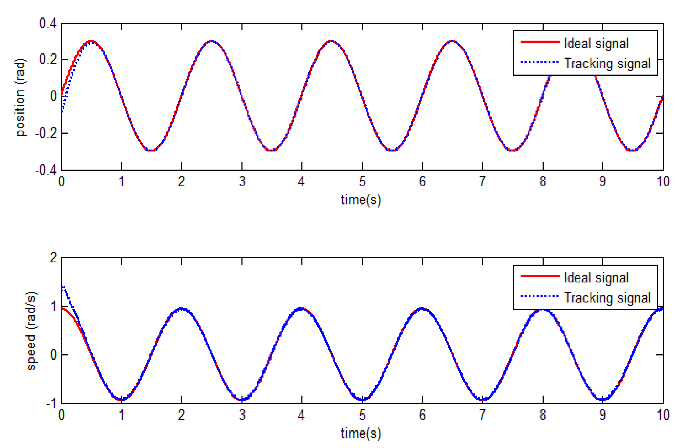
7.1. Nominal Model

Consider the dynamic equation of the ARA explained in Equation (25) of disturbance torque equal to ${\overline{\mathrm{T}}}_{\mathrm{ext}}=15\mathrm{sgn}\left({\dot{\mathsf{\Gamma }}}_{\mathrm{ra}}\right)$ and assume the initial angle and rate of angle states of the ARA are ${\overline{\mathsf{\Gamma }}}_{\mathrm{ra}}{}_{\mathrm{initial}}={\left[\begin{array}{cc}0.1& -0.11\end{array}\right]}^{\mathrm{T}}$ and ${\dot{\mathsf{\Gamma }}}_{\mathrm{ra}}{}_{\mathrm{initial}}={\left[\begin{array}{cc}0& 0\end{array}\right]}^{\mathrm{T}}$, respectively. On the other hand, it is assumed the uncertainty of the calculated dynamic model is low. Hence, the calculated mathematical dynamic model system is 0.9 of the nominal model. The required trajectory of the ARA joint 1 and joint 2 is set to ${\mathsf{\alpha }}_{1,\mathrm{d}}=0.2\sin \left(\mathsf{\pi }\mathrm{t}\right)$ and ${\mathsf{\alpha }}_{2,\mathrm{d}}=0.3\sin \left(\mathsf{\pi }\mathrm{t}\right)$, respectively. Applying the derived controller of Section 4 in equations (32, 33, 34). In this controller, the gains and parameters are set as:${ \mathrm{K}}_{\mathrm{p}}=\mathrm{diag}\left[90,90\right]$, ${\mathrm{K}}_{\mathrm{i}}=\mathrm{diag}\left[90,90\right]$,${ \mathrm{K}}_{\mathrm{\beth }}=\mathrm{diag}\left[20,20\right]$, $\mathsf{\mu }=\mathrm{diag}\left[3,3\right]$. The tracking of the position and speed of ARA joint 1 and joint 2 are presented in Figure 5 and Figure 6, respectively.

Consequently, it is shown that the controller is robust under low uncertainties. In which, ARA joint 1 and joint 2 have followed the required trajectories in definitive realization. Comparing the simulation results for the tracking trajectory in Figure 5 and Figure 6, it is obvious that ARA joint 2 is more stable and robust than ARA joint 1.

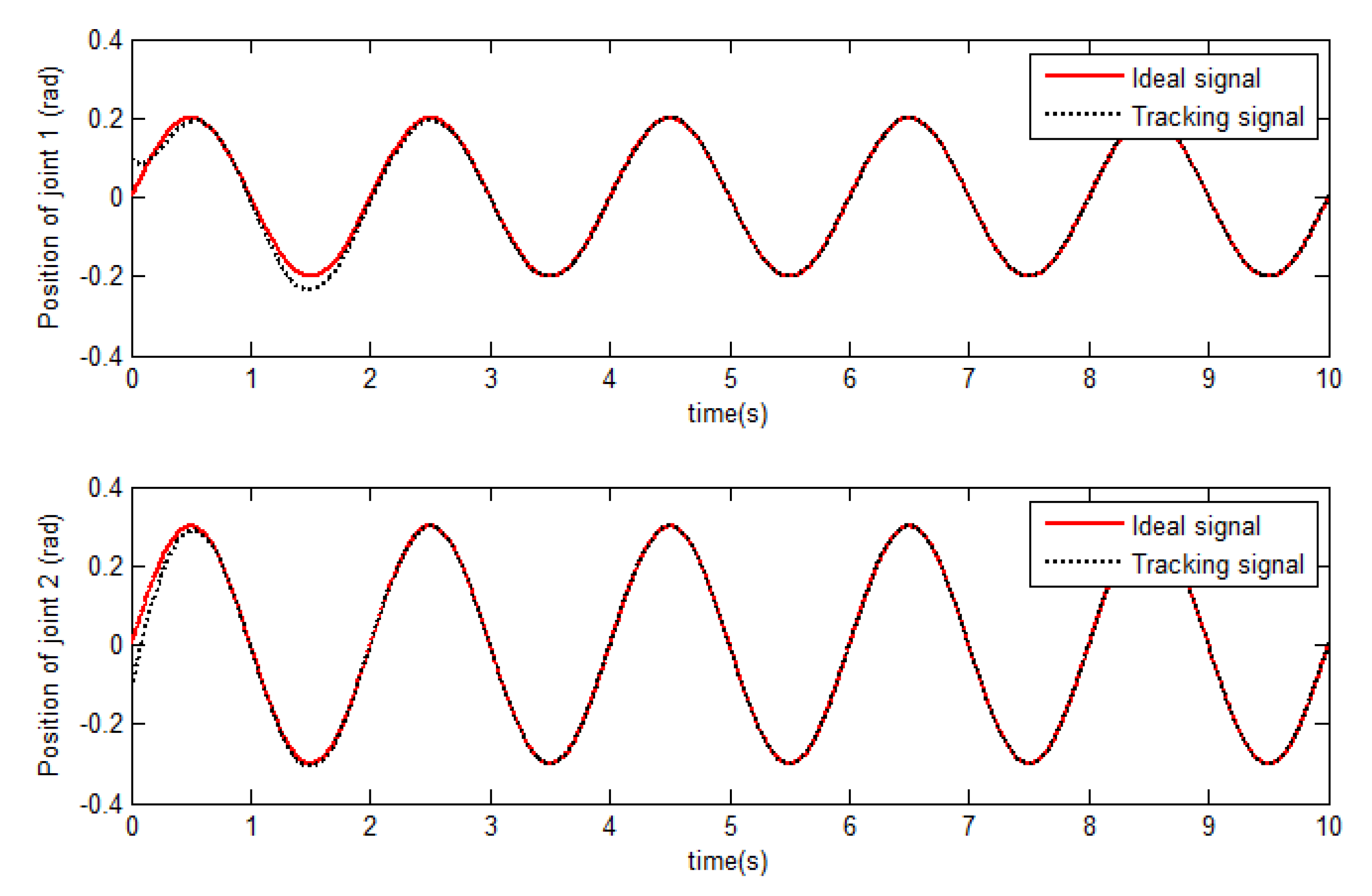
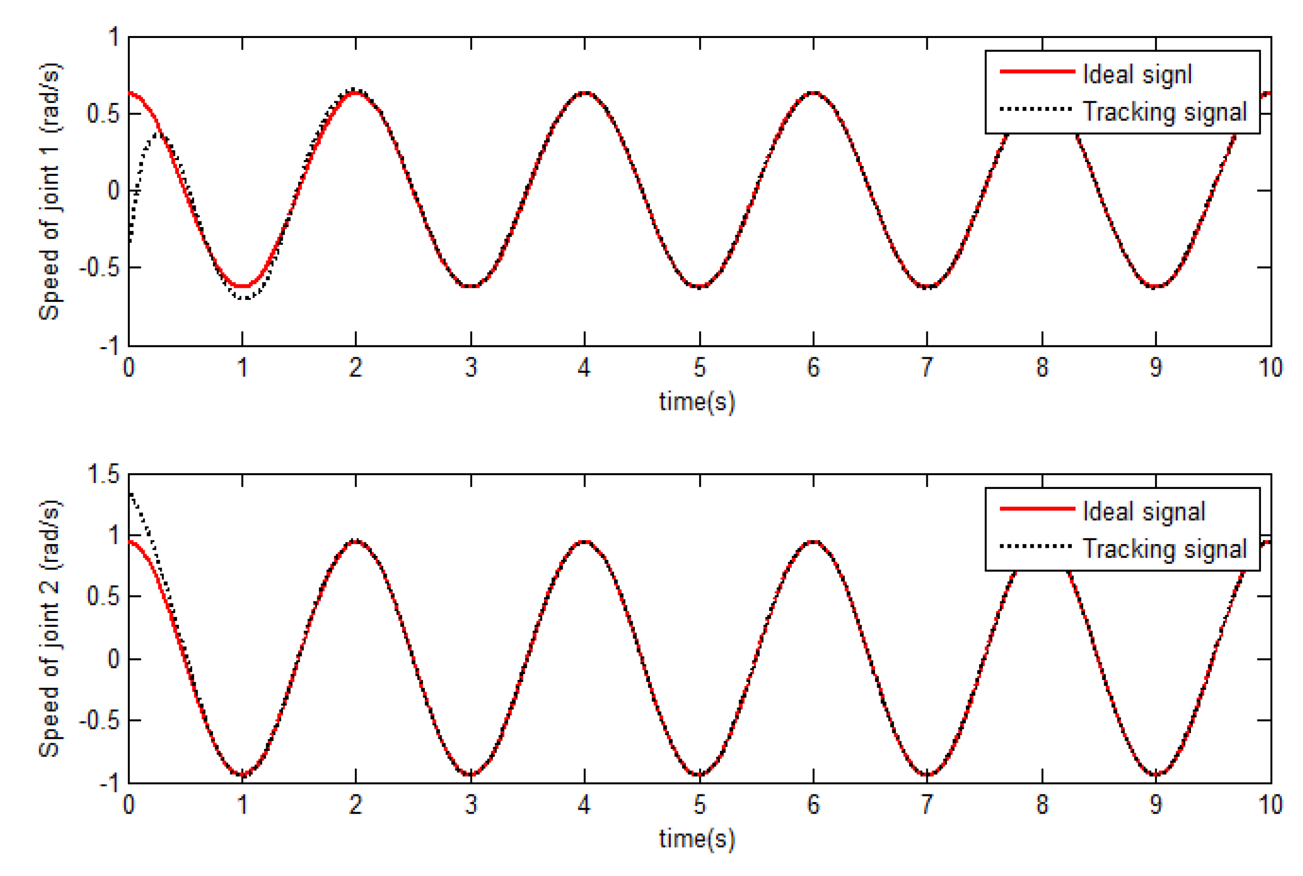
7.2. Non-Nominal Model

Assume that the ARA initial angle and rate of angle states of the ARA are ${\overline{\mathsf{\Gamma }}}_{\mathrm{ra}}{}_{\mathrm{initial}}={\left[\begin{array}{cc}0.1& -0.11\end{array}\right]}^{\mathrm{T}}$ and ${\dot{\mathsf{\Gamma }}}_{\mathrm{ra}}{}_{\mathrm{initial}}={\left[\begin{array}{cc}0& 0\end{array}\right]}^{\mathrm{T}}$, respectively. The payload of the ARA is assumed unknown and exerts a disturbance ${\overline{\mathrm{T}}}_{\mathrm{ext}}=25\mathrm{sgn}\left({\dot{\mathsf{\Gamma }}}_{\mathrm{ra}}\right)$. The required trajectory of the ARA joint 1 and joint 2 is set to ${\mathsf{\alpha }}_{1,\mathrm{d}}=0.2\sin \left(\mathsf{\pi }\mathrm{t}\right)$ ${\mathsf{\alpha }}_{2,\mathrm{d}}=0.3\sin \left(\mathsf{\pi }\mathrm{t}\right)$, respectively. Applying the derived controller of Section 5. In this controller, the gains and parameters are set as: ${\mathrm{K}}_{\mathrm{p}}=\mathrm{diag}\left[90,90\right]$, ${\mathrm{K}}_{\mathrm{i}}=\mathrm{diag}\left[90,90\right]$,${ \mathrm{K}}_{\mathrm{\beth }}=\mathrm{diag}\left[20,20\right]$, $\mathsf{\mu }=\mathrm{diag}\left[3,3\right]$. Regarding the adaptive law, the gains are assumed ${\mathrm{ᶘ}}_{{\mathrm{M}}_{\mathrm{rai}}}=6$, ${\mathrm{ᶘ}}_{{\mathrm{C}}_{\mathrm{rai}}}=13$, ${\mathrm{ᶘ}}_{{\mathrm{G}}_{\mathrm{rai}}}=7$. The structure of the RBF neural network is: the number of inputs equals 2, the number of hidden layers is 4, and the number of outputs is 1. The Gaussian function is set with the following parameters: ${\mathrm{c}}_{\mathrm{i}}=\left[\begin{array}{ccccccc}-1.3& -1.2& -0.6& 0& 0.6& 1.1& 1.6\end{array}\right]$,${ \mathrm{b}}_{\mathrm{i}}=\left[14\right]$. All the initial weights are set to zero. The uncertainty in the dynamic model of ARA is assumed to be high with the following values:

$$\begin{gathered} {\mathrm{M}}_{\mathrm{ra}}\left({\mathsf{\Gamma }}_{\mathrm{ra}}\right)=\left[\begin{array}{cc}4.8\cos \left({\mathsf{\alpha }}_2\right)& 1.9\cos \left({\mathsf{\alpha }}_2\right)\\ 1.8\cos \left({\mathsf{\alpha }}_2\right)& 0.4\end{array}\right], \\ {\mathrm{C}}_{\mathrm{ra}}=\left[\begin{array}{cc}-1.3{ \mathsf{\alpha } \dot{}}_2\sin \left({\mathsf{\alpha }}_2\right)& -1.3{ \mathsf{\alpha } \dot{}}_1\sin ({\mathsf{\alpha }}_2)\\ -1.3{ \mathsf{\alpha } \dot{}}_1\sin \left({\mathsf{\alpha }}_2\right)& 0\end{array}\right], \\ {\mathrm{G}}_{\mathrm{ra}}=\left[\begin{array}{c}39\cos \left({\mathsf{\alpha }}_1\right)+42\cos \left({\mathsf{\alpha }}_1+{\mathsf{\alpha }}_2\right)\\ 42\cos \left({\mathsf{\alpha }}_1+{\mathsf{\alpha }}_2\right)\end{array}\right]. \end{gathered}$$

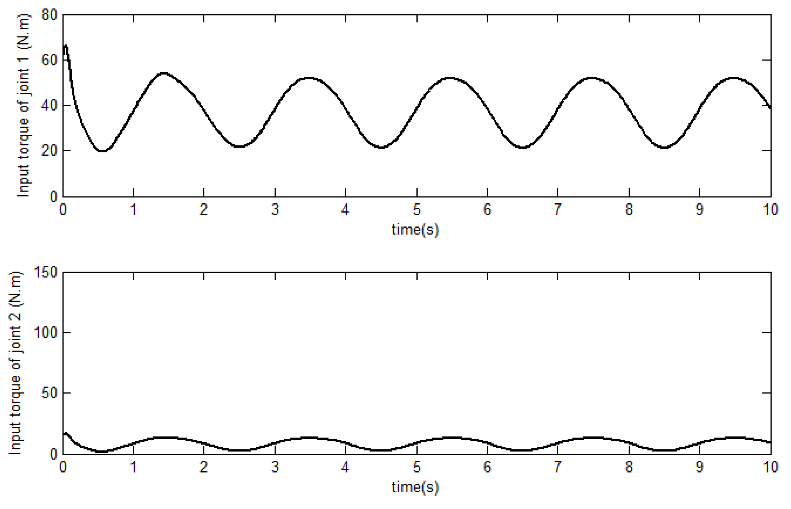
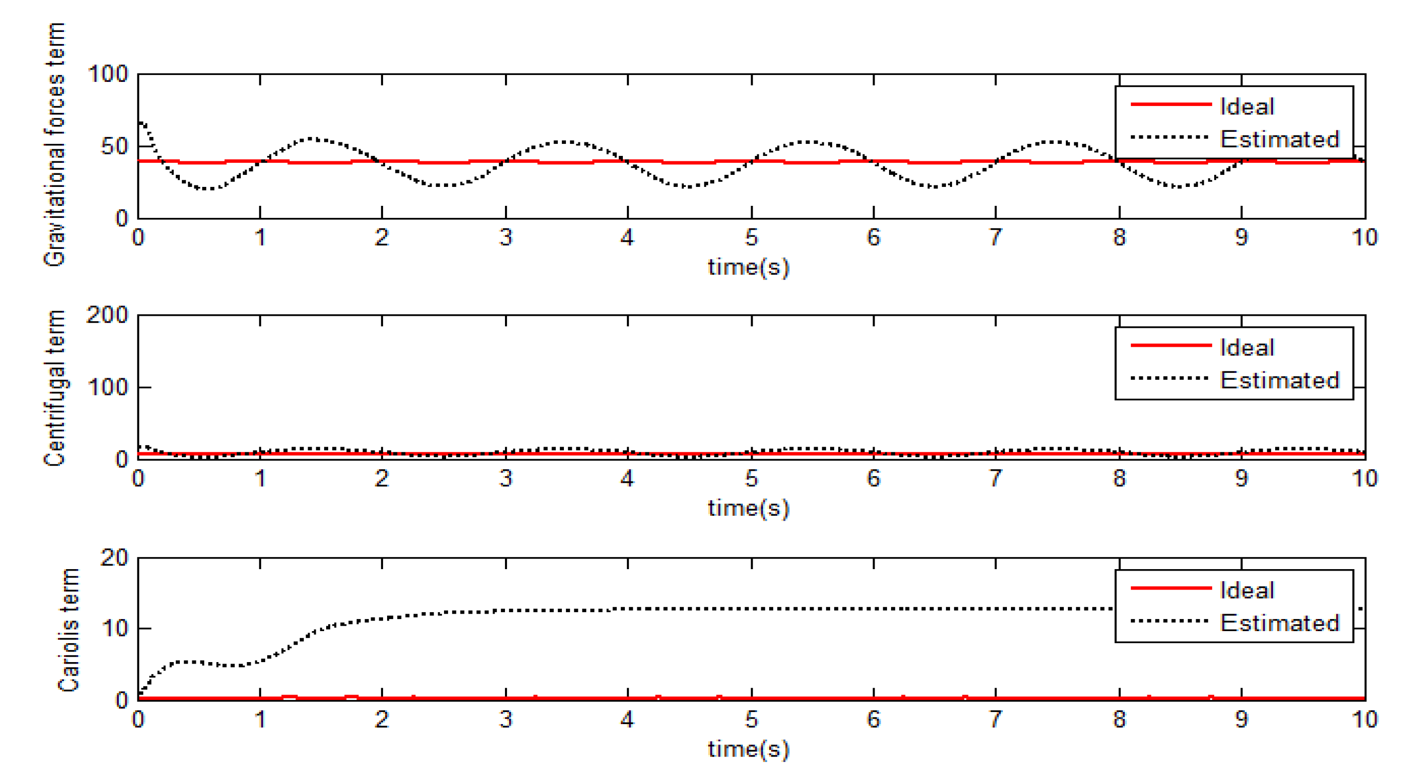
Figure 7 and Figure 8, explain the performance of the tracking trajectory of ARA joint 1 and joint 2, respectively. It is shown in these two figures, i.e., Figure 6 and Figure 7, respectively, errors of tracking in ARA joint 1 and joint 2 appear at the starting of the path before the time 2 s. Then, after time 2 s, both the required and actual trajectories are roughly overlapped. Hence, the adaptive RBF neural network control technique provides perfect tracking performances in situations where the uncertainty of the ARA dynamic is high and the payload is unknown. The required supplied torques at each ARA joint by the controller is presented in Figure 9. The required trajectory, as it existed in practical ARA manipulators, is not insistently sensational, as shown in Figure 7 and 8, respectively. Consequently, The change in the estimated terms of the dynamic system ${\hat{\mathrm{M}}}_{\mathrm{ar}}\left({\mathsf{\Gamma }}_{\mathrm{ra}}\right)$, ${\hat{\mathrm{M}}}_{\mathrm{ar}}\left({\mathsf{\Gamma }}_{\mathrm{ra}},{\dot{\mathsf{\Gamma }}}_{\mathrm{ra}}\right)$, and ${\hat{\mathrm{G}}}_{\mathrm{NN}}\left({\mathsf{\Gamma }}_{\mathrm{ra}}\right)$ presented in Figure 10 do not meet ${\mathrm{M}}_{\mathrm{ra}}\left({\mathsf{\Gamma }}_{\mathrm{ra}}\right)$, ${\mathrm{C}}_{\mathrm{ra}}\left({\mathsf{\Gamma }}_{\mathrm{ra}},{\dot{\mathsf{\Gamma }}}_{\mathrm{ra}}\right)$, and ${\mathrm{G}}_{\mathrm{ra}}\left({\mathsf{\Gamma }}_{\mathrm{ra}}\right)$, respectively.

8. Conclusions

This work presented a new controller design and simulation of an Aerial Robot Arm (ARA) that is capable of high-performing trajectory tracking under variable payload and environmental conditions. The new control algorithm takes into account high nonlinearities, coupling control loops, high modeling errors, and disturbances due to payloads and environmental conditions. The work was presented in the following steps: Firstly, a step-by-step dynamics system modeling technique for the ARA manipulator, called the Lagrange–d’Alembert principle, was introduced in detail. Then, the sliding mode algorithm was applied as a robust nominal controller. An adaptive RBF neural network was developed and applied for the robust nominal controller to handle both the high modeling errors and disturbances. Additionally, the sliding mode technique was applied to the controller, obtaining robustness to realize the required tracking execution while the RBF neural network was implemented for border-raised uncertainty. The proposed model was evaluated by two simulations. The first simulation evaluated the robustness in terms of examining the tracking trajectory of the ARA. The second simulation demonstrated the ability of the final control algorithm to stabilize and track the execution of the ARA in the presence of a high number of modeling errors and disturbances adaptively and robustly. The simulation results showed the validation and notability of the presented control algorithm. The main limitation of the proposed approach is that it does not take into account physical parameters such as the shape and texture of the object that is manipulated or moved. This can affect the overall simulation results. This issue is planned to be addressed in the future by using image recognition and depth sensors that will generate a representation of the 3D structure of the objects to be manipulated or moved. Another limitation is that the number of hidden layers and parameters of the Gaussian function could potentially affect the tracking of errors. In the future, we plan to apply an optimization technique to find the optimum RBF neural structure that will minimize the tracking errors. Additionally, alternative approaches such as deep learning networks could be applied instead of a neural network.

References

- Chen, J.; Li, S.; Liu, D.; Li, X. AiRobSim: Simulating a Multisensor Aerial Robot for Urban Search and Rescue Operation and Training. Sensors 2020, 20, 5223. [Google Scholar] [CrossRef] [PubMed]
- Liu, Y.; Gao, J.; Zhao, J.; Shi, X. A New Disaster Information Sensing Mode: Using Multi-Robot System with Air Dispersal Mode. Sensors 2018, 18, 3589. [Google Scholar] [CrossRef] [Green Version]
- Christiansen, M.P.; Laursen, M.S.; Jørgensen, R.N.; Skovsen, S.; Gislum, R. Designing and Testing a UAV Mapping System for Agricultural Field Surveying. Sensors 2017, 17, 2703. [Google Scholar] [CrossRef] [Green Version]
- Chiella, A.C.B.; Machado, H.N.; Teixeira, B.O.S.; Pereira, G.A.S. GNSS/LiDAR-Based Navigation of an Aerial Robot in Sparse Forests. Sensors 2019, 19, 4061. [Google Scholar] [CrossRef] [Green Version]
- Martinez-Martin, E.; Ferrer, E.; Vasilev, I.; del Pobil, A. The UJI Aerial Librarian Robot: A Quadcopter for Visual Library Inventory and Book Localisation. Sensors 2021, 21, 1079. [Google Scholar] [CrossRef] [PubMed]
- Feron, E.; Johnson, E.N. Aerial Robotics. In Springer Handbook of Robotics; Siciliano, B., Khatib, O., Eds.; Springer: Berlin/Heidelberg, Germany, 2008; pp. 1009–1029. [Google Scholar]
- Bulut, N.; Turgut, A.E.; Arikan, K.B. Decoupled Cascaded PID Control of an Aerial Manipulation System. Hittite J. Sci. Eng. 2019, 6, 251–259. [Google Scholar] [CrossRef] [Green Version]
- Ruggiero, F.; Lippiello, V.; Ollero, A. Aerial Manipulation: A Literature Review. IEEE Robot. Autom. Lett. 2018, 3, 1957–1964. [Google Scholar] [CrossRef] [Green Version]
- Meng, X.; He, Y.; Han, J. Survey on Aerial Manipulator: System, Modeling, and Control. Roboticac 2019, 38, 1288–1317. [Google Scholar] [CrossRef]
- Ding, X.; Guo, P.; Xu, K.; Yu, Y. A review of aerial manipulation of small-scale rotorcraft unmanned robotic systems. Chin. J. Aeronaut. 2019, 32, 200–214. [Google Scholar] [CrossRef]
- Kim, S.; Choi, S.; Kim, H.J. Aerial manipulation using a quadrotor with a two DOF robotic arm. In Proceedings of the 2013 IEEE/RSJ International Conference on Intelligent Robots and Systems, Institute of Electrical and Electronics Engineers (IEEE), Tokyo, Japan, 3–7 November 2013; pp. 4990–4995. [Google Scholar]
- Ding, L.; Wu, H. Dynamical Modelling and Robust Control for an Unmanned Aerial Robot Using Hexarotor with 2-DOF Manipulator. Int. J. Aerosp. Eng. 2019, 2019, 1–12. [Google Scholar] [CrossRef]
- Suarez, A.; Grau, P.; Heredia, G.; Ollero, A. Winged Aerial Manipulation Robot with Dual Arm and Tail. Appl. Sci. 2020, 10, 4783. [Google Scholar] [CrossRef]
- Huber, F.; Kondak, K.; Krieger, K.; Sommer, D.; Schwarzbach, M.; Laiacker, M.; Kossyk, I.; Parusel, S.; Haddadin, S.; Albu-Schaffer, A. First analysis and experiments in aerial manipulation using fully actuated redundant robot arm. In Proceedings of the 2013 IEEE/RSJ International Conference on Intelligent Robots and Systems, Institute of Electrical and Electronics Engineers (IEEE), Tokyo, Japan, 3–7 November 2013; pp. 3452–3457. [Google Scholar]
- Chermprayong, P.; Zhang, K.; Xiao, F.; Kovac, M. An Integrated Delta Manipulator for Aerial Repair: A New Aerial Robotic System. IEEE Rob. Autom Mag. 2019, 26, 54–66. [Google Scholar] [CrossRef]
- Jimenez-Cano, A.; Heredia, G.; Ollero, A. Aerial manipulator with a compliant arm for bridge inspection. In Proceedings of the 2017 International Conference on Unmanned Aircraft Systems (ICUAS), Institute of Electrical and Electronics Engineers (IEEE), Miami, FL, USA, 13–16 June 2017; pp. 1217–1222. [Google Scholar]
- Moosavian, S.A.A. Dynamics and control of free-flying robots in space: A survey. IFAC Proc. Vol. 2004, 37, 621–626. [Google Scholar] [CrossRef]
- Giordano, A.M.; Garofalo, G.; De Stefano, M.; Ott, C.; Albu-Schaffer, A. Dynamics and control of a free-floating space robot in presence of nonzero linear and angular momenta. In Proceedings of the 2016 IEEE 55th Conference on Decision and Control (CDC), Institute of Electrical and Electronics Engineers (IEEE), Las Vegas, NV, USA, 12–14 December 2016; pp. 7527–7534. [Google Scholar]
- Wang, Y.; Liang, X.; Gong, K.; Liao, Y. Kinematical Research of Free-Floating Space-Robot System at Position Level Based on Screw Theory. Int. J. Aerosp. Eng. 2019, 2019, 1–13. [Google Scholar] [CrossRef]
- Xu, S.; Wang, H.; Zhang, D.; Yang, B. Adaptive Reactionless Motion Control for Free-Floating Space Manipulators with Uncertain Kinematics and Dynamics. IFAC Proc. Vol. 2013, 46, 646–653. [Google Scholar] [CrossRef]
- Abiko, S.; Hirzinger, G. An adaptive control for a free-floating space robot by using inverted chain approach. In Proceedings of the 2007 IEEE/RSJ International Conference on Intelligent Robots and Systems, Institute of Electrical and Electronics Engineers (IEEE), San Diego, CA, USA, 29 October–2 November 2007; pp. 2236–2241. [Google Scholar]
- Xu, Y.; Gu, Y.-L.; Wu, Y.-T.; Sclabassi, R. Robust control of free-floating space robot systems. Int. J. Control. 1995, 61, 261–277. [Google Scholar] [CrossRef]
- Mital, D.P.; Leng, G.W. A voice-activated robot with artificial intelligence. Robot. Auton. Syst. 1989, 4, 339–344. [Google Scholar] [CrossRef]
- Sampedro, C.; Rodriguez-Ramos, A.; Bavle, H.; Carrio, A.; De La Puente, P.; Campoy, P. A Fully-Autonomous Aerial Robot for Search and Rescue Applications in Indoor Environments using Learning-Based Techniques. J. Intell. Robot. Syst. 2019, 95, 601–627. [Google Scholar] [CrossRef]
- Duan, H.; Shao, S.; Su, B.; Zhang, L. New development thoughts on the bio-inspired intelligence based control for unmanned combat aerial vehicle. Sci. China Ser. E Technol. Sci. 2010, 53, 2025–2031. [Google Scholar] [CrossRef]
- Tsai, L.-W. Robot Analysis: The Mechanics of Serial and Parallel Manipulators; John Wiley & Sons: New York, NY, USA, 1999; ISBN 978-0-471-32593-2. [Google Scholar]
- Schaub, H.; Junkins, J.L. Analytical Mechanics of Space Systems, 4th ed.; American Institute of Aeronautics and Astronautics: Reston, VA, USA, 2018; ISBN 978-1-62410-521-0. [Google Scholar]
- Greenwood, D.T.; Rosenberg, R.M. Classical Dynamics. J. Appl. Mech. 1977, 44, 517–518. [Google Scholar] [CrossRef] [Green Version]
- Liu, J.; Wang, X. Advanced Sliding Mode Control for Mechanical Systems; Springer: Berlin/Heidelberg, Germany, 2011. [Google Scholar]
- Alrawi, A.A.; Alobaidi, S.; Graovac, S. Robust adaptive gain for suppression of chattering in sliding mode controller. In Proceedings of the 2017 17th International Conference on Control, Automation and Systems (ICCAS), Jeju, Korea, 18–21 October 2017; pp. 951–956. [Google Scholar]
- Sands, T.; Kim, J.J.; Agrawal, B. Spacecraft Adaptive Control Evaluation. In Proceedings of the Infotech@Aerospace 2012 (American Institute of Aeronautics and Astronautics), Garden Grove, CA, USA, 19–21 June 2012; pp. 2012–2476. [Google Scholar]
- Gürlebeck, K.; Legatiuk, D.; Nilsson, H.; Smarsly, K. Conceptual modelling: Towards detecting modelling errors in engineering applications. Math. Methods Appl. Sci. 2020, 43, 1243–1252. [Google Scholar] [CrossRef]
- Liu, J. Radial Basis Function (RBF) Neural Network Control for Mechanical Systems; Springer: Berlin/Heidelberg, Germany, 2013. [Google Scholar]
- Khan, M.A.; Kim, J. Toward Developing Efficient Conv-AE-Based Intrusion Detection System Using Heterogeneous Dataset. Electronics 2020, 9, 1771. [Google Scholar] [CrossRef]
- Fu, J.-H. Lyapunov functions and stability criteria for nonlinear systems with multiple critical eigenvalues. In Proceedings of the 1992 Proceedings of the 31st IEEE Conference on Decision and Control (IEEE), Tucson, AZ, USA, 16–18 December 1992; Volume 4, pp. 3019–3024. [Google Scholar]
- Murray, R.M.; Li, Z.; Sastry, S.S. A Mathematical Introduction to Robotic Manipulation; Apple Academic Press: Waretown, FL, USA, 2017. [Google Scholar]