
Transferability of a Convolutional Neural Network (CNN) to Measure Traffic Density


Laboratory of Big-Data Applications in Public Sectors, Department of Urban Engineering, Chung-Ang University, 84 Heukseok-ro, Dongjak-gu, Seoul 156-756, Korea
*
Author to whom correspondence should be addressed.
Electronics 2021, 10(10), 1189; https://0-doi-org.brum.beds.ac.uk/10.3390/electronics10101189
Submission received: 28 April 2021
/
Revised: 11 May 2021
/
Accepted: 14 May 2021
/
Published: 16 May 2021
(This article belongs to the Special Issue AI-Based Transportation Planning and Operation, Volume II)
Abstract
:Whereas detecting individual vehicles in a video image using a convolutional neural network (CNN) prevails for traffic surveillance, CNNs also have been successfully adapted to counting vehicles via a regression method, which conveys the advantages of simplifying the model structure, and inference time can be reduced in the field. This model also demands much less human effort to tag images with labels. The number of vehicles in an image becomes the label, rather than bounding boxes drawn around every single vehicle. Nonetheless, the labeling task takes considerable time whenever a CNN model is trained and tested for a new road segment. There are two ways to alleviate the human effort involved in using this method. A previous study used a pseudo label pre-training method, and another study employed an image synthesis method to solve the problem. Besides these two methods, we investigated the model transferability to reduce the labeling effort. Using a CNN that was fully trained on images of a road segment, we devised a robust way to utilize the trained model for another site by transforming the model output with a simple quadratic equation. The utility of the proposed method was confirmed at the expense of a minute amount of deterioration in accuracy.
1. Introduction
The traffic state is represented by traffic volume, density, and space mean speed in conventional traffic theory. The relationship between the former two traffic parameters constitutes the fundamental diagram of traffic flow. The space mean speed is inversely proportional to the traffic density. The traffic volume can be computed as a product of traffic density and space mean speed. In the field of traffic engineering, measuring both the traffic density and the space mean speed is crucial to determining the level of service (LOS) of the traffic state of a road segment. The two parameters along with the traffic volume are basic indicators of the performance of traffic control and management [1]. However, a conventional space-based measurement depends on loop detectors that cannot directly measure the density and speed for a road segment.
The traffic density should be indirectly approximated from the results of a loop detector. A spot detector can measure the occupancy of a specific road segment, which indicates the ratio of the time during which vehicles occupy a detector with respect to the entire observation time, and then the density can be approximated using this occupancy based on a basic formula of traffic flow. The loop detector can measure only time mean speeds. The space mean speed also cannot be directly measured and must be estimated based on the time mean speed. Conversion errors are common, however, when using these indirect methodologies. These conversion errors typically occur either ‘from time to space’ or ‘from point to section’.
To overcome these errors, researchers often attempt to measure the traffic parameters directly from video images. Prior to the advent of the deep-learning era, many computer vision technologies were developed to address the issue. Examples include “temporal difference” [2] and “optical flow” [3,4]. Prior to the deep learning era, one of the most prevalent methodologies was referred to as “background subtraction” [5,6]. First, background subtraction extracts a base background image by averaging the pixels of an entire image sequence. Then, objects are detected within an image using the differences in the pixel values between a particular image and the base background image. This methodology, however, is vulnerable to the problem of occlusion. For example, objects such as trees or road signs can hide the vehicles in an image, at which point background subtraction cannot recognize vehicles because it regards those obstacles as repeated background.
In the post-deep-learning era, the convolutional neural network (CNN) model emerged as a newly rising technology and is responsible for a great leap forward in raising the accuracy of computer vision technologies [7]. From individual companies to large industries, many researchers have embraced this technology and developed various object detectors. Recently, CNNs have been applied to fields as diverse as the medical sciences and the autonomous vehicle industry. The “state-of-the-art” CNNs for the object detection can be categorized into two groups. Models that belong to the first category separate the region proposal task from the subsequent classification module. In the initial stage of developing these types of models, all potential regions in an image that might include an object are determined using a rule-based manner, and a learning model classifies objects for the proposed regions [8]. Both tasks were integrated to a single framework later, and region-proposal models are also trained on data to distinguish the foreground from the background [9,10]. A faster-RCNN is a two-stage model with region-proposals that has shown the best detection performance, but is handicapped by a relatively long computation time for inference.
The second category includes one-stage detection models developed to speed up the inference time at the expense of deteriorating detection accuracy. One-stage detectors simultaneously conduct both the localization and classification tasks in an end-to-end manner. The YOLO series is the most popular form of the one-stage model [11,12]. A YOLO model reduces the detection time by using a grid to divide the input image and assigning several anchor boxes to each grid for detection. An anchor box is a predefined bounding box, and its location and shape are adjusted during learning. Early versions of YOLO did not outperform the two-stage model in accuracy, but the latest version (YOLO4) has recorded equivalent, or even better, performances by reinforcing the model architecture and adopting diverse data augmentation schemes for training [13].
However, many researches who use CNNs for object detection have focused only on the problem of classification rather than regression [14,15]. Recently, CNN detectors based on the classification task have been used for traffic surveillance [16,17]. The detectors measure traffic parameters in a two-stage modeling scheme of “counting after detecting”. It is true that the method achieves the highest accuracy for traffic surveillance. However, it should be noted that deep learning-based object detectors such as YOLO [11], SSD [18], and CenterNet [19] require a great deal of human effort for the labeling task.
On the other hand, the present study uses a deep neural network as a regression model. The model simply predicts the number of vehicles in an image rather than recognizing and classifying every single vehicle. At the expense of a slight deterioration in accuracy, a regression-based CNN can simplify the model structure and drastically reduce the labeling burden compared with conventional object detectors that require the drawing of bounding boxes for all vehicles in training images. For example, it is necessary for an autonomous vehicle to detect every object and to classify them into many categories such as road, vehicle, sign, pedestrian, and so on. Even though a CNN embedded in an autonomous vehicle produces a very small error rate (=0.001%), this could lead to a serious traffic accident if only one pedestrian is not recognized. In the same context, a CNN that is used for medical diagnosis based on CT images must be error-free. However, measuring traffic parameters on a road segment does not need such high-end accuracy. The main purpose of measuring traffic states is macroscopic traffic control and management, which is non-vital. Thus, error-free detection for every vehicle on a road is redundant.
Some studies have measured road traffic parameters using CNN on a regression basis. Chung and Sohn [20] use an image as input and collectively count vehicles using a CNN. This approach achieves accuracy that is competitive against the ‘detect and count’ method, even though it is much simpler and considerably reduces the computing burden. Lee et al. [21] also measured the space mean speed based on a regression basis using two consecutive images as input. These applications are possible because measuring traffic states is “error-tolerant”. The performance, however, is much higher than that of existing loop detectors. Even before the deep learning era, there were many attempts to count pedestrians or vehicles using vision-based regression approaches [22,23]. They also recorded pretty good accuracies in the field.
Although a CNN successfully measures the traffic density and speed on a regression basis, devising a robust training method is necessary in order to apply it to many different sites. In this paper, we investigate the transferability of a CNN to measure traffic density. We sought a robust method that could use a CNN trained at a different site and transfer the data to another site without the need to retrain. Although the labeling burden for a regression-based model is much less than that of “state-of-the-art” object detectors, the objective of this study is to reduce this burden even more by utilizing the transferability of the proposed model. More concretely, the proposed approach reduced the effort that should be exerted on retraining a CNN model to collectively count vehicles whenever a site changes. A simple mathematical transformation replaced the labor-intensive re-training task.
The present paper is organized as follows. In Section 2, we briefly review our previous studies. These studies proposed two reference methods to alleviate the human effort required to tag images with labels. In Section 3, we introduce the modeling framework to adapt a CNN to a different site without training it with a large labeled dataset. More concretely, we propose how to utilize a nonlinear transformation methodology to transfer a CNN output to other sites, and the performance of the transferred output is compared with that from a fine-tuned model. In Section 4, five different augmentation schemes are applied to images of the target road segment to test how well the model can be transferred to various conditions. For the augmentation, original images are scaled, rotated, and flipped. In the last section, we draw conclusions and suggest future tasks that are beyond the scope of this study.
2. Reviewing Our Previous Effort to Alleviate the Labeling Burden
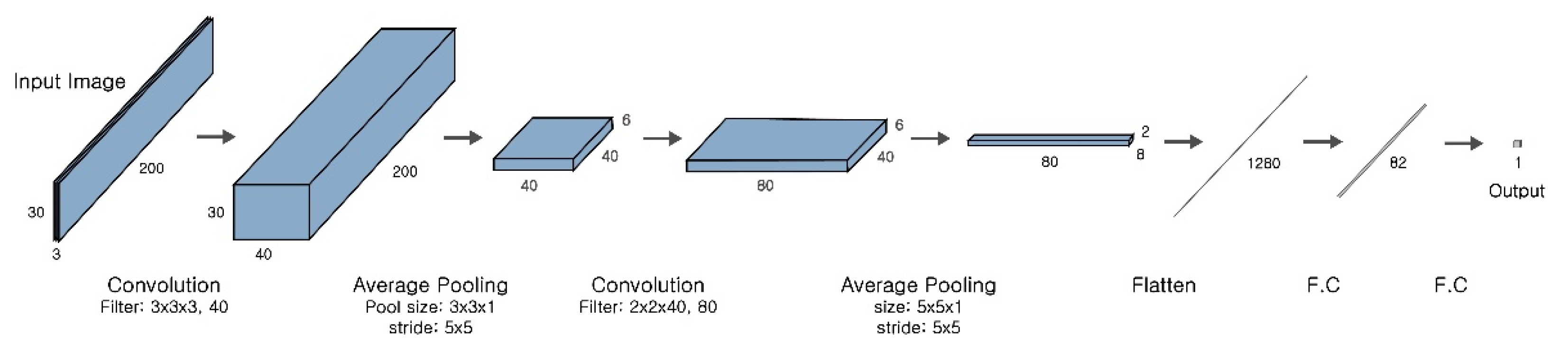
The proposed transferability study of the CNN model builds upon our two previous studies [20,21]. First, a brief description of the CNN model proposed in our first reference study [20] follows. In the initial stage, video images to train and test the CNN model were collected and adjusted. We collected 6 h and 26 min of video stream for an intersection located in Seoul, South Korea. From the video frames, we randomly chose 23,164 images. We cropped a 145 m length approach from the intersection, and with a simple rotating and resizing process, we were able to obtain standardized rectangular images (200 × 30 pixels). The preprocessed images served as input for the proposed CNN model. The preprocessed images were randomly separated into 20% testing data (=4632 images) and 80% training data (=18,532 images). In order to reflect various weather conditions, data augmentation schemes were applied to the training data. Five different image filters were used to sharpen and blur the training images, which increased the number of training images to 111,192. In summary, the mean absolute error (MAE) ranged from 1.34~1.57. The result was very encouraging considering the number of vehicles in an image averaged 53.2.
The background subtraction method was far less accurate than the proposed CNN. However, that method requires no human effort, because it does not require labeling. To label an image for training and testing a CNN, the number of vehicles in the image must be manually counted. Overall, more than 1.15 million cars in 23,164 images were counted. This huge consumption of time and effort could be a barrier to application of the CNN method to other sites. The previous study suggested an approach to reduce the labeling burden by using the pseudo labels achieved from the background subtraction method. First, a CNN model was pretrained with a pseudo label and fine-tuned with a small amount of labeled images. However, at least 20% of the training data (3706 = 18,532 × 0.2) was necessary to acquire an acceptable level of accuracy, which was also burdensome.
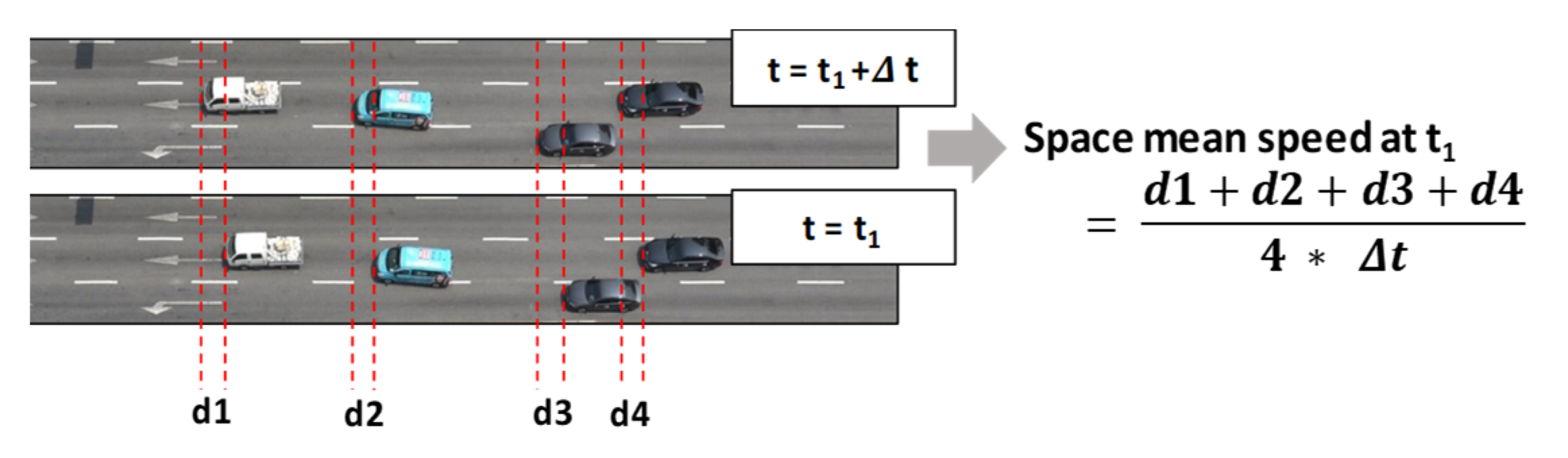
The second previous study also used a CNN as a regression model to measure the space mean speed on a road segment [21]. The CNN was fed by two consecutive images taken in a very short time (=0.1 s). Capturing the displacement of a vehicle’s position between two consecutive images was a key to deriving the space mean speed (see Figure 1). None of the detectors available before the deep-learning era have succeeded in directly measuring this speed. Our previous study was the first attempt to use a CNN to measure the space mean speed on a road segment. As the results from the study show, it was very promising to measure the speed based on a CNN fed by two consecutive video images.
Utilizing the proposed CNN model in the field, however, was a big challenge. The labeling task for the model is much harder than that for the CNN when measuring traffic density. The space mean speed can be computed from the average of displacements made by all vehicles between two consecutive images. Manually measuring the distances is a formidable task. The previous study suggested a plausible way to overcome the complication. That study focused on a generative adversary net (GAN) to synthesize a large amount of labeled images [24]. In particular, a cycle-consistent adversarial network (CycleGAN) that transforms images between two different domains was employed to secure pseudo-labeled images [25].
More concretely, unpaired sets of animation and real photo images are used to train a CycleGAN, and the trained model converts animation images into believable imitation versions. The synthesized images contain a full amount of traffic information that can be used as labels, as it originates from a traffic simulation. Figure 2 shows an example pair of the two images. Although this method required fine-tuning after training using the synthesized images, the amount of manually labeled images was much smaller than that of the background subtraction method adopted in the first reference study to measure traffic density.
Despite the success of measuring the space mean speed based on a CNN trained on synthesized images, an additional engineering task is necessary for the method. Believable synthesized images should be obtained from a well-established simulation environment. To do so, the traffic and road geometric conditions of a target site should be identified in advance, so that a simulated environment that mimics the real state can be set up. Once such conditions are identified, animation images that the simulation program provides can be directly used to synthesize labeled images for the measurement. This procedure demands expertise in traffic engineering, which may be a different type of limitation.
After reviewing the two previous attempts to alleviate the labeling burden, we realized that a more robust and simpler approach is necessary to reuse a model for different sites without much human effort for the labeling task. As a result, a novel approach based on a simple mathematical transformation was developed, and the test results of the performance in measuring traffic density are reviewed in what follows.
3. Modeling Framework to Transfer a Trained CNN to Another Site
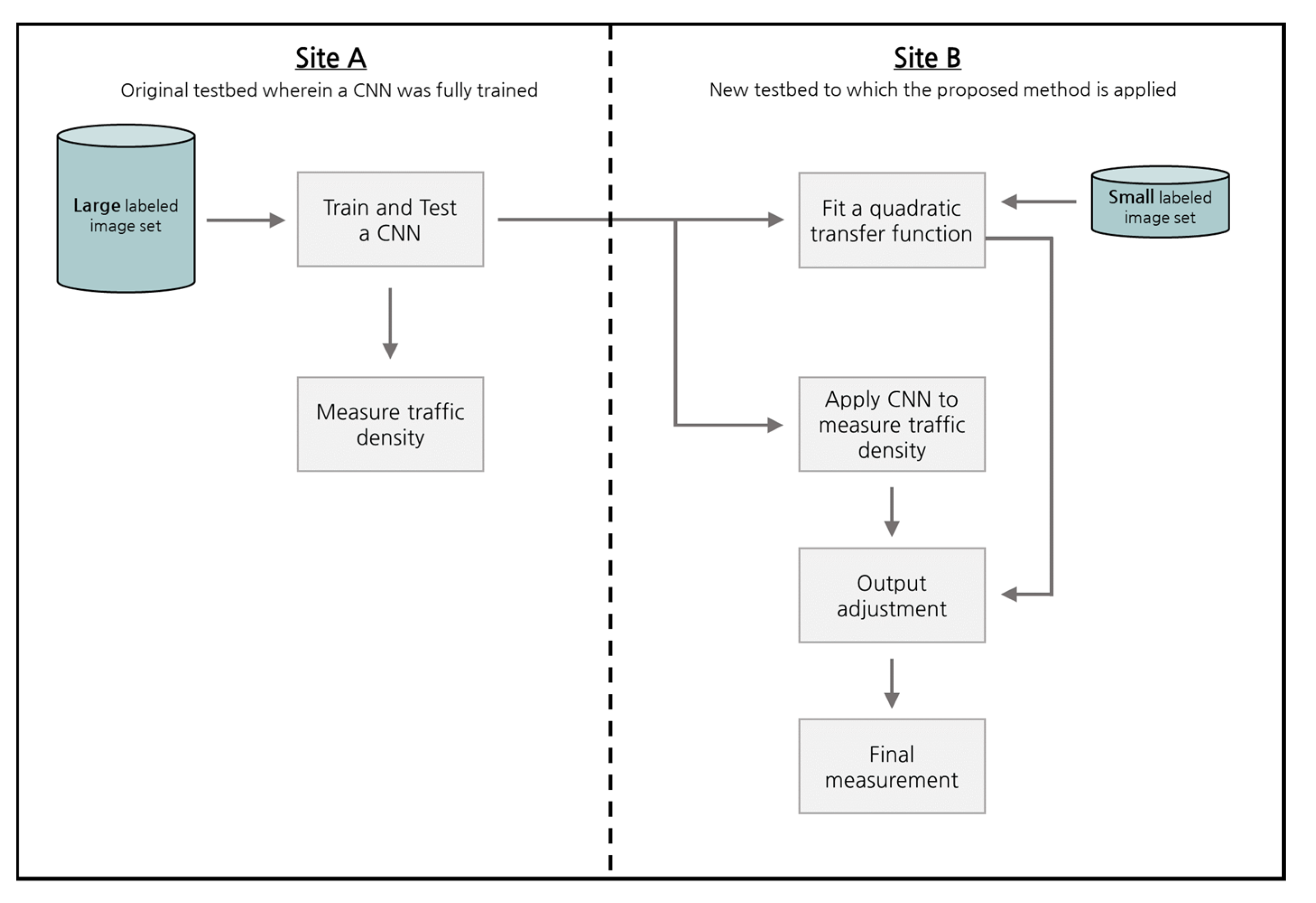
In this section, we test the transferability of a CNN and introduce a methodology to increase its performance in measuring traffic density in a new road segment without additional training. The structure of this CNN is the same as that in our previous study [20], as shown in Figure 3. An image of a road segment where vehicles are to be counted feeds the model, and the model returns a single real number that corresponds to the vehicle count. Once a vehicle count is obtained, the corresponding traffic density is automatically measured by dividing it by the length of the road segment. For this reason, the two terms ‘vehicle count’ and ‘traffic density’ are interchangeably used in this paper. To measure traffic density in a newly chosen road segment, the previously trained model was used without further training to count vehicles. This method avoids huge amounts of time and effort for labeling, but there is no guarantee that the same high measurement level of accuracy will be obtained as in the original site. Therefore, we had to consider the model transferability. In this section, we describe testing the model transferability using the model that was already trained in the previous study [20]. The modeling procedure of transferring a CNN to a new site is shown in Figure 4.
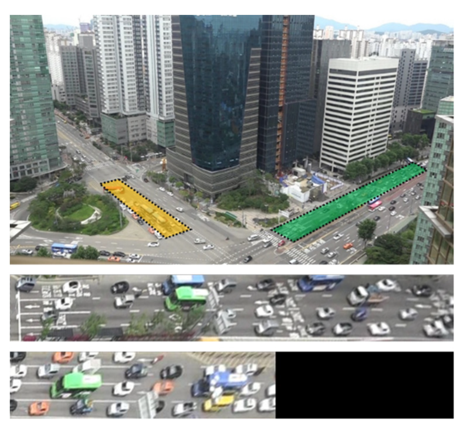
To test the model transferability, we used the same video clip from the previous study [20]. This time, however, we cropped another approach in the 10 o’clock direction, which is depicted as a yellow square in Figure 5. We have a total of 23,164 snapshot images (1 frame per second), but this time, we randomly chose only 600 images because of the difficulty of labeling. The numbers were smaller than the fine-tuning in the CNN models in the two previous studies. Afterwards, only 500 images were used to estimate the transformation equation and the remaining 100 images were reserved for test. To apply the previously trained CNN model to other road segments, the same input size should be maintained. The length of the new road segment was shorter than the former one, so we performed zero padding on the remaining part of the image. The new road segment had a 120 × 30 pixel size, so to achieve a 200 × 30 input size, we attached (0, 0, 0) RGB values to the last 80 × 30 pixels. Figure 5 shows the converted sample image for the newly chosen road segment.
The previously trained CNN model was used to predict the number of vehicles in the new road segment. We tested this model on 100 test images and compared the test results with the former test results from the original site. Table 1 lists the performance indices that were used to compare the measurement accuracy. The first column (A) represents the test results when the previously trained model was applied to the original road segment, and the second column (B) represents the test results when the model was applied to the newly added road segment. The horizontal axes of the plots in the table denote the actual counts of vehicles, and the vertical axes denote the predicted number of vehicles. As expected, the measurement error for (B) was larger than that for (A). The mean absolute error (MAE) for the new road segment was almost 10 times higher than the previous measurement at the original site.
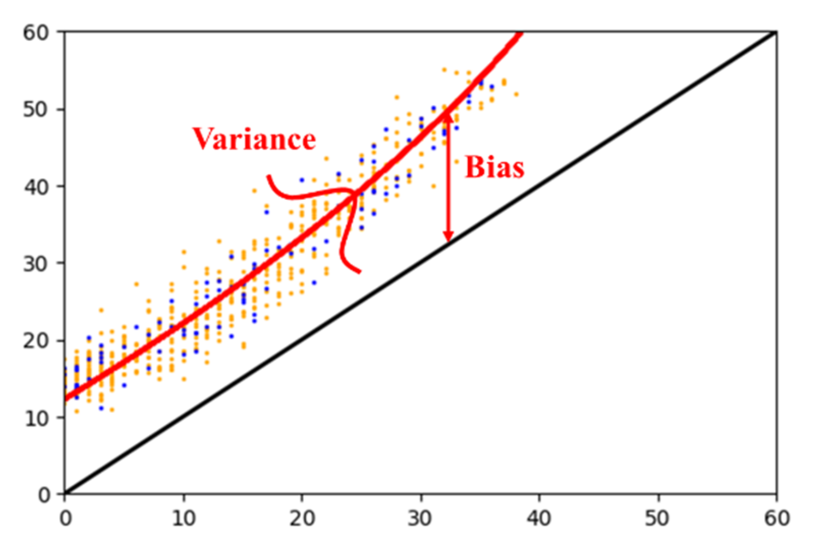
The interesting point is, however, that in the newly chosen site (B), the correlation coefficient between observed and estimated vehicle counts remains very close to one. This finding offered the possibility that there could be a constant relationship between a real label and that predicted by the earlier trained model. From this observation, we attempted to find a simple nonlinear transformation equation to account for the relationship. To find the equation, a small number of labeled images was necessary for the new road segment. With only 500 training data points (=labeled images), we solved the curve-fitting problem and estimated a simple quadratic equation, as shown in Figure 6. The data points have both a bias and a variance. If the equation moves the data from the regression line to the identity line (a set of points that shows the predict label is the real label, y = x), the bias can be removed, but the variance remains.
The nonlinear data transformation procedure is quite simple. Each image out of the newly chosen 500 images has two labels that are predicted by a trained CNN model and a real label. A quadratic equation for the population regression line was set up in Equation (1).
In Equation (1), denotes a real label, denotes the predicted label, ( are parameters to be estimated, and is a random term that is assumed to be distributed by a Gaussian distribution with a zero mean. The three parameters of this regression equation were estimated using the 500 data points. Equation (2) shows the sample regression line after implementing the least square estimation.
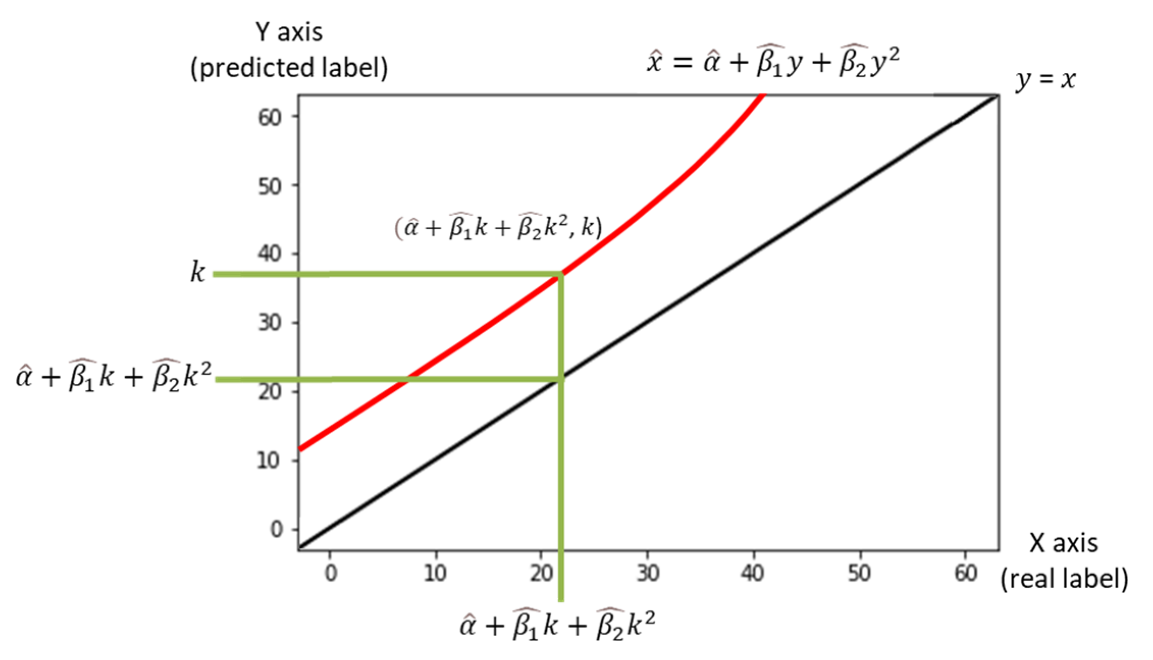
In Equation (2), is an estimate of , and ( are estimates for (. To adjust the number () predicted by the CNN into a more plausible estimate, the number () should be projected on the transformation equation and becomes . The projected number then bridges the gap between the number predicted by the CNN and the final estimate. Figure 7 visualizes the relationship. Every image (=data point) has a coordinate in the 2D plain [real label, predicted label] in Figure 6. We can express each image using the predicted number () and the corresponding estimated number [,]. For further explanation, the data point can be regarded as moving into [, ].
As mentioned earlier, even though the bias is clearly removed, the variance remains and has a negative effect on the measurement accuracy. However, this methodology has an advantage in computational efficiency. Calibrating the regression equation took just 0.002 s when using 500 images. For comparison, the previously trained CNN model was fine-tuned using the 500 labeled images. In this fine-tuning, the weights of the previously trained CNN model were adopted as the initial values. The results appear in Table 2. As expected, the fine-tuned CNN exhibited a slightly better performance. However, additional training time for the fine-tuning was almost 277,000 times longer than implementing the proposed nonlinear transformation scheme. This result supports our objective to develop a simple transfer method to use a CNN model to measure traffic density without retraining.
4. Testing for Varying Ambient Conditions of a Road Segment
The proposed methodology should be tested for various conditions of road segments. Unfortunately, preparing labeled images for additional sites requires considerable cost and effort. Thus, to test the proposed methodology under various conditions, we synthesized several images by augmenting images of the newly selected road segment. The first image in Table 3 is the road segment chosen in our previous study, wherein a full dataset was collected and the CNN model was trained on them. The second image is a baseline (Case 1) that shows the real conditions of the newly chosen road segment. For testing the model transferability, we synthesized additional images by distorting the baseline image. In Case 2, a new image was created by shrinking the baseline image. In Case 3, we stretched the baseline image from side to side. Case 4 rotates the scaled image of Case 2. At last, a flipped image of the baseline image was included in Case 5.
Table 3 lists the test results from the cases of different road conditions reflected by synthesized images. The margin of the images was zero-padded with a black border. For each case of the newly chosen road segment, three different approaches were tested. First, the model trained on the baseline images was applied to each case, which is titled naïve prediction (D). The second approach (E) denotes the proposed quadratic transformation method, and the third approach (F) represents the fine-tuning of the previous CNN.
For comparison, the same 100 test images were used. Because of the shorter length of the new road segment, the mean of the vehicle counts was lower than that of the reference case, so %RMSE appeared to be a bit high. However, the MAE maintained the same level as the reference case for the approach based on the fine-tuned CNN model (F). Regarding the computation efficiency, the nonlinear transformation methodology (E) required only 0.002~0.003 s for all cases. If an MAE of 1.0–1.5 was tolerable, it would be acceptable in the field. An interesting point of the experiment is that the performance gap between the proposed approach (E) and the fine-tuning approach (F) was decreased when the resolution of the images deteriorated (Case 3). That is, the proposed transformation approach would be promising where obtaining high-resolution images is difficult, which is common in real traffic surveillance systems that depend on CCTVs.
5. Conclusions
The present study set up a simple CNN model and trained it elaborately using data augmentation skills. The model achieved very good performance in measuring traffic density. Training the CNN for a new site, however, requires a large amount of both human effort and computing resources. We reused an already trained CNN model in a new road segment without fine-tuning based on newly labeled data, and only 500 training images were used to transform the naïve output returned by the model into a result closer to the ground truth.
A nonlinear data transformation methodology was developed and was competitive against the fine-tuning approach. The methodology also recorded the shortest computing time (=0.002 s). If we must apply our density measure methodology to many road segments, the nonlinear transformation methodology would be advantageous.
There are some limitations in the present study. First, we tested five different cases using augmented images attained from just one approach. In further study, we will perform tests on as many different locations as possible. In addition, we took the video only during the daytime where no dramatic changes occur. More tests should be carried out on various conditions in the future. Second, we trained the baseline CNN model on 18,532 images. It is well known that a larger amount of training data produces a better result. A dataset that is too large, however, diminishes the efficiency of computation. We should perform sensitivity analysis to establish the proper size for training data. In addition, we had no systematic way to choose the hyperparameters of the baseline CNN, which necessitated many trials.
Author Contributions
Conceptualization, K.S.; Software and Data curation, J.C. and G.K.; Writing-Original draft preparation, J.C.; Investigation and Visualization, G.K.; Methodology, Writing-Reviewing and Editing, K.S. All authors have read and agreed to the published version of the manuscript.
Funding
This research was supported by the Chung-Ang University Research Scholarship Grants in 2019; in part by the National Research Foundation of Korea (NRF) Grant funded by the Korean Government (2021R1A2C2003842); and in part by the Korea Agency for Infrastructure Technology Advancement (KAIA) grant funded by the Ministry of Land, Infrastructure, and Transport (Grant21TLRP-B148677-04).
Data Availability Statement
The data presented in this study are available in [https://00bigdata.cau.ac.kr] (accessed on 16 April 2021).
Conflicts of Interest
The authors declare no conflict of interest.
References
- Ryus, P.; Vandehey, M.; Elefteriadou, L.; Dowling, R.G.; Ostrom, B.K. Highway Capacity Manual 2010; Transportation Research Board: Washington, DC, USA, 2010. [Google Scholar]
- López, M.T.; Fernández-Caballero, A.; Mira, J.; Delgado, A.E.; Fernández, M.A. Algorithmic lateral inhibition method in dynamic and selective visual attention task: Application to moving objects detection and labeling. Expert. Syst. Appl. 2006, 31, 570–594. [Google Scholar] [CrossRef] [Green Version]
- López, M.T.; Fernández-Caballero, A.; Fernández, M.A.; Mira, J.; Delgado, A.E. Visual Surveillance by Dynamic Visual Attention Method. Pattern Recogn. 2006, 39, 2194–2211. [Google Scholar] [CrossRef] [Green Version]
- Ji, X.; Wei, Z.; Feng, Y. Effective vehicle detection technique for traffic surveillance systems. J. Vis. Commun. Image Represent. 2006, 17, 647–658. [Google Scholar] [CrossRef]
- Zhou, J.; Gao, D.; Zhang, D. Moving vehicle detection for automatic traffic monitoring. IEEE Trans. Veh. Technol. 2007, 56, 51–59. [Google Scholar] [CrossRef] [Green Version]
- Niu, X. A semi-automatic framework for highway extraction and vehicle detection based on a geometric deformable model. ISPRS J. Photogramm. Remote Sens. 2006, 61, 170–186. [Google Scholar] [CrossRef]
- Krizhevsky, A.; Sutskever, I.; Hinton, G.E. ImageNet classification with deep convolutional neural networks. Adv. Neural Inf. Process. Syst. 2012, 25, 1097–1105. [Google Scholar] [CrossRef]
- Girshick, R.; Donahue, J.; Darrell, T.; Malik, J. Rich feature hierarchies for accurate object detection and semantic segmentation. In Proceedings of the IEEE Conference on Computer Vision and Pattern Recognition, Columbus, OH, USA, 23–28 June 2014; pp. 580–587. [Google Scholar]
- Girshick, R. Fast r-cnn. In Proceedings of the IEEE International Conference on Computer Vision, Santiago, Chile, 7–13 December 2015; pp. 1440–1448. [Google Scholar]
- Ren, S.; He, K.; Girshick, R.; Sun, J. Faster R-CNN: Towards real-time object detection with region proposal networks. IEEE Trans. Pattern Anal. Mach. Intell. 2016, 39, 1137–1149. [Google Scholar] [CrossRef] [PubMed] [Green Version]
- Redmon, J.; Divvala, S.; Girshick, R.; Farhadi, A. You only look once: Unified, real-time object detection. In Proceedings of the IEEE Conference on Computer Vision and Pattern Recognition, Las Vegas, NV, USA, 27–30 June 2016; pp. 779–788. [Google Scholar]
- Redmon, J.; Farhadi, A. Yolov3: An incremental improvement. arXiv 2018, arXiv:1804.02767. [Google Scholar]
- Bochkovskiy, A.; Wang, C.Y.; Liao, H.Y.M. Yolov4: Optimal speed and accuracy of object detection. arXiv 2020, arXiv:2004.10934. [Google Scholar]
- Messelodi, S.; Modena, C.M.; Zanin, M. A computer vision system for the detection and classification of vehicles at urban road intersections. Pattern Anal. Appl. 2005, 8, 17–31. [Google Scholar] [CrossRef]
- Park, K.; Lee, D.; Park, Y. Video-based detection of street-parking violation. In Proceedings of the International Conference on Image Processing, Computer Vision, and Pattern Recognition (IPCV), Las Vegas, NV, USA, 25–28 June 2007; Volume 1, pp. 152–156. [Google Scholar]
- Sommer, L.W.; Schuchert, T.; Beyerer, J. Fast deep vehicle detection in aerial images. In Proceedings of the IEEE Winter Conference on Applications of Computer Vision (WACV), Santa Rosa, CA, USA, 24 March 2017; pp. 311–319. [Google Scholar]
- Wang, L.; Lu, Y.; Wang, H.; Zheng, Y.; Ye, H.; Xue, X. Evolving boxes for fast vehicle detection. In Proceedings of the IEEE International Conference on Multimedia and Expo, Hong Kong, China, 10–14 July 2017; pp. 1135–1140. [Google Scholar]
- Liu, W.; Anguelov, D.; Erhan, D.; Szegedy, C.; Reed, S.; Fu, C.Y.; Berg, A.C. Ssd: Single shot multibox detector. In Proceedings of the European Conference on Computer Vision, Amsterdam, The Netherlands, 8–16 October 2016; pp. 21–37. [Google Scholar]
- Zhou, X.; Wang, D.; Krähenbühl, P. Objects as points. arXiv 2019, arXiv:1904.07850. [Google Scholar]
- Chung, J.; Sohn, K. Image-Based Learning to Measure Traffic Density Using a Deep Convolutional Neural Network. IEEE Trans. Intell. Transp. Syst. 2018, 19, 1670–1675. [Google Scholar] [CrossRef]
- Lee, J.; Roh, S.; Shin, J.; Sohn, K. Image-based learning to measure the space mean speed on a stretch of road without the need to tag images with labels. Sensors 2019, 19, 1227. [Google Scholar] [CrossRef] [PubMed] [Green Version]
- Chen, K.; Gong, S.; Xiang, T.; Loy, C.C. Cumulative attribute space for age and crowd density estimation. In Proceedings of the IEEE Conference on Computer Vision and Pattern Recognition (CVPR), Portland, OR, USA, 23–28 June 2013; pp. 2467–2474. [Google Scholar]
- Zhang, C.; Li, H.; Wang, X.; Yang, X. Cross-scene crowd counting via deep convolutional neural networks. In Proceedings of the IEEE Conference on Computer Vision and Pattern Recognition (CVPR), Boston, MA, USA, 7–12 June 2015; pp. 833–841. [Google Scholar]
- Goodfellow, I.; Pouget-Abadie, J.; Mirza, M.; Xu, B.; Warde-Farley, D.; Ozair, S.; Bengio, Y. Generative adversarial nets. In Proceedings of the Conference on Advances in Neural Information Processing Systems, Montreal, QC, Canada, 8–13 December 2014; pp. 2672–2680. [Google Scholar]
- Zhu, J.Y.; Park, T.; Isola, P.; Efros, A.A. Unpaired image-to-image translation using cycle-consistent adversarial networks. In Proceedings of the IEEE International Conference on Computer Vision, Venice, Italy, 22–29 October 2017; pp. 2223–2232. [Google Scholar]
Figure 1.
Conceptual explanation of space mean speed [21].
Figure 1.
Conceptual explanation of space mean speed [21].

Figure 2.
An example of converting a simple naïve image into a believable synthesized image.

Figure 3.
Convolutional neural network (CNN) model architecture.

Figure 4.
Modeling framework to transfer a CNN to another site.

Figure 5.
The original video snapshot (top), the green approach to train the former CNN model (middle), and the new yellow approach to test the transferability of the trained model (bottom). The new approach is zero-padded.
Figure 5.
The original video snapshot (top), the green approach to train the former CNN model (middle), and the new yellow approach to test the transferability of the trained model (bottom). The new approach is zero-padded.

Figure 6.
Every data point has a variance and a bias. The bias can be removed using the nonlinear data transformation.
Figure 6.
Every data point has a variance and a bias. The bias can be removed using the nonlinear data transformation.

Figure 7.
Transformation of the original estimate into the final estimate.


Table 1.
Results of the naïve prediction for the new approach. RMSE, root mean square error; MAE, mean absolute error.
Table 1.
Results of the naïve prediction for the new approach. RMSE, root mean square error; MAE, mean absolute error.
| Test Result on the Original Road Segement (A) | Naïve Predict on New Road Segement (B) | |
|---|---|---|
| Plot |  |  |
| Number of test data | 4632 | 100 |
| %RMSE | 3.4920 | 90.283 |
| MAE | 1.3427 | 13.586 |
| Correlation coefficient | 0.995 | 0.967 |
Table 2.
Comparison of data transformation and convolutional neural network (CNN) training for a new approach.
Table 2.
Comparison of data transformation and convolutional neural network (CNN) training for a new approach.
| Nonlinear Transformation | CNN Finetuning | |
|---|---|---|
| Plot |  |  |
| Number of test data | 100 | 100 |
| %RMSE | 17.002 | 11.255 |
| MAE | 2.125 | 1.271 |
| Correlation coefficient | 0.970 | 0.991 |
| Additional training time | 0.002 s | 554.477 s |
Table 3.
Model performance for various augmented conditions.
Reference case (Image of the previous road segment) | ||||
| Test result | %RMSE | MAE | Corr. Coeff. | Additional training |
| 3.492 | 1.343 | 0.995 | 0.000 s | |
Case 1 (Baseline: original image of the newly chosen road segment) | ||||
| %RMSE | MAE | Corr. Coeff. | Additional training | |
| Naïve prediction (D) | 90.283 | 13.586 | 0.967 | 0.000 s |
| Nonlinear data transformation (E) | 17.002 | 2.125 | 0.970 | 0.002 s |
| CNN finetuning (F) | 11.255 | 1.271 | 0.991 | 554.477 s |
Case 2 (Downsized image) | ||||
| %RMSE | MAE | Corr. Coeff. | Additional training | |
| Naïve prediction (D) | 64.482 | 8.160 | 0.943 | 0.000 s |
| Nonlinear data transformation (E) | 22.774 | 2.834 | 0.946 | 0.002 s |
| CNN finetuning (F) | 10.995 | 1.279 | 0.989 | 600.439 s |
Case 3 (Upscaled image) | ||||
| %RMSE | MAE | Corr. Coeff. | Additional training | |
| Naïve prediction (D) | 37.056 | 4.383 | 0.972 | 0.000 s |
| Nonlinear data transformation (E) | 15.984 | 2.071 | 0.975 | 0.003 s |
| CNN finetuning (F) | 12.944 | 1.596 | 0.987 | 856.122 s |
Case 4 (Downsized and rotated image) | ||||
| %RMSE | MAE | Corr. Coeff. | Additional training | |
| Naïve prediction (D) | 33.038 | 4.355 | 0.951 | 0.000 s |
| Nonlinear data transformation (E) | 21.249 | 2.672 | 0.953 | 0.001 s |
| CNN finetuning (F) | 11.810 | 1.437 | 0.989 | 675.667 s |
Case 5 (Flipped image) | ||||
| %RMSE | MAE | Corr. Coeff. | Additional training | |
| Naïve prediction (D) | 95.239 | 13.998 | 0.937 | 0.000 s |
| Nonlinear data transformation (E) | 22.228 | 2.668 | 0.949 | 0.003 s |
| CNN finetuning (F) | 12.584 | 1.547 | 0.986 | 674.942 s |
Publisher’s Note: MDPI stays neutral with regard to jurisdictional claims in published maps and institutional affiliations. |
© 2021 by the authors. Licensee MDPI, Basel, Switzerland. This article is an open access article distributed under the terms and conditions of the Creative Commons Attribution (CC BY) license (https://creativecommons.org/licenses/by/4.0/).
Share and Cite
MDPI and ACS Style
Chung, J.; Kim, G.; Sohn, K. Transferability of a Convolutional Neural Network (CNN) to Measure Traffic Density. Electronics 2021, 10, 1189. https://0-doi-org.brum.beds.ac.uk/10.3390/electronics10101189
AMA Style
Chung J, Kim G, Sohn K. Transferability of a Convolutional Neural Network (CNN) to Measure Traffic Density. Electronics. 2021; 10(10):1189. https://0-doi-org.brum.beds.ac.uk/10.3390/electronics10101189
Chicago/Turabian StyleChung, Jiyong, Gyeongjun Kim, and Keemin Sohn. 2021. "Transferability of a Convolutional Neural Network (CNN) to Measure Traffic Density" Electronics 10, no. 10: 1189. https://0-doi-org.brum.beds.ac.uk/10.3390/electronics10101189
Note that from the first issue of 2016, this journal uses article numbers instead of page numbers. See further details here.