A Review of I–V Tracers for Photovoltaic Modules: Topologies and Challenges

Abstract

Current–voltage (I–V) curve tracers are used for measuring voltage and current in photovoltaic (PV) modules. I–V curves allow identifying certain faults in the photovoltaic module, as well as quantifying the power performance of the device. I–V curve tracers are present in different topologies and configurations, by means of rheostats, capacitive loads, electronic loads, transistors, or by means of DC–DC converters. This article focuses on presenting all these configurations. The paper shows the electrical parameters to which the electronic elements of the equipment are exposed using LTSpice, facilitating the appropriate topology selection. Additionally, a comparison has been included between the different I–V tracers’ topologies, analyzing their advantages and disadvantages, considering different factors such as their flexibility, modularity, cost, precision, speed or rating, as well as the characteristics of the different DC–DC converters.

1. Introduction

Photovoltaic (PV) systems are the most installed renewable energy systems in the last years [1], therefore, minimizing production losses is essential. Continuously monitoring and testing PV modules are critical and fundamental tasks. This performance is evaluated using current–voltage and power–voltage curve tracers (I–V and P–V, respectively), which provide the electrical characteristics of the PV module or string under analysis [2]. This measured information is compared to that provided by the manufacturer, measured under standard test conditions (STC). Analysis of the I–V curve of a module provides valuable information for the administrator of a PV installation as it allows the timely diagnosis of module failure modes, leading to appropriate measures being taken to mitigate the failure or to replace the module.

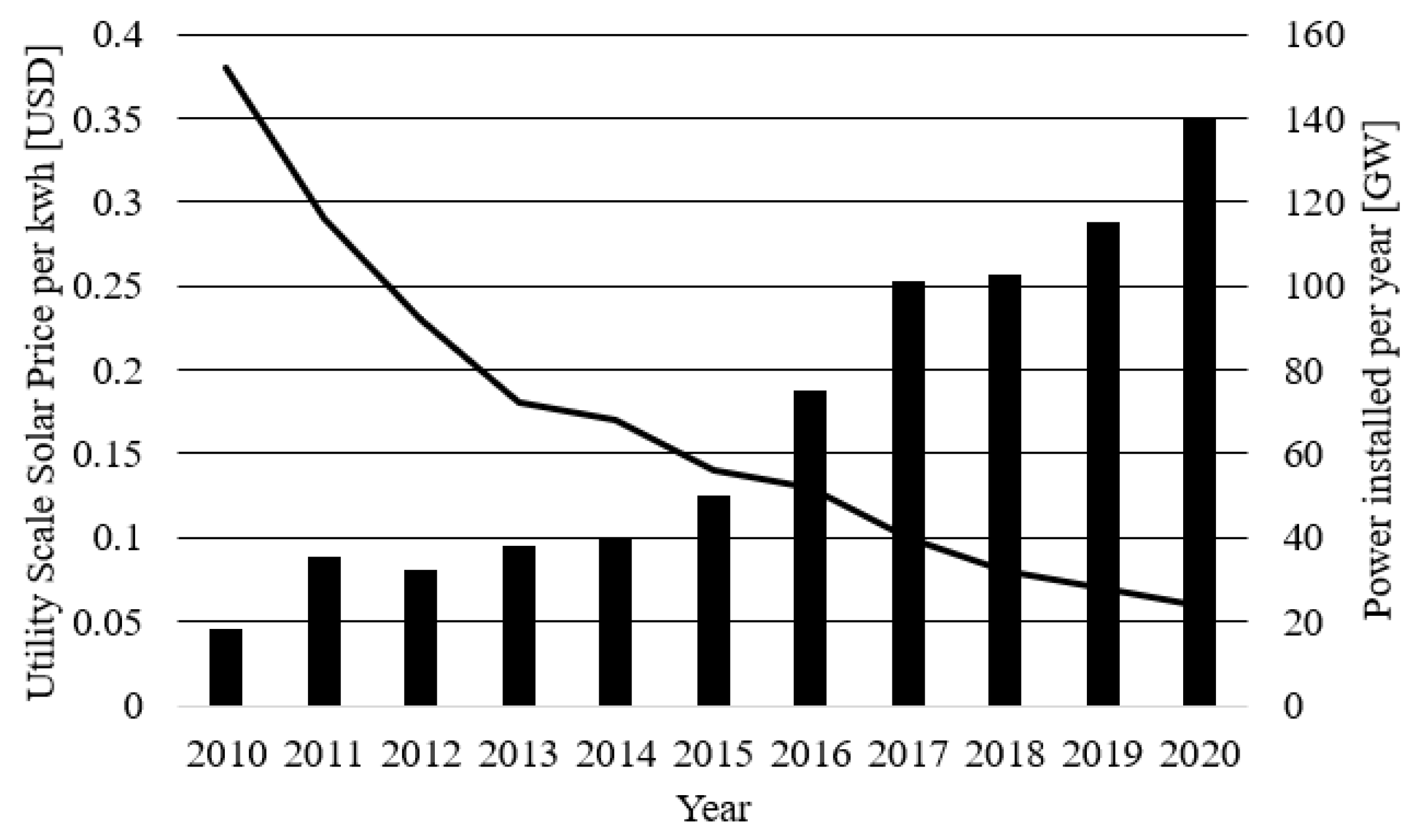
Globally, the PV power generation market in 2020 has installed 139.4, compared to 114.9 GW in 2019 [3], that is, an increase of 21.32%, which indicates the important growth of this type of power source (Figure 1). However, PV modules suffer degradation caused by aging, wear and tear, as well as their outdoor exposure [4], which causes their power to decrease, affecting the overall efficiency of the PV installation [5]. Therefore, preventive maintenance is required to know the current status of each module [6], and predictive maintenance to achieve comprehensive management [7]. In this way, the I–V tracer is a device that allows the extraction of parameters from the PV module to know exactly its current state [8].

This study presents a review of the different types of I–V tracers that exist in the bibliography, including rheostats, capacitive loads, electronic loads, transistors, or by means of DC–DC converters. The physical behavior of each of the strategies presented has been explained. Possible challenges that the operator may find in their use and design are also analyzed, focusing specifically on the power dissipated by the electronic components of the equipment. The paper shows the electrical parameters to which the electronic elements of the equipment are exposed using LTSpice, facilitating the appropriate topology selection. Additionally, a comparison has been included between the different I–V tracers’ topologies, analyzing their advantages and disadvantages concerning different factors such as their flexibility, modularity, cost, precision, speed or rating, as well as the characteristics of the different DC–DC converters.

2. I–V and P–V Curves Analysis

I–V and P–V curves allow characterizing a PV cell or module, giving the electrical parameters that describe the operation of the device under test. I–V and P–V curve analysis is usually an invasive technique to detect the deterioration of PV modules that consists of applying a variable load on the module terminals to obtain their current and voltage response. In this way, the analysis of the module response curves gives us direct information on the electrical "state" of the module, allowing the researcher to obtain data on the expected performance of the module under different conditions of solar irradiation and module load. However, it is an analysis that must be supported by other deterioration detection techniques to be able to give a conclusive answer [9], because in normal operating conditions, PV modules can develop several failure modes at the same time, which implies that the response of the characteristic curves is an addition of all faults of the module.

2.1. I–V and P–V Curves

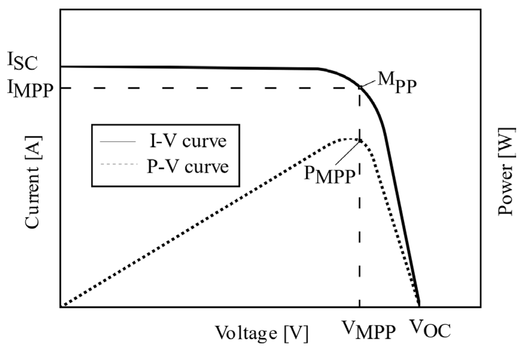
The best-known way to characterize a PV cell or module is to obtain its response curve, which gives voltage, current, and power information. These device responses are known as the I–V curve and the P–V curves, as shown in Figure 2. These characteristic curves provide important information about the state of the PV cell or module under analysis and are directly dependent on the temperature and radiation received by the module or cell.

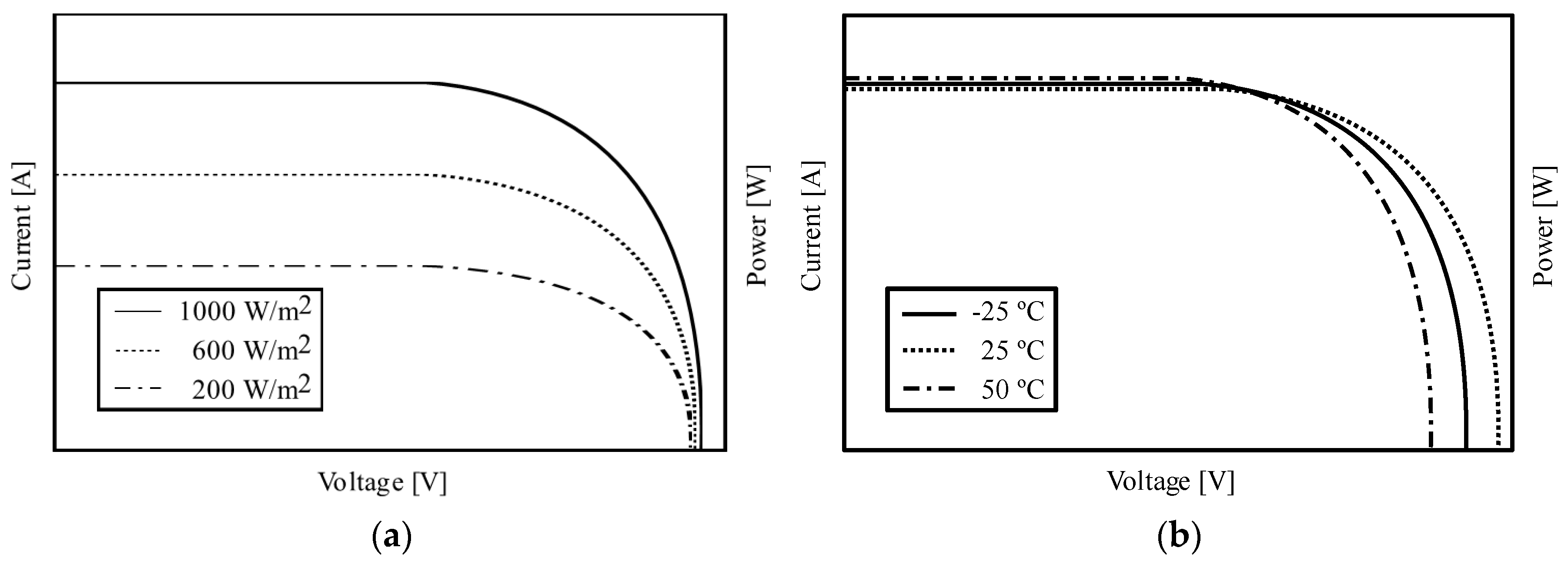
An I–V curve indicates the response of the PV module to different load conditions, at a known temperature and radiation. The dependence of the P–V curve with radiation is stronger than the dependence with temperature, thus, Figure 3a shows the response of a PV cell to different levels of radiation, where it is observed that the short-circuit current (Isc) changes. Regarding its temperature dependence, Figure 3b shows the variation of the open circuit voltage (Voc) at different temperatures.

2.2. Deviations from the I–V Curve

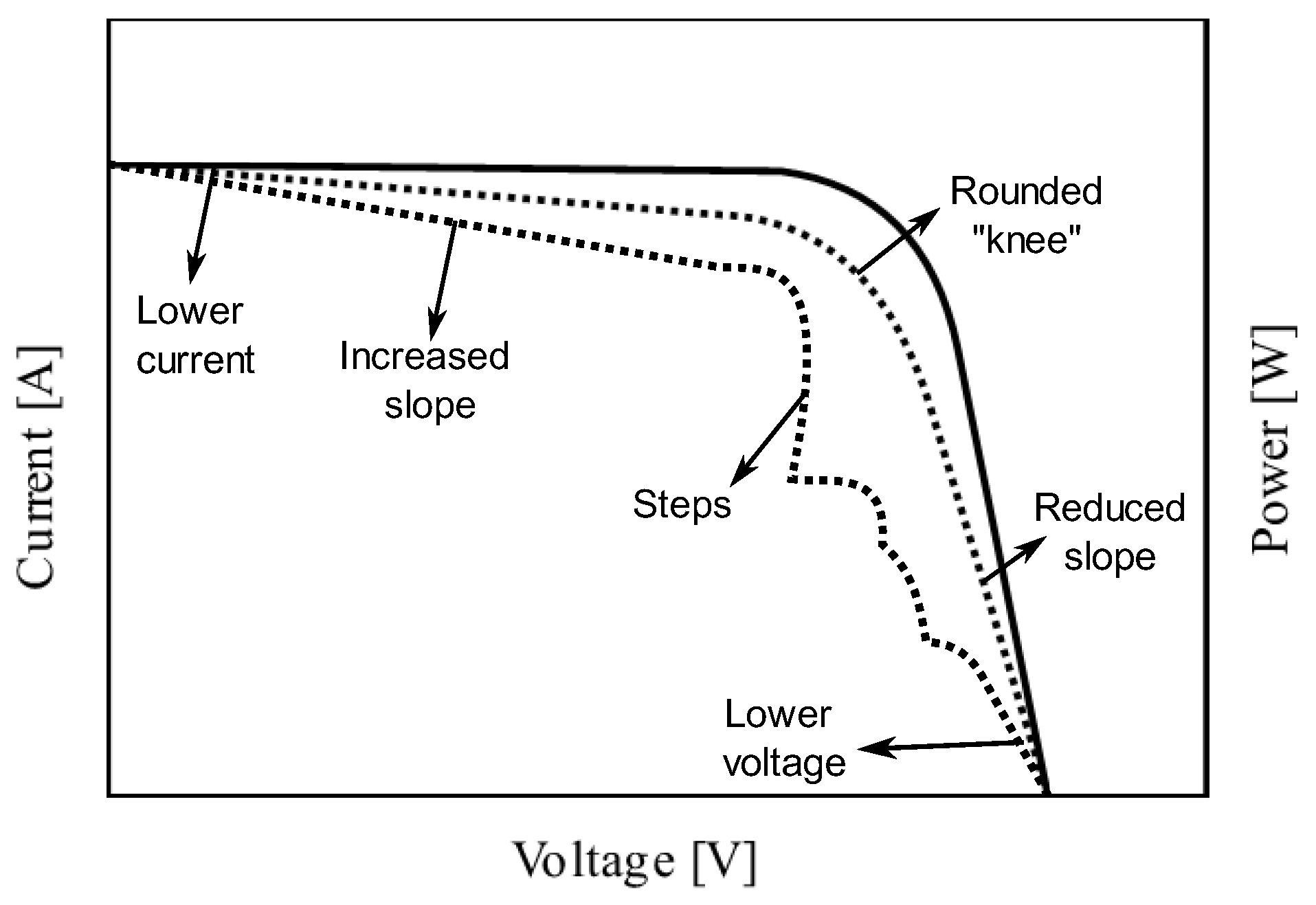
When a PV module shows deterioration, the I–V curve also presents deviations compared to a curve of a faultless module. Deviations in the I–V curves correspond to different causes of deterioration and represent a different type of failure in a PV generator. They can also be caused by errors at the time of the configuration of the curve sampling equipment, connection errors between the equipment and the module, high cloudiness or radiation interference when taking the measurement, etc., so when capturing the curve, these drawbacks should be avoided. Figure 4 shows the possible deviations that can be found in an I–V curve.

The deviations of the I–V curve listed in Figure 4 and established in [12] are the following:

• Steps or “ladder”. A deviation observed as steps or a “ladder” can be caused by partial shading, dust deposit, cracked cells, or a short circuit in the bypass diode.
• Low current. An I_SC below the nominal can be caused by the uniform deposit of dust or the normal degradation of the module.
• Low voltage. A V_OC lower than nominal can be caused by thermal module stress (hot spot or module temperature above STC), completely shaded cells, or bypass diode failure.
• Rounder “knee”. If the inflection point of the curve or “knee” is rounder than that observed in a nominal curve, it may be the cause of aging of the module that can be evidenced by the change in the values of the series and parallel resistances of the model of a diode.
• Slope reduction. The reduction of the slope on the upper part or “horizontal leg” of the I–V curve can be caused by a dust deposit located on the edge of a cell, due to a mismatch between the I_SC of the cells of a module (a reference to the quality of the cells), due to the presence of currents through the parallel branch of the diode model (which appear as short circuits of cracked cells), or due to hot spots.
• Increased slope. The increase in the slope in the right side or “vertical leg” of the I–V curve can be caused by the increase in the serial resistance of the module, or by excessive resistance of the connecting cables between modules.

2.3. Model of a PV Cell

Like any electrical generator, a PV module or cell can be modeled using its electrical characteristics, considering that this model must predict the electrical output of the cell under different types of operating conditions. Numerous models have been made in order to simulate the performance of solar cells [13]. The single-diode model is the most widely used. Three equivalent circuit models can be used to describe a single-diode model. The first of them is the ideal solar cell, also called 1M3P model (Single Mechanism, Three Parameters). For an ideal model, a solar cell can be simply modelled by a p-n junction in parallel with a current source that is associated to the photo carriers generated. The three parameters are the illumination current associated to the photoelectric effect, I_L, the reverse bias saturation current for the diode, I₀, and n, the diode ideality factor. More accuracy can be introduced to the model by adding a series resistance. The solar cell with series resistance, commonly known as 1M4P model (Single Mechanism, Four Parameters), takes into account the influence of contacts by means of a series resistance R_S. 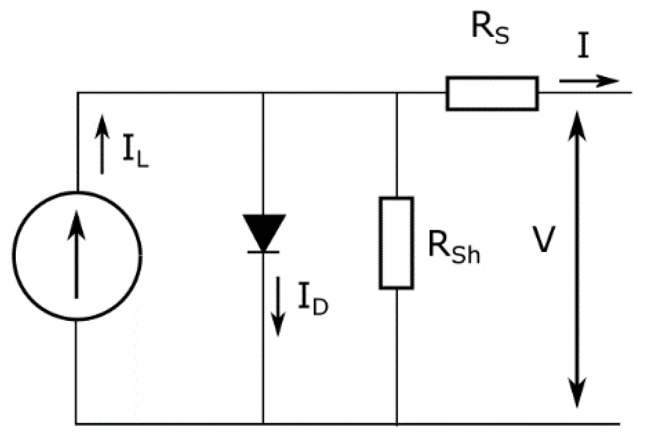The unknown parameters of this model are: I_L, I₀, n, and R_S. These models are not accurate enough, as they do not take into account some real factors in the solar cells. For that, it is necessary to introduce one more precise and realistic solar cell model. It is the solar cell with series and shunt resistances, 1M5P model (Single Mechanism, Five Parameters), shown in Figure 4. The R_Sh, parallel shunt resistor takes into account the leakage currents. The five parameters of this model are: I_L, I₀, n, R_S, and R_Sh [13]. The commonly used model is the one that represents the cell as a diode in parallel with a current source dependent on solar radiation [14] as shown in Figure 5, where the current delivered by the I_L PV generator is proportional to the solar radiation minus the currents flowing through the I_D diode and the R_SH parallel resistance.

The equivalent circuit shown can be used as a single cell, a multi-cell module, or an array of multiple modules. Considering temperature and constant radiation, the characteristic I–V of the 1M5P model is expressed by Equations (1) and (2):

$$I=I_L-I_D-I_{SH}=I_L-I_o\left[exp\left(\frac{V+I{R}_s}{a}\right)-1\right]-\frac{V+I{R}_s}{R_{SH}}$$

(1)

$$a=\frac{n{N}_{s}kT}{q}$$

(2)

where:

• I = current delivered by the PV generator;
• I_L = current induced by solar radiation;
• I_D = diode current;
• I_SH = current flowing through the resistance in parallel;
• I₀ = reverse saturation diode current;
• V = voltage at PV generator terminals;
• R_S = series resistance;
• R_SH = parallel resistance;
• a = modified ideality factor;
• k = Boltzmann constant (1.381 × 10⁻²³ [J/K]);
• T = cell temperature in degrees Kelvin;
• N_S = number of cells connected in series;
• q = electron charge (1.602 × 10⁻¹⁹ [C]);
• n = diode ideality factor (1 for ideal diodes and 2 for real ones).

The two-diode model introduces a second diode in parallel which takes into account the generation and recombination rates in the transition region of a p-n diode by introducing another diode in parallel, which may be significant under some thermal or illumination conditions in a high band gap semiconductor. At lower values of irradiance and low temperatures, the two-diode model gives more accurate curve characteristics than the single-diode model. Nevertheless, the number of equations and unknown parameters increases, making calculations more complex, as now there will be two unknown diode ideality factors. Therefore, the above-explained 1M5P model is widely used [13].

3. I–V Tracers’ Topologies

The drawing of I–V and P–V curves of a module is carried out using equipment called a tracer, which is electronic equipment capable of varying the load on the module or string terminals and taking measurements of corresponding voltages and currents. The equipment normally has a temperature sensor and a ration sensor, so that with these data, it is possible to perform the correction of the curve at STC. The correction is made following the standard IEC 60891: 2009 [15].

To obtain the I–V curve, different methods differ in their flexibility, fidelity, and cost. Obtaining the I–V curve is based on the variation of the current consumed at the terminals of the PV generator and its voltage response, so both electrical parameters must be measured either by automatic or manual methods [16].

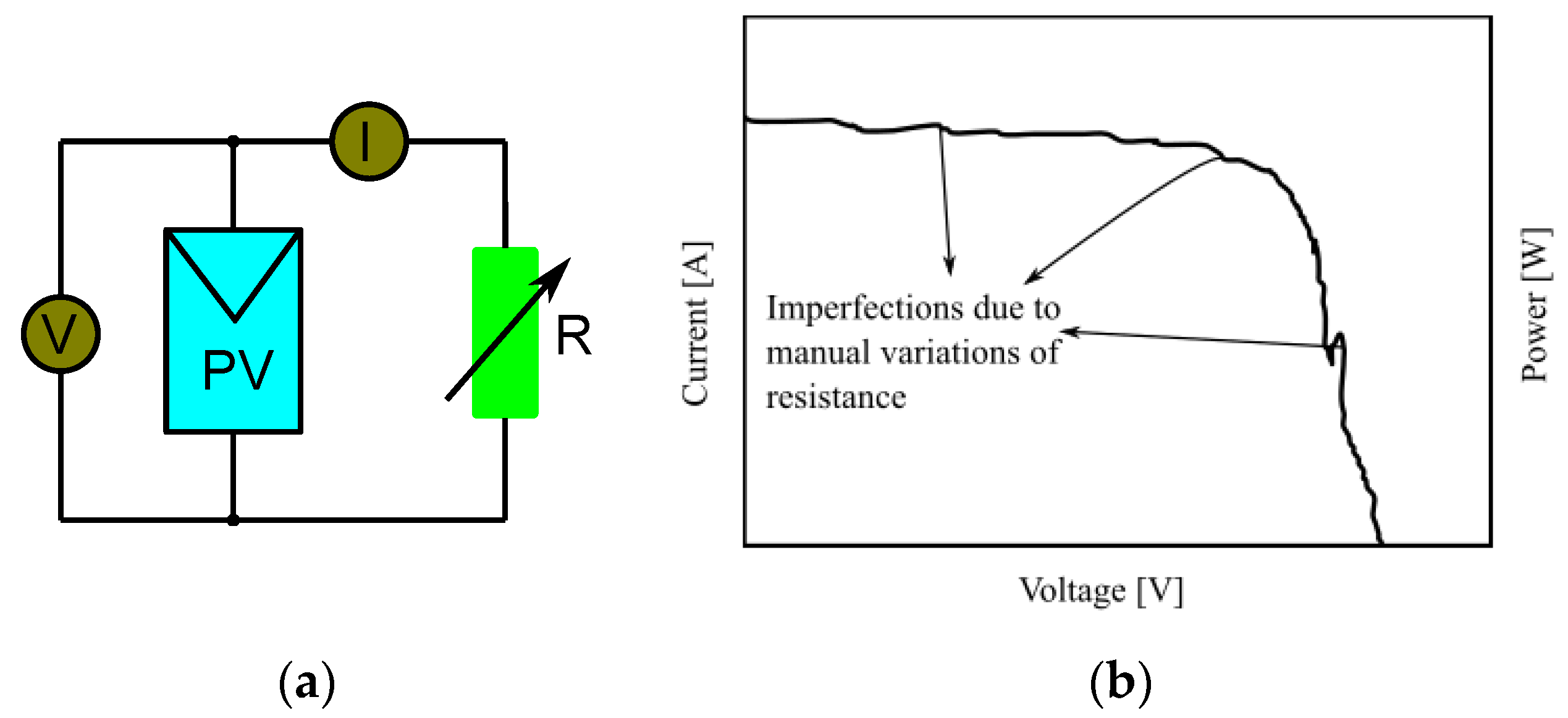
3.1. Variable Resistor Tracer or Rheostat

A variable resistor tracer is a device that can change the resistance in steps from zero to infinity (ideally) to capture points on the I–V curve (Figure 6). Normally, this method is applicable in low-power PV generators because high-power resistors are rare in the market.

This topology is used in [17,18,19,20], but it has limitations due to the quality of the curve obtained and the fact that the variation of resistance is normally done manually. In [9], the author states that the precision of the method is not high since it is susceptible to the fact that the solar radiation and the temperature vary while the test is carried out, and that the I–V curve does not have uniformity, and a high-power rheostat is not common in the market, making this method only applicable to low-power PV generators (<1 kW).

To improve the precision and fluidity of the curve in [17], a linear rheostat that is manually varied is used, in conjunction with a microcontroller with an external 12-bit analog–digital converter. In this way, the capture of current and voltage data is automated, increasing the number of points that can be obtained from the curve.

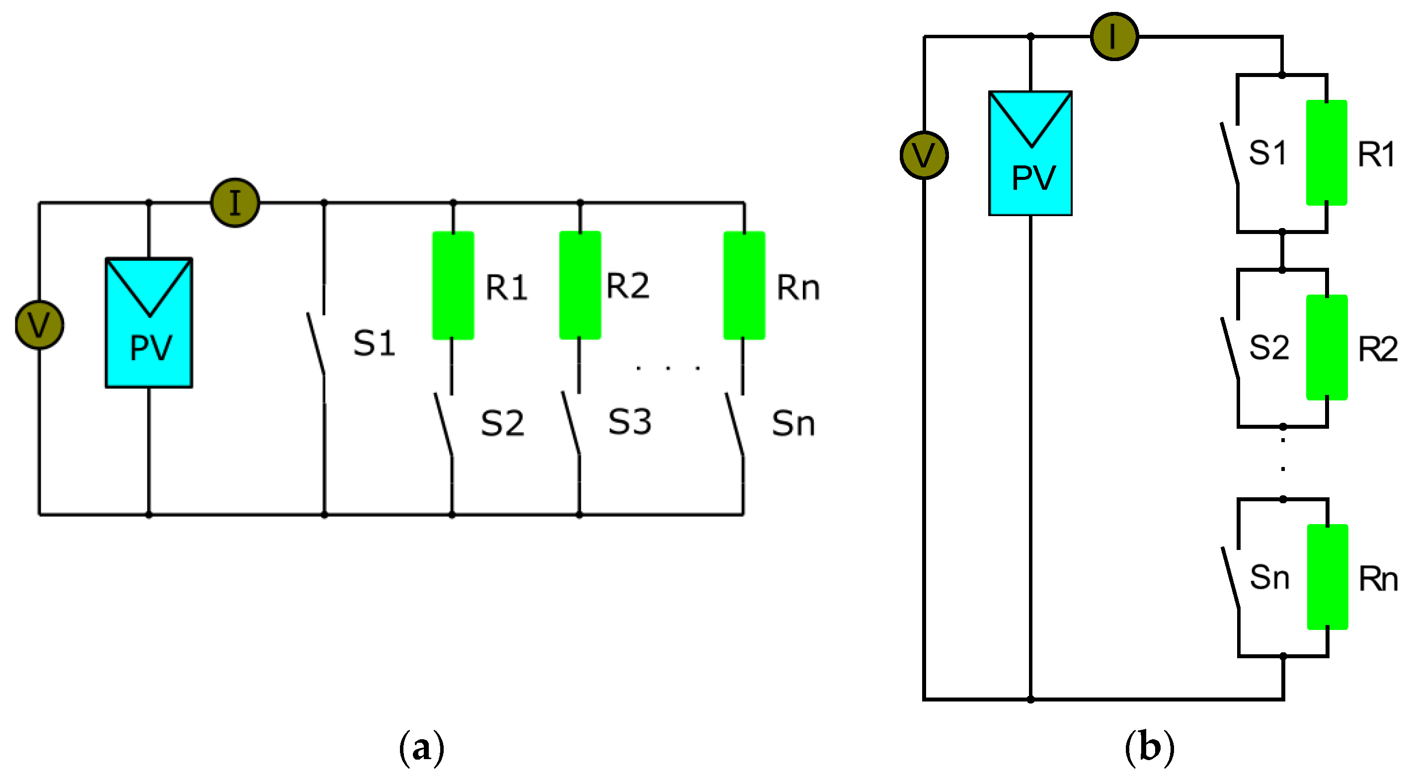
To improve the quality of the curve, in [21,22,23,24], diagrams of multiple resistors controlled by switches are presented to obtain the I–V curve (Figure 7), where its main limitation is the number of steps or points that can be obtained. In [21], a current and voltage sequencer is proposed, through the connection of resistors in parallel, automated by a computer, where the resistances must be selected appropriately to obtain a well-defined “knee”. In [22], a similar methodology is proposed, with the difference that the switches are MOSFETs, and the interface with the computer is an Arduino with a 12-bit external ADC. To increase the number of steps of this type of tracer, in [23], a binary scheme is proposed, where the resistors are in series and their activation depends on normally closed relays. Thus, in the case of a tracer with eight resistors, 255 different resistance values could be obtained for the elaboration of the I–V curve. In [24], LabView is used to capture the curve and carry out previous analyses.

The use of variable resistors placed as a load in a PV generator to obtain I–V curves is not recommended because with this method, the I_sc is not exactly reached, and the manual change of resistors takes considerable time, so the solar radiation and thermal conditions may change during measurement [16]. However, the cost advantages and ease of implementation and measurement automation of these types of tracers make them a viable alternative.

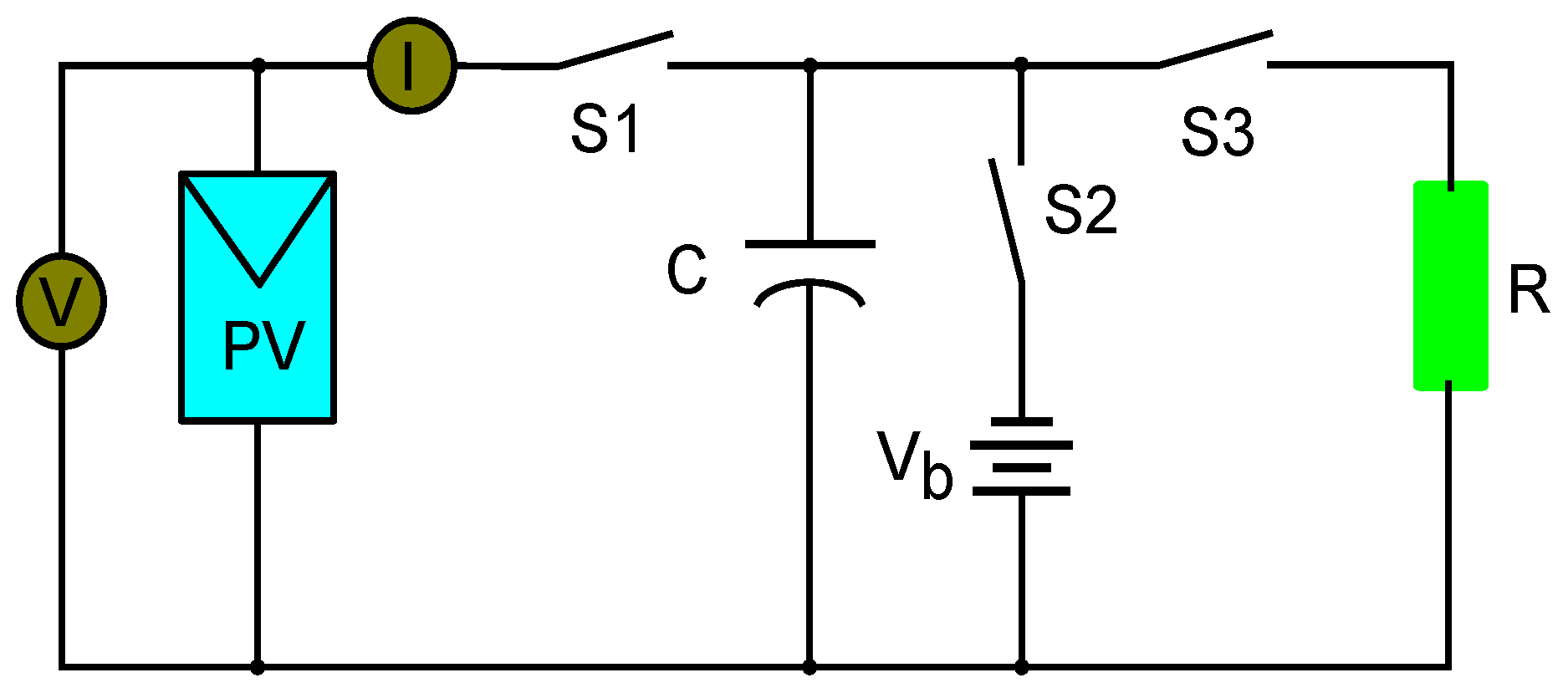
3.2. Capacitive Load Tracer

It is a capacitor-based method, where the capacitor is charged by the PV module forcing it to go from a short-circuit to an open-circuit condition. It is a widely used tracer. In [19], it is stated that the value of the capacitor suitable for this type of tracer depends directly on the short-circuit current and the open-circuit voltage, and is given by (3), based on the time of the establishment of the capacitor (t_S).

$$C=\frac{t_S}{2}\frac{I_{SC}}{V_{OC}}$$

(3)

In [25], the plotting time of the I–V curve is indicated with this method, and it is given by (4). The use of the tracer is proposed as part of an MPPT controller to identify possible shading conditions of the modules, which is also considered in [17].

$$T_{sweep}=1.261\left(\frac{V_{OC}·C}{I_{SC}}\right)$$

(4)

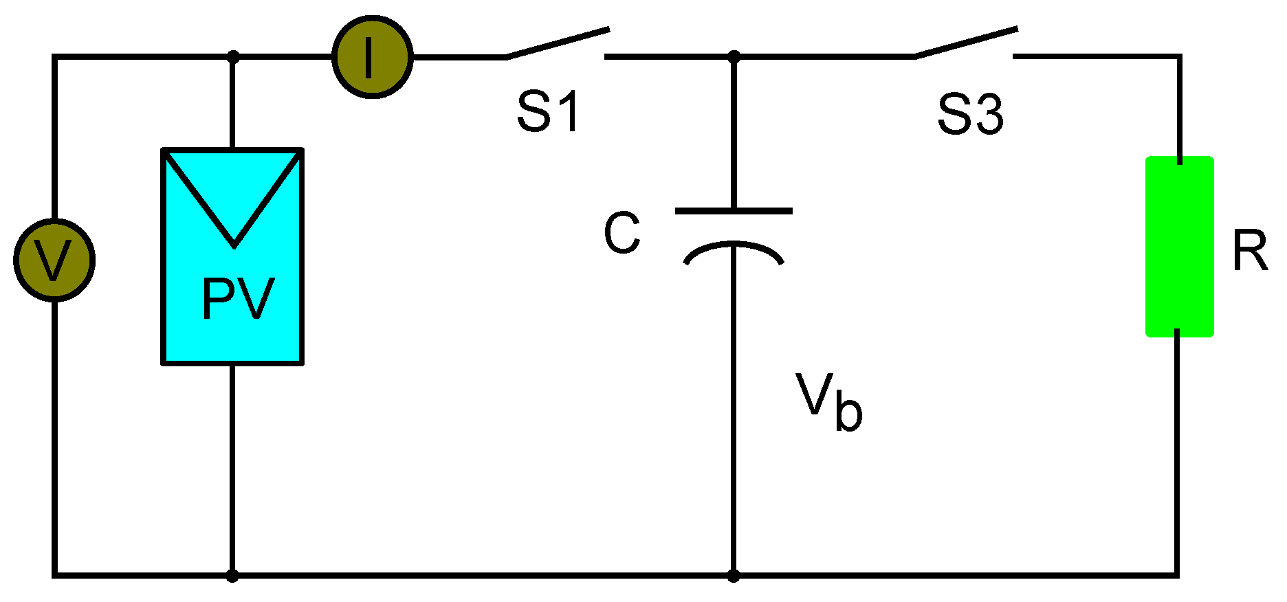
In Figure 8, the schematic of a capacitive tracer is shown, where before the measurement, the capacitor begins unloaded by S3 and R. When the measurement is to be started, S3 opens and S1 closes, so the PV generator has a very low load, reaching short-circuit condition. As the capacitor charges, the current decreases and the voltage increases, so when the charge ends, the current delivered by the module becomes zero, reaching the open-circuit condition. This scheme also allows starting the measurement with S2 closed, so that the capacitor would be charged to a negative voltage to reach I_sc exactly.

There are simpler topologies such as that shown in Figure 9, where only the capacitor and a discharge resistor are used.

For this type of tracer, the capacitors should be low ESR (equivalent series resistance) and low losses. The capacitance value depends on the required measurement time and has an impact on the measured voltage [26]. In this way, if short measurement times are required due to low capacitance values, the tracer design should consider voltage and current sensors that reach the necessary speed that may be in the order of milliseconds. Furthermore, depending on the current and voltage of the tracer, the use of IGBTs may be required for the proper triggering of the measurement stages, which increases implementation costs.

In [27], the effect of the arc produced by the connection of the capacitor is studied, which must be considered by the system converter. In [28], a genetic algorithm based on a bee colony is used to obtain the parameters of a PV cell after plotting its I–V curve with a capacitive tracer. In [29,30,31,32], the operation of this type of tracer, and different methods of connecting the capacitor, are discussed.

The low-cost advantage of this tracer has made it quite popular in the market, and it is even used in on-line tracers [33], that is, it is installed directly in the junction boxes of PV modules to measure their I–V curve regularly in a PV installation, constituting a semi-invasive measurement method as shown in Figure 10.

3.3. Electronic Load Tracer

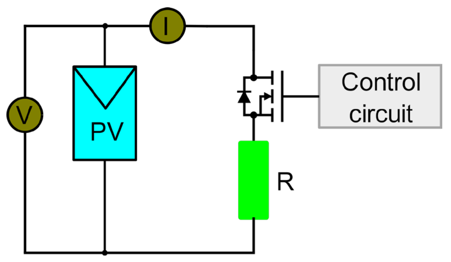
An electronic load tracer is a device that uses a transistor (MOSFET or IGBT) as a controlled load (Figure 11). It takes advantage of the resistance variation between the transistor terminals by modulating its gate voltage. Since the transistor could operate in any section of its characteristic curve, even in the ohmic region, it could be considered as an electronic variable resistance tracer.

These types of tracers use control circuits based on constant current loads and high-speed analog–digital converters. They have the advantage of being cheaper than the capacitive load for low voltages, with the limiting power that the transistors used in their design can handle, and they normally have noise in their measurement due to the transistor switching [34]. In [35], the use of a PWM control for the management of the MOSFET or an IGBT is proposed, and a structure for the galvanic isolation of the control circuit is exposed. In [36], this concept is extended, using a DAQ for the generation of a triangular signal as a control of the MOSFET. In [37], the characteristics of the MOSFET for its use in a tracer are studied.

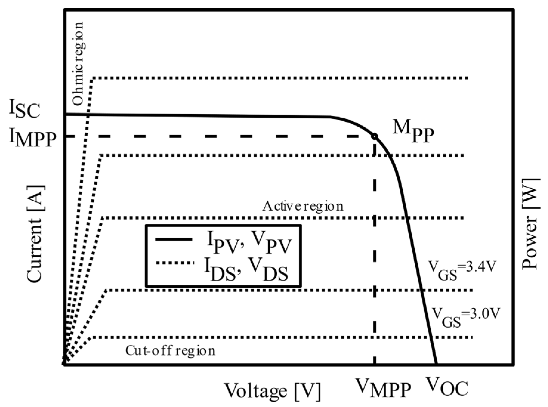
In [38], the application of conventional tracers is extended, adding a MQTT communication for the control of capacitive tracers. In [39], a low-cost tracer is designed, and information is gathered from studies to determine the characteristics of the MOSFET, specifically its characteristic curves, to properly select the transistor to be used based on the characteristics of the MOSFET (Figure 12) and the PV module. In [40,41,42], tracer designs with computer interfaces are carried out, both for the characterization of modules and for their use in solar plants.

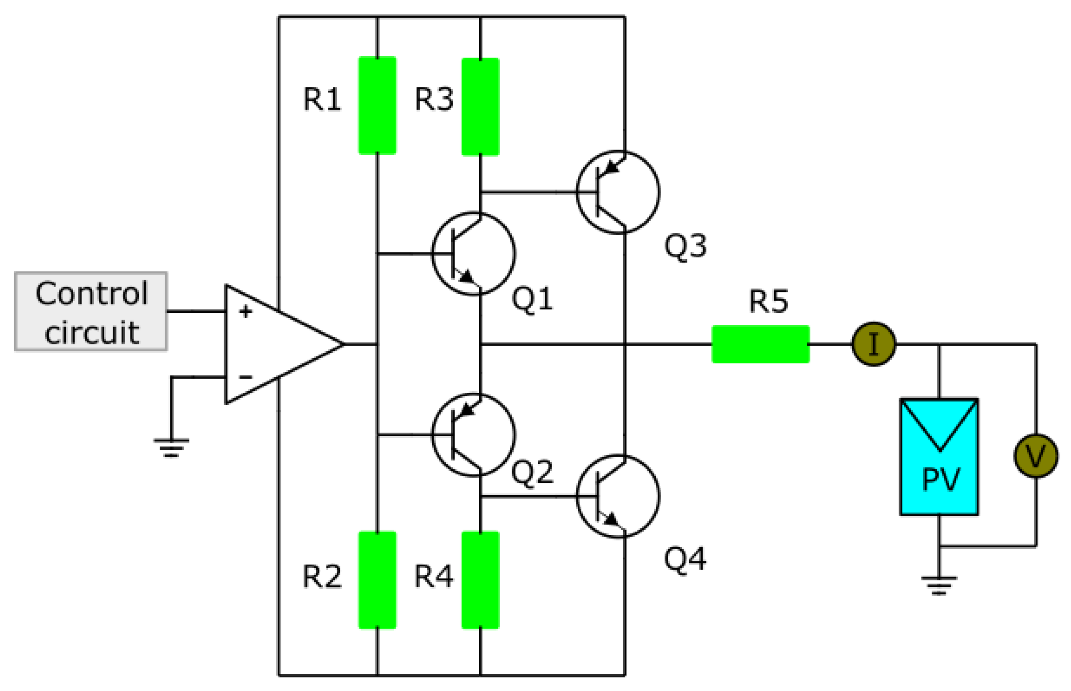
3.4. Bipolar Power Amplifier Tracer

It is a type of tracer that uses a configuration of bipolar transistors as class B power amplifiers (Figure 13) to allow the reversal of current and voltage for measurement of “dark” I–V curves (simulation of an I–V curve of a module in conditions without lighting). In [42], this type of tracer is used as a reference for the design of a solar simulator.

These tracers have the limitation of the use of BJT transistors in the linear area, so they are limited to low powers.

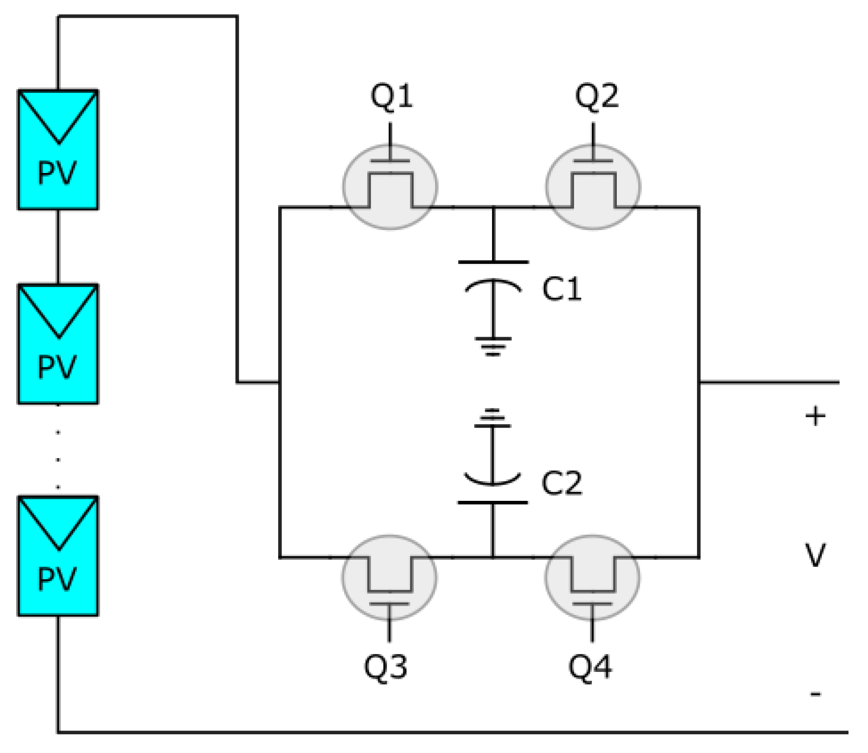
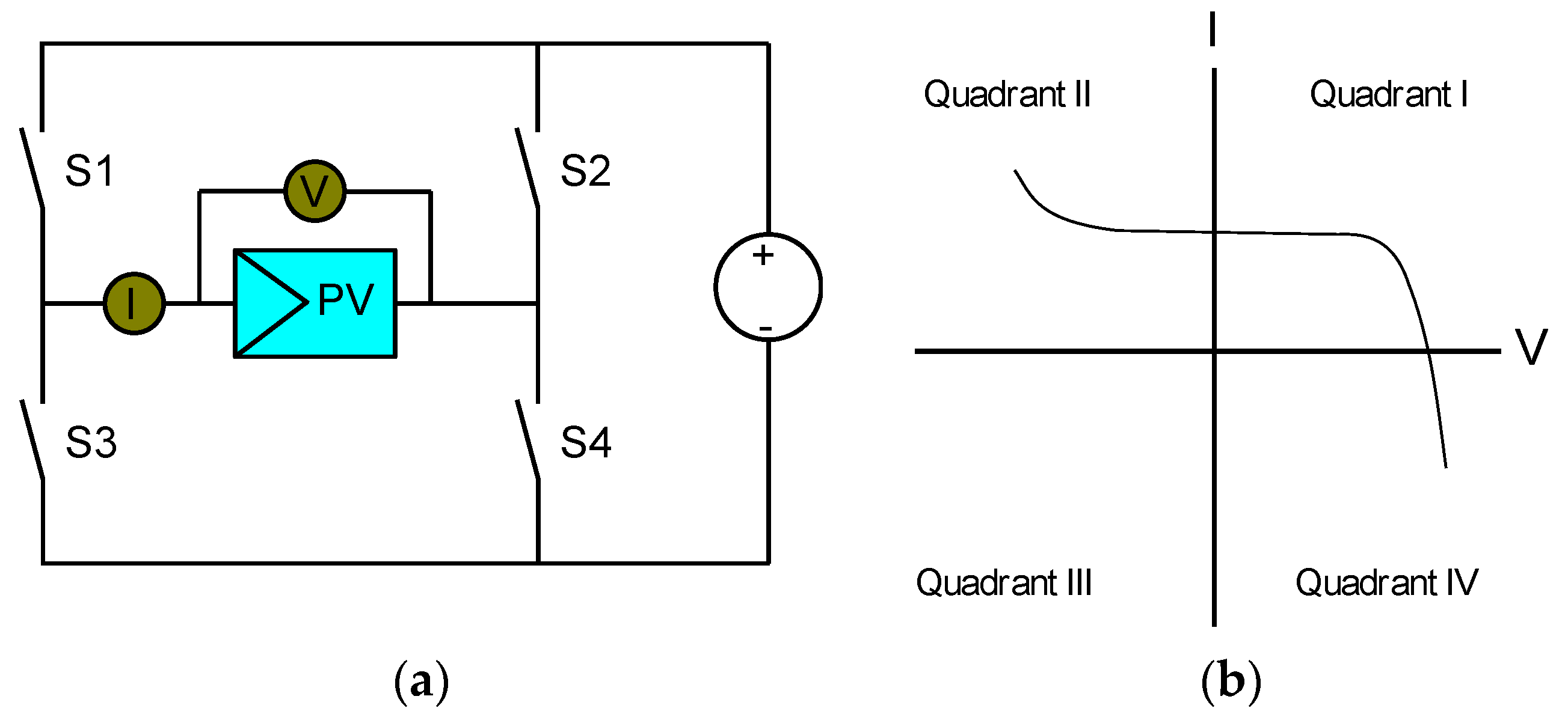
3.5. Four Quadrant Power Supply Tracer

It is a tracer based on a power source and transistors in H-bridge configuration that allows to deliver and consume energy from the PV generator to evaluate its performance in the four quadrants of an I–V curve (Figure 14).

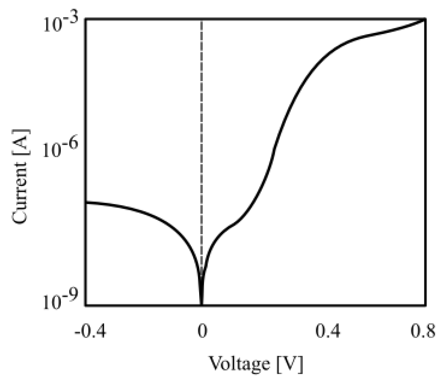
Investigation of the operation of four quadrants on a solar module allows the diagnosis of mismatches in partially shaded cells connected in series and is used for the generation of dark curves (dark I–V curve). The dark I–V curve is the curve of the module when it is non-illuminated, and specifically the current and voltage are measured when the module is powered by an external source. Figure 15 shows the dark IV curve of a solar module, from which the values of the series and parallel resistances and the ideality factors for the diode model can be obtained as well as the I–V curve correction methods to STC. In [43,44], methods for evaluating electrical module parameters with this type of curve are reviewed.

In [46], an experimental procedure is used to synchronize the measurement of two multimeters, to increase the precision of the measurement and reduce the uncertainty of this method. In [47], such a tracer is used to analyze module parameter extraction methods; in [48], it is used for high-efficiency cell analysis; and in [49], it is used to characterize modules and shading effects. Being a very precise method, in [50], it is used to verify the effect of series resistances introduced by the internal connection bars in a PV cell.

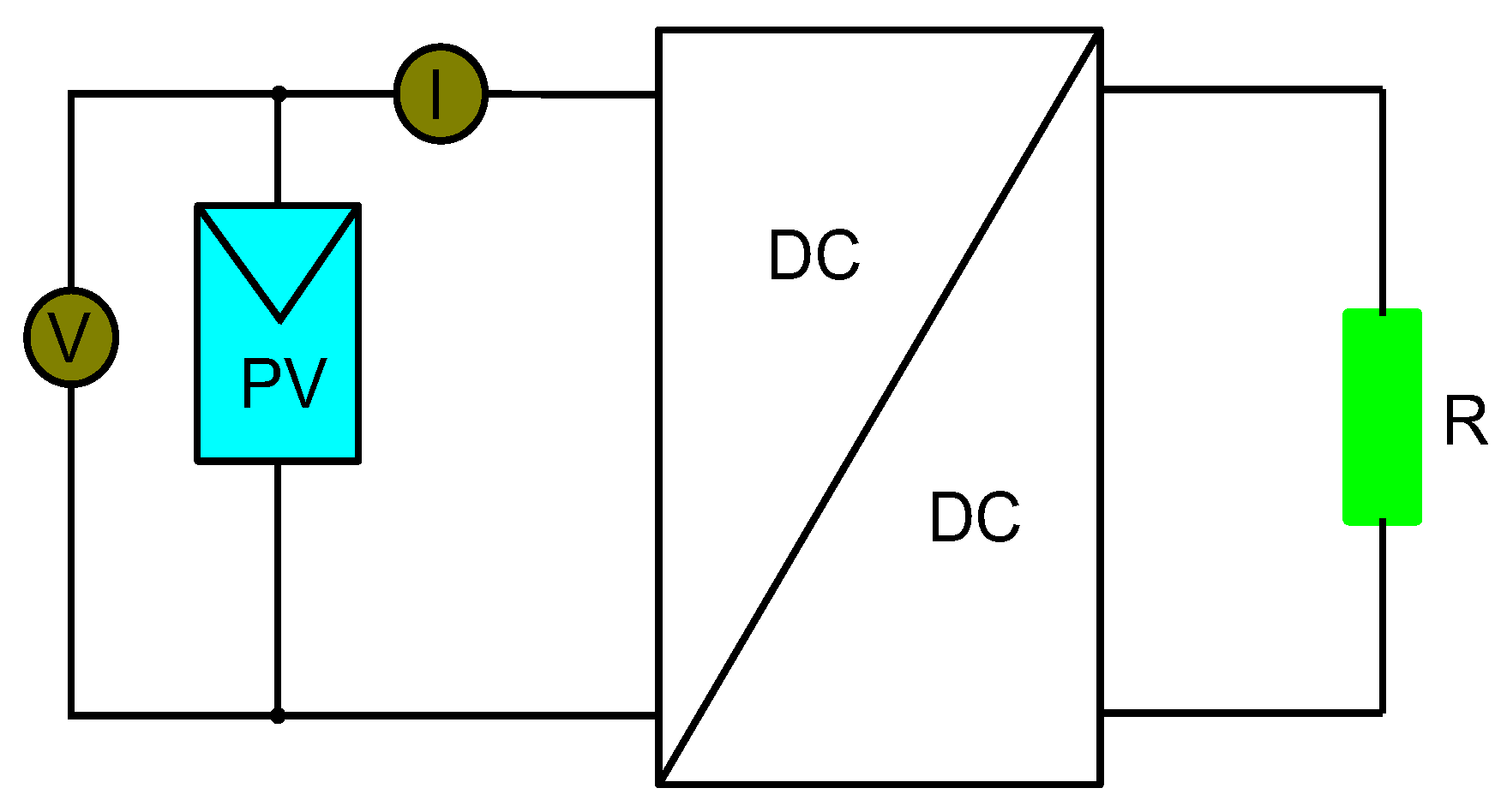
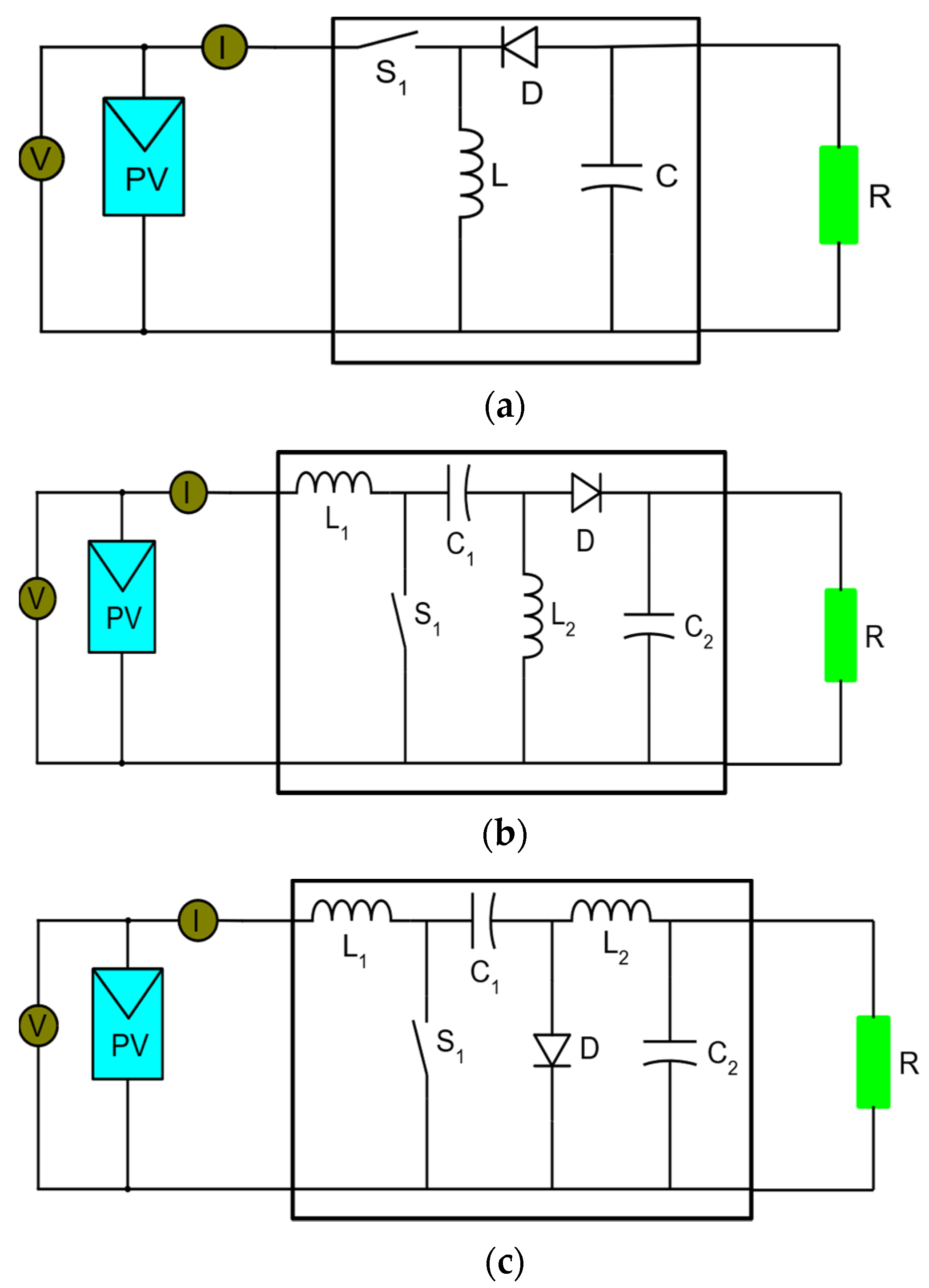
3.6. DC–DC Converter Tracer

It is a tracer based on the ability of DC–DC converters to emulate a resistor by varying its duty cycle (Figure 16). A DC–DC converter can plot the I–V curve of a PV generator in Buck-boost, Cuk, or Single-Ended Primary Inductor Converter (SEPIC) configuration [11].

In [51], the use of DC–DC converters as I–V curve tracers is proposed and in [52], this concept is extended by an automatic capture system with LabView. In [53,54], bidirectional DC–DC converters are used to obtain the I–V curves and to emulate the real-time behavior of a PV generator, and in [55], they are applied to MPPT (Maximum Power Point Tracking). In [56], the applications of DC–DC converters are analyzed as a variable electronic load. In [57], the control of DC–DC converters is studied using Switching-Frequency Modulation Scheme (SFMS) and its application in MPPTs.

As for the Buck-boost converters, they need to be of this topology since the Buck structures do not allow the drawing of points of the curve close to I_sc and the Boost structures cannot reach points close to V_oc [16]_.

Buck-boost converters have the disadvantage of introducing noise into the measurement due to the commutation of their internal elements (transistor and inductor), which is why leads from this circuit are used (Figure 17), known as Cuk converters and SEPIC [58]. They have a better frequency response and can be used as MPPTs as controllers for PV power generation. In [59], they use Cuk and SEPIC converters to decrease the ripple of the I–V curve caused by the commutation, and to reach the limits of I_sc and V_oc.

In [60], a SEPIC converter is used, with PWM control to generate the curve, and with Hall effect sensor for current measurement, and it is indicated that a four quadrant source can be used with this configuration. In [61], an adaptive control system is proposed, to ensure an optimal sampling rate.

In [62], two new methodologies are proposed, a voltage-controlled sweep to obtain more information on the “flat” part of I–V curve, and a current-controlled sweep for the rest of the curve: that is, a hybrid sweep. In [63], converters are used to obtain characteristics of PV generation systems by analyzing their frequency response, and Nyquist diagrams. In [64], the authors propose the use of SEPIC converters installed in line with strings for automatic I–V curve tracing within a PV installation.

The application of a Cuk converter and a control method for plotting curves and MPPT is discussed in [65]. In [66], the mathematical analysis of the Cuk converter and the details of its design are detailed. In [67], a digital control scheme of a Cuk converter is proposed for power factor correction, and its response to load variations.

4. Electrical Considerations in I–V Tracers

To select the appropriate topology when facing the design of an I–V tracer, it is of great importance to know the electrical parameters to which the electronic elements of the equipment are exposed. Therefore, this section will analyze the main types of topologies and the power, current, voltage, and temperature of the electronic components.

The simulation is carried out by controlling the switching element of the tracers, analyzing the electrical parameters of the elements of the different circuits. The results of powers, voltages, currents, and temperatures of the elements are compared to observe their maximum and minimum values in order to analyze electrical stress. To normalize the circuits, each type of tracer was designed to ensure equal power output, and the values were converted to per unit for percentage comparison. Real models of the circuit components were used; however, the limitations of the simulation such as variations in ambient temperature or leakage currents were not considered.

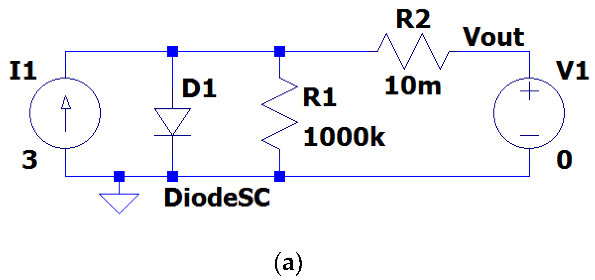
With this aim, the model of one diode of a PV cell (Figure 18a) is taken as a reference, in which an I_SC = 3 A and V_OC = 0.6239 V are imposed, with an M_pp = 1.476 W. Figure 18b shows the I–V and P-V curves of the cell. Because the voltage of a single cell is limited, a 5-cell circuit in series has been used, obtaining an I_SC = 3 A, V_OC = 3.1195 V, and M_pp = 7.38 W. Simulations were performed in LTSpice.

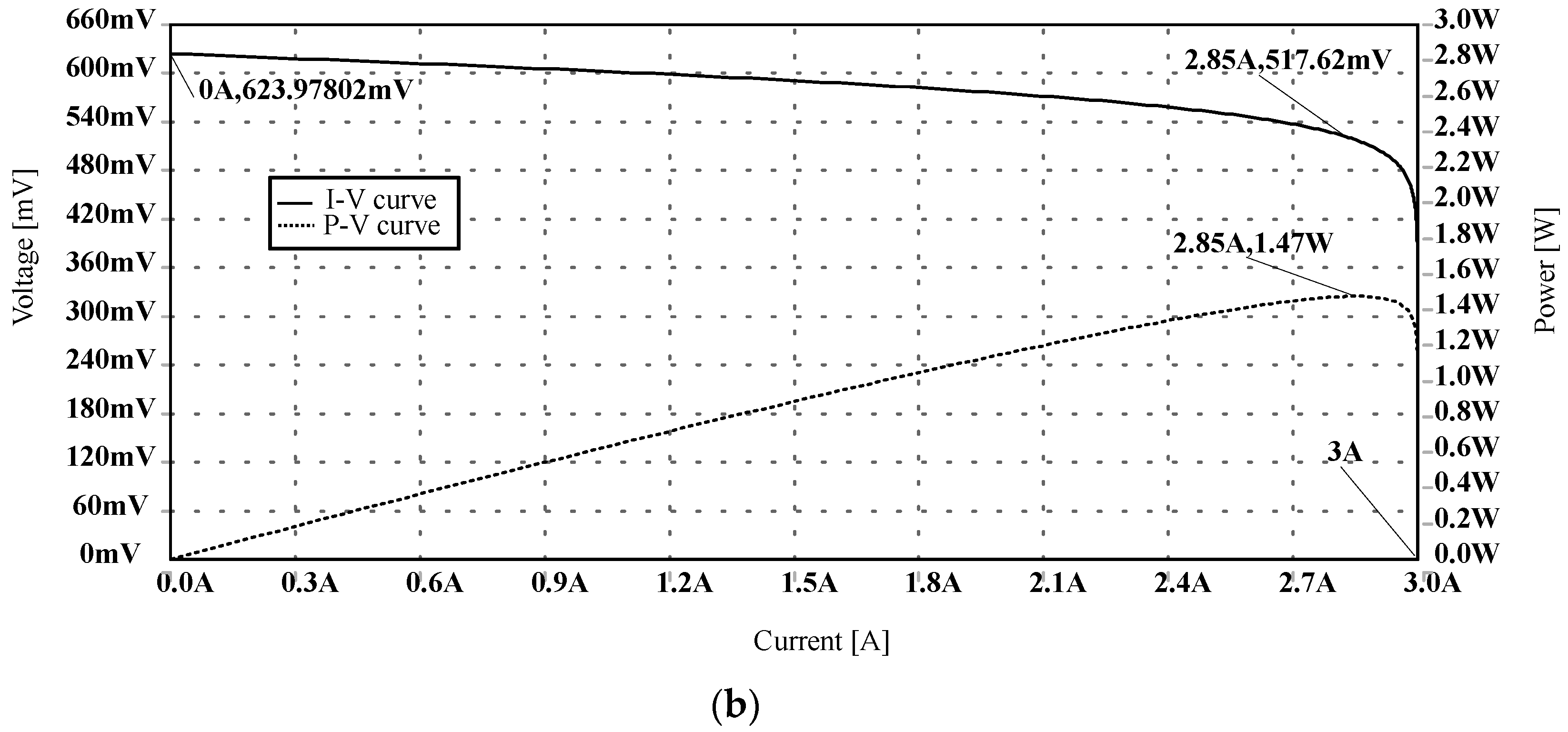
4.1. Variable Resistance, Electronic Load, and Capacitive Load Tracers

These three tracers are analyzed in this subsection for their similarity in their operating principle. Both the variable resistance and the switching element in an electronic load dissipate all the energy when drawing the I–V curve. Additionally, the capacitive load tracer, in the same way, has a single element (resistor) that dissipates the total power of the circuit.

For the variable resistance tracer (Figure 19a), it is observed that the power dissipated by the resistance is the total power of the cells, that is, their power dissipation is 1 p.u. compared to the module power. Additionally, all the current and the voltage of the module is dissipated on the resistor, meaning 1 p.u. for those parameters. Considering the temperature of 48.59 °C reached by a 10 W resistor, with a thermal resistance of 3.2 °C/W [68], and 25 °C as base ambient temperature, this parameter is 1.94 p.u.

Similarly, for the MOSFET-based electronic load tracer (Figure 19b), the power dissipated by the device is the total power of the module. However, in the electronic load, there is an additional resistor for the current measurement, and the internal resistance of the MOSFET, which causes the device to dissipate 7.3 W, that is, 0.98 p.u. for a short time. Regarding voltage and current at the electronic load, both parameters peak at 1 p.u., but the temperature rises up to 50.55 °C, which is 2.02 p.u.

In the case of the capacitive load tracer (Figure 19c), the resistor dissipates all the power, i.e., 1 p.u., during the charging time of the capacitor. Current and voltage are 1 p.u, and the temperature peaks at 2.02 p.u., the same that the temperature is shown as in the electronic load tracer, but in this case, the temperature remains high for a longer time.

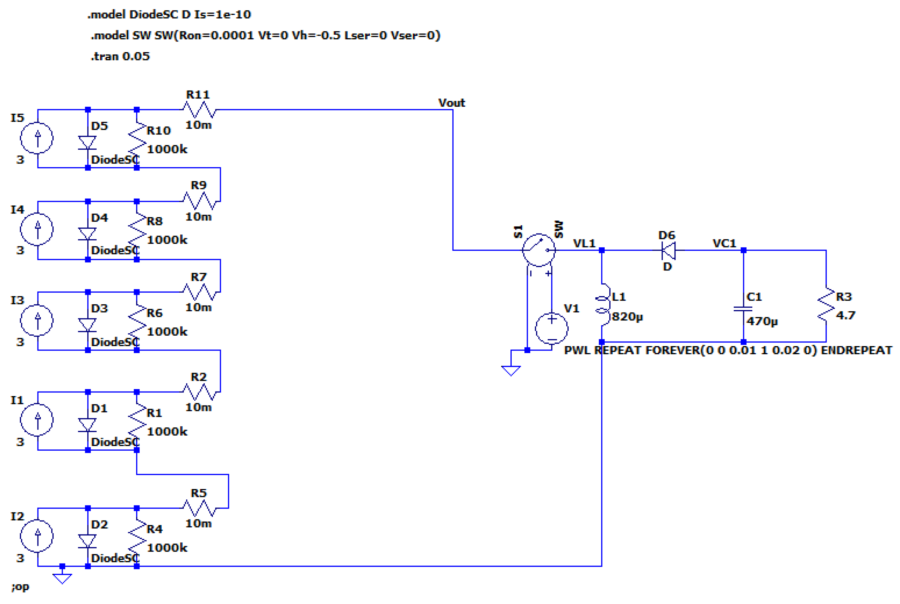
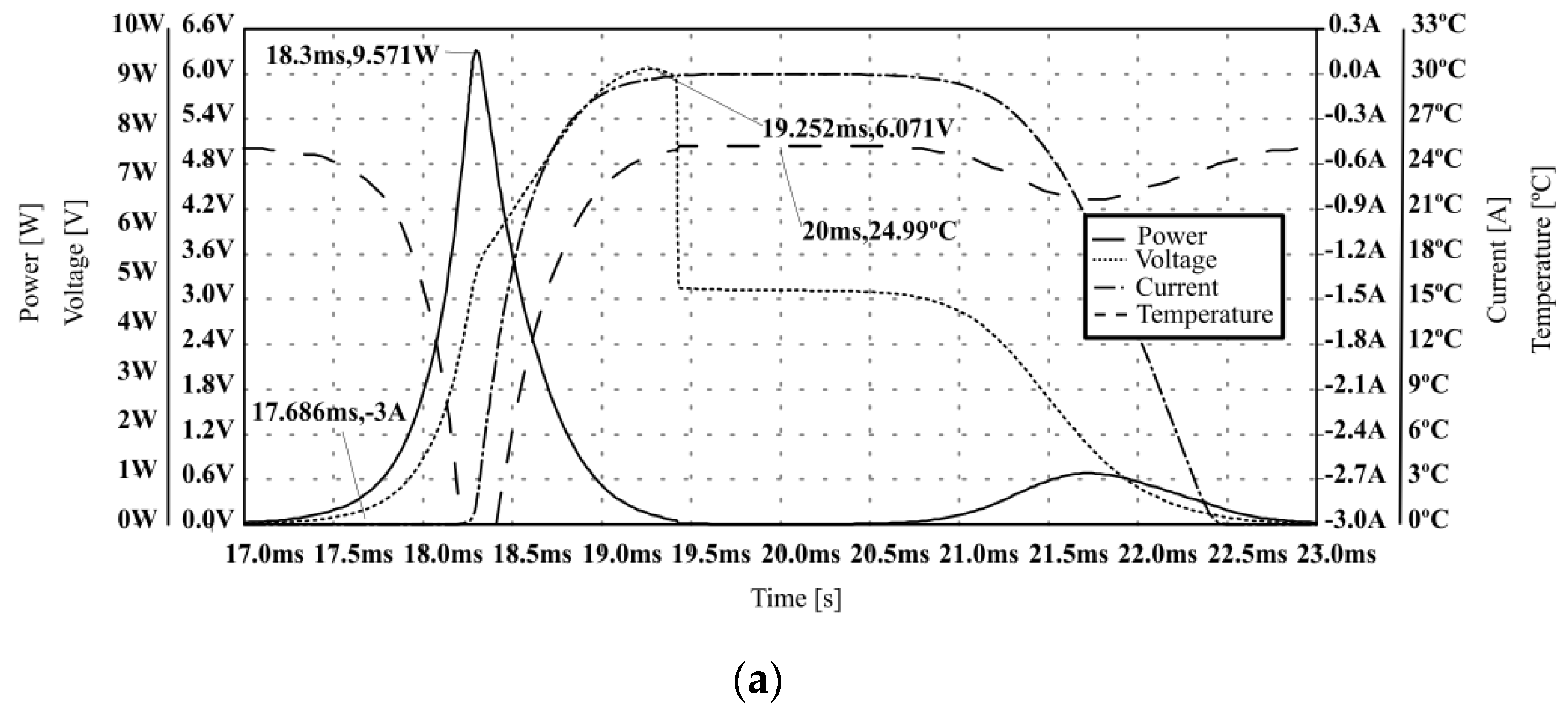
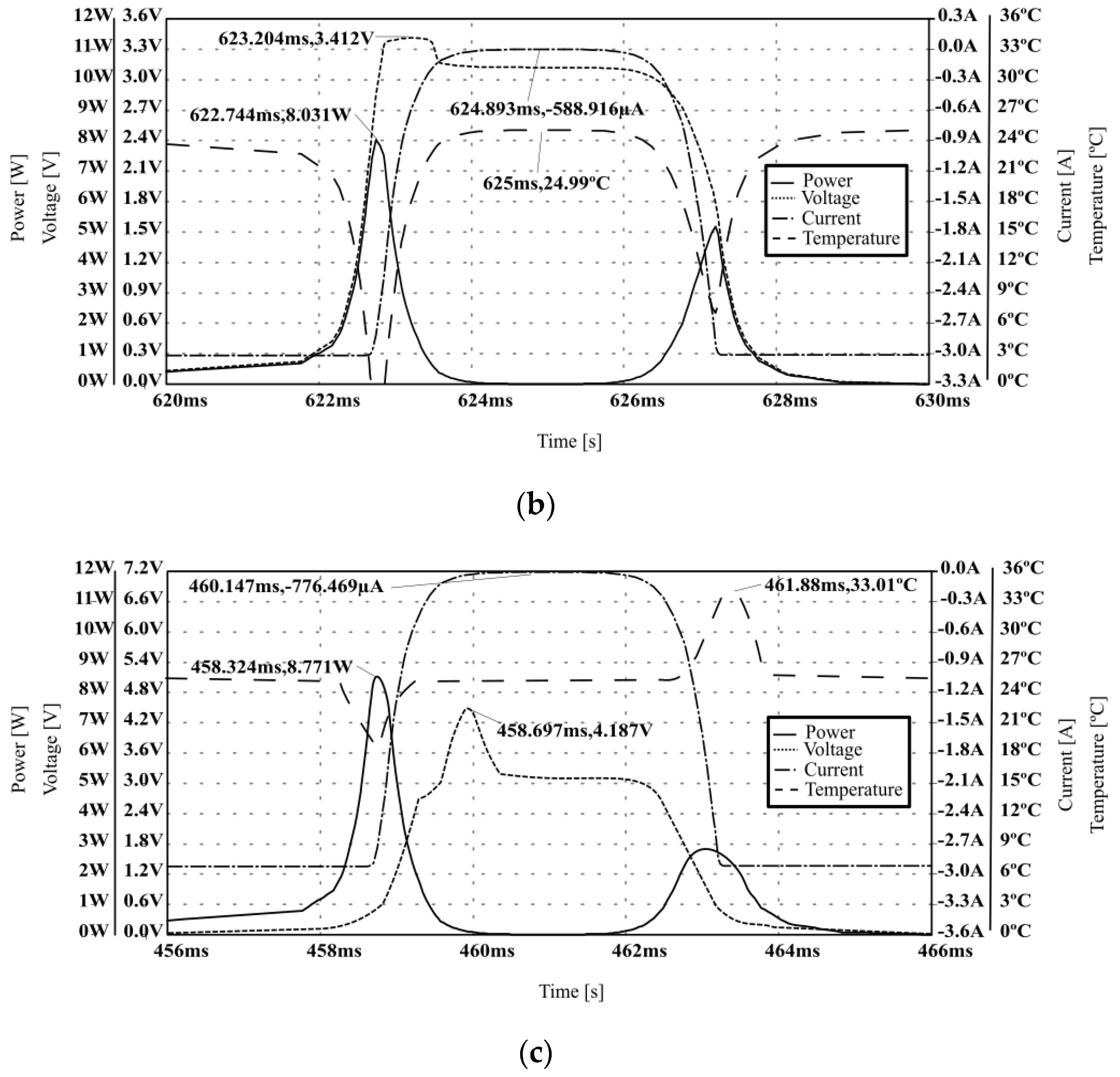
4.2. DC–DC Converter Tracers

Regarding the DC–DC converter-based tracers, Buck-boost, SEPIC, and Cuk converters are analyzed in this subsection. For all these types of converters, elements with values that ensure an output voltage of 1 p.u were used of the set of cells, to find only the difference in power in each one (Figure 20).

Thus, in the Buck-boost converter, it is obtained that the power in the resistance is 0.13 p.u., the diode 0.16 p.u., the inductor 0.92 p.u. and the switching element 1.29 p.u. The greater current, voltage, power, and temperature was found in the switching element (Figure 21a).

In the Cuk converter (Figure 21b), it is observed that the element that dissipates the most power is the switch with 0.98 p.u., and in the case of SEPIC (Figure 21c), likewise, the switch is the element that dissipates more power, in this case, 1.2 p.u., and inductor L1 with 0.36 p.u.

5. Discussion

The topologies of the I–V tracers analyzed in this study are the most widely used in the industry and they have evolved over the past 15 years. However, each has advantages and disadvantages that make them unique for specific applications and for studies that require obtaining certain electrical characteristics from PV generators (

Table 1. Comparison of the advantages and disadvantages of the analyzed I–V tracers’ topologies.

I–V Tracer Method	Flexibility	Modularity	Fidelity	Cost	Accuracy	Sweep Speed	Maximum Rating	Resolution
Resistive load	Medium	Medium	Medium	Low	Low	Low	Low	Low
Capacitive load	Low	Low	Medium	High	Medium	Medium	High	Medium
Electronic load	High	High	Medium	High	Medium	Medium	Low	Medium
Bipolar power amplifier	High	High	High	High	Medium	Medium	Low	Medium
4-Quadrant power supply	Low	Low	High	High	High	High	Low	High
DC–DC converter	High	High	High	Low	High	Medium	High	High

). To analyze the advantages and disadvantages of each topology, a study is carried out on the parameters that must be considered when choosing each topology.

One of the parameters that must be considered to analyze the application of the types of tracers studied is the flexibility for the expansion of the equipment or its design, because the variation of its configuration allows coupling to different conditions of the PV system. In this aspect, the DC–DC converters allow the greatest flexibility since its control can be modified with different trip signals, their duty cycle, and power direction, with which most of the I–V curve areas can be addressed. On the other hand, the capacitive load tracer is the one that allows the least flexibility, since only the sweep time of the curve can be modified according to the capacitance value used.

Another parameter is modularity, which allows the tracer to be expanded. In this aspect, the electronic loads, the bipolar amplifier, and the DC–DC converters stand out, because more channels can be added, and the constituent elements can be modified. In this regard, the capacitive load and the four-quadrant source present difficulties for its expansion.

Regarding the fidelity of the analyzed methods, the ones that deliver the most reliable data are the DC–DC converters, the bipolar amplifier, and the four-quadrant source, because they are the only ones that can reach real I_SC values of the analyzed device.

Cost is also a factor to consider in any tracer. Thus, the resistive load tracer is the least expensive, but is limited to low powers. On the other hand, both the electronic load and the DC–DC converter have high costs due to the switching elements and coils that are required for their operation.

The precision of the measurement is another parameter that must be considered, especially when working with cells where precise values of voltage and current are required. In this, the four-quadrant source and the DC–DC converters stand out, due to the control that they have over their operation and the algorithms existing in the bibliography. Electronic loads and capacitive loads are less accurate, but this can be improved with the use of robust ADCs.

Another important parameter is the sweep speed of the curve. In this, the four-quadrant source stands out for the ease of voltage control. In this aspect, capacitive loads can be very fast or very slow, depending on the charging time of the capacitor.

The maximum power is another important parameter since the applicability of the tracer depends on different PV installations. In this, capacitive loads and DC–DC converters stand out, which can be modified according to the installation requirement easily and economically compared to other methods.

Finally, it is important to have as many as possible measurement points along the curve to obtain a proper resolution. A greater number of points allows detailed studies to be carried out on the state of the PV module. In this regard, the source of four-quadrants and the DC–DC converter stands out.

Regarding DC–DC converters, it is necessary to analyze them separately, considering their topologies, for their correct use. For this, [11]

Table 2. Characteristics of different DC–DC converter topologies. Source [11], own elaboration.

Topology	Inductor	Input Capacitor	Output Capacitor	Power Mosfet	Efficiency
Buck-boost	High RMS current	High capacitance	High capacitance	High current rating	Very low
Cuk	Low RMS current	Low capacitance	Low capacitance	High current rating	High
SEPIC	Low RMS current	Low capacitance	High capacitance	Low current rating	High

presents a comparison of the converter topologies. It is observed that in the case of efficiency, the Cuk and SEPIC converters are better than the Buck-boost, which is inherent in their topology. In addition, it is observed that the SEPIC converter uses a lower current MOSFET than other topologies, which translates into a lower cost of implementation.

Table 3. Per unit electrical parameters of the elements in tracers.

Tracer	Element	V	I	P
Variable resistance	R	1	1	1
Electronic load	MOSFET	1	1	0.98
Capacitive load	C	1	1	-
Buck-boost	L1	0.81	1	0.92
	MOSFET	1.94	1	1.29
	D	1	0.59	0.16
	C	0.68	0.53	-
Cuk	L1	0.2	1	0.17
	MOSFET	1.09	1	0.98
	D	0.26	0.24	0.06
	L2	0.89	0.01	0.01
	C2	0.63	0.01	-
SEPIC	L1	0.38	0.365	0.36
	C1	0.23	0.68	-
	MOSFET	1.33	1	1.21
	D	0.26	0.18	0.01
	L2	1.11	0	0.06
	C2	0.85	0.04	-

shows the results regarding the analysis carried out of the electrical parameters in the I–V tracers. It is observed that in the case of the Buck-boost and SEPIC, the power of the switching element is greater than in the Cuk. Furthermore, it is observed that in the Buck-boost, the L1 inductance dissipates the highest power, which indicates that this element must be dimensioned considering this particularly.

6. Conclusions

A study is presented on the existing topologies of I–V tracers, analyzing parameters such as their flexibility, modularity, reliability, cost, precision, scanning speed, and resolution, as well as their advantages and disadvantages. The physical behavior of each of the strategies presented has been explained. Additionally, an analysis is performed on the power that each element dissipates in different topologies, to have a reference for the selection of the elements within the circuit of a tracer. Possible challenges that the operator may find in its use and design are also analyzed, focusing specifically on the power dissipated by the electronic components of the equipment.

It is observed that the tracers based on a capacitive load are widely used in the industry, due to their low cost and high sweep speed, so several commercial tracers which use this topology can be found. However, the use of tracers based on DC–DC converters is a trend due to their modularity, their precision, and the existence of these converters in MPPT systems integrated in inverters, which is a technical advantage that can be exploited in the future.

In the analysis of the dissipated power, it was observed that the variable resistance, electronic load, and capacitive load tracers dissipate all the power of the module under analysis, so this fact should be considered when it is necessary to carry out the complete PV module string tracing. Regarding the DC–DC converter-based tracers, it was observed that the switching element dissipates the greatest amount of power in all the topologies studied. As for the Buck-boost converter, the second element to consider is the inductor, which dissipates a 0.92 p.u. module power. The dissipated power has a direct impact on the tracer design, since it has a relationship with the equipment’s cooling system and it limits the element’s lifetime.

Authors consider that the trend of actual measurement systems is to advance in three ways. On the one hand, it is necessary to have low-cost measurement systems. On the other hand, online measurements are very interesting, since they will allow measurement without disconnection of PV modules from the string. In addition, the measurements must be accompanied by low-cost communication systems, which allow data to be transmitted and synchronized in PV systems.

References

- REN21 Secretariat. Renewables 2020 Global Status Report; REN21: Paris, France, 2020. [Google Scholar]
- Sarikh, S.; Raoufi, M.; Bennouna, A.; Benlarabi, A.; Ikken, B. Implementation of a plug and play I-V curve tracer dedicated to characterization and diagnosis of PV modules under real operating conditions. Energy Convers. Manag. 2020, 209. [Google Scholar] [CrossRef]
- International Energy Agency. Snapshot of Global PV Markets 2021. 2021. Available online: https://iea-pvps.org/snapshot-reports/snapshot-2021/ (accessed on 1 January 2021).
- Dhimish, M.; Alrashidi, A. Photovoltaic degradation rate affected by different weather conditions: A case study based on pv systems in the uk and australia. Electronics 2020, 9, 650. [Google Scholar] [CrossRef] [Green Version]
- Gallardo-Saavedra, S.; Hernández-Callejo, L.; Alonso-García, M.; Santos, J.D.; Morales-Aragonés, J.I.; Alonso-Gómez, V.; Moretón-Fernández, Á.; González-Rebollo, M.Á.; Martínez-Sacristán, O. Nondestructive characterization of solar PV cells defects by means of electroluminescence, infrared thermography, I-V curves and visual tests: Experimental study and comparison. Energy 2020, 205, 1–13. [Google Scholar] [CrossRef]
- Baklouti, A.; Mifdal, L.; Dellagi, S.; Chelbi, A. An optimal preventive maintenance policy for a solar photovoltaic system. Sustainability 2020, 12, 4266. [Google Scholar] [CrossRef]
- Bosman, L.B.; Leon-Salas, W.D.; Hutzel, W.; Soto, E.A. PV system predictive maintenance: Challenges, current approaches, and opportunities. Energies 2020, 16, 1398. [Google Scholar] [CrossRef] [Green Version]
- Oulcaid, M.; El Fadil, H.; Ammeh, L.; Yahya, A.; Giri, F. Parameter extraction of photovoltaic cell and module: Analysis and discussion of various combinations and test cases. Sustain. Energy Technol. Assess. 2020, 40, 100736. [Google Scholar] [CrossRef]
- Dávila-Sacoto, M.; Hernández-Callejo, L.; Alonso-Gómez, V.; Gallardo-Saavedra, S.; González-Morales, L. Low-cost infrared thermography in aid of photovoltaic panels degradation research. Fac. Ing. Univ. Antioq. 2020. [Google Scholar] [CrossRef]
- Hashim, E.T.; Abbood, A.A. Temperature effect on photovoltaic modules power drop. Al-Khawarizmi Eng. J. 2015, 11, 62–73. [Google Scholar]
- Zhu, Y.; Xiao, W. A comprehensive review of topologies for photovoltaic I–V curve tracer. Sol. Energy 2020, 196, 346–357. [Google Scholar] [CrossRef]
- International Electrotechnical Commission. IEC 62446. 2006. Available online: https://webstore.iec.ch/publication/28628 (accessed on 1 February 2021).
- Gallardo-Saavedra, S.; Karlsson, B. Simulation, validation and analysis of shading effects on a PV system. Sol. Energy 2018, 170, 828–839. [Google Scholar] [CrossRef]
- John, A.; Duffie, W.A.B. Wiley: Solar Engineering of Thermal Processes; John and Wailey and Sons: Hoboken, NJ, USA, 2013; ISBN 978-0470873663. [Google Scholar]
- International Electrotechnical Commission. IEC 60891. 2016, pp. 2–7. Available online: https://www.en.aenor.com/ (accessed on 5 March 2021).
- Duran, E.; Piliougine, M.; Sidrach-De-Cardona, M.; Galan, J.; Andujar, J.M. Different methods to obtain the I-V curve of PV modules: A review. Conf. Rec. IEEE Photovolt. Spec. Conf. 2008. [Google Scholar] [CrossRef]
- El Hammoumi, A.; Motahhir, S.; Chalh, A.; El Ghzizal, A.; Derouich, A. Low-cost virtual instrumentation of PV panel characteristics using Excel and Arduino in comparison with traditional instrumentation. Renew. Wind Water Sol. 2018, 5, 3. [Google Scholar] [CrossRef]
- Malik, A.Q.; Damit, S.J. Outdoor testing of single crystal silicon solar cells. Renew. Energy 2003, 28, 1433–1445. [Google Scholar] [CrossRef]
- Mahmoud, M.M. Transient analysis of a PV power generator charging a capacitor for measurement of the I-V characteristics. Renew. Energy 2006, 31, 2198–2206. [Google Scholar] [CrossRef]
- Rivai, A.; Rahim, N.A. A low-cost photovoltaic (PV) array monitoring system. In Proceedings of the CEAT 2013 IEEE Conference Clean Energy Technology, Langkawi, Malaysia, 18–20 November 2013; pp. 169–174. [Google Scholar] [CrossRef]
- Van Dyk, E.E.; Gxasheka, A.R.; Meyer, E.L. Monitoring current-voltage characteristics and energy output of silicon photovoltaic modules. Renew. Energy 2005, 30, 399–411. [Google Scholar] [CrossRef]
- Amiry, H.; Benhmida, M.; Bendaoud, R.; Hajjaj, C.; Bounouar, S.; Yadir, S.; Raïs, K.; Sidki, M. Design and implementation of a photovoltaic I-V curve tracer: Solar modules characterization under real operating conditions. Energy Convers. Manag. 2018, 169, 206–216. [Google Scholar] [CrossRef]
- Rahim, N.A.; Rivai, A. Binary-based tracer of photovoltaic array characteristics. IET Renew. Power Gener. 2014, 8, 621–628. [Google Scholar] [CrossRef]
- Gupta, A.K.; Chauhan, N.S.; Saxena, R. Real time I-V and P-V curve tracer using LabVIEW. In Proceedings of the 1st International Conference Innovation and Challenges in Cyber Security, ICICCS 2016, Greater Noida, India, 3–5 February 2016; pp. 265–269. [Google Scholar] [CrossRef]
- Bifaretti, S.; Iacovone, V.; Cina, L.; Buffone, E. Global MPPT method for partially shaded photovoltaic modules. In Proceedings of the Energy Conversion Congrress Exposition ECCE 2012, Raleigh, NC, USA, 15–20 September 2012; pp. 4768–4775. [Google Scholar] [CrossRef]
- Spertino, F.; Ahmad, J.; Ciocia, A.; Di Leo, P.; Murtaza, A.F.; Chiaberge, M. Capacitor charging method for I-V curve tracer and MPPT in photovoltaic systems. Sol. Energy 2015, 119, 461–473. [Google Scholar] [CrossRef] [Green Version]
- Xiong, Q.; Ji, S.; Liu, X.; Zhang, F.; Zhu, L.; Xiong, Q.; Feng, X.; Gattozzi, A.L.; Hebner, R.E. Detecting and localizing series arc fault in photovoltaic systems based on time and frequency characteristics of capacitor current. Sol. Energy 2018, 170, 788–799. [Google Scholar] [CrossRef]
- Chen, Z.; Lin, W.; Wu, L.; Long, C.; Lin, P.; Cheng, S. A capacitor based fast I-V characteristics tester for photovoltaic arrays. Energy Procedia 2018, 145, 381–387. [Google Scholar] [CrossRef]
- Spertino, F.; Sumaili, J.; Andrei, H.; Chicco, G. PV module parameter characterization from the transient charge of an external capacitor. IEEE J. Photovolt. 2013, 3, 1325–1333. [Google Scholar] [CrossRef]
- Aguilar, H.M.; Maldonado, R.F.; Navarro, L.B. Charging a capacitor with a photovoltaic module. Phys. Educ. 2017, 52. [Google Scholar] [CrossRef]
- Recart, F.; Mäckel, H.; Cuevas, A.; Sinton, R.A. Simple data acquisition of the current-voltage and illumination-voltage curves of solar cells. In Proceedings of the Conference Record 4th World Conference Photovoltaiv Energy Conversion, WCPEC-4, Waikoloa, Hawaii, 7–12 May 2006; pp. 1215–1218. [Google Scholar] [CrossRef]
- Muñoz, J.; Lorenzo, E. Capacitive load based on IGBTs for on-site characterization of PV arrays. Sol. Energy 2006, 80, 1489–1497. [Google Scholar] [CrossRef] [Green Version]
- Joglekar, A.V.; Hegde, B. Online I-V Tracer for per string monitoring and maintenance of PV panels. In Proceedings of the IECON 2018—44th Annual Conference of the IEEE Industrial Electronics Society, Washington, DC, USA, 21–23 October 2018; pp. 1890–1894. [Google Scholar] [CrossRef]
- Erkaya, Y.; Flory, I.; Marsillac, S.X. Development of a string level I-V curve tracer. In Proceedings of the 2014 IEEE 40th Photovoltaic Specialist Conference (PVSC), Denver, CO, USA, 8–13 June 2014; pp. 3104–3107. [Google Scholar] [CrossRef]
- Leite, V.; Batista, J.; Chenlo, F.; Afonso, J.L. Low-cost I-V tracer for photovoltaic modules and strings. In Proceedings of the 2014 International Symposium on Power Electronics, Electrical Drives, Automation and Motion, SPEEDAM, Ischia, Italy, 18–20 June 2014; pp. 971–976. [Google Scholar] [CrossRef] [Green Version]
- Sahbel, A.; Hassan, N.; Abdelhameed, M.M.; Zekry, A. Experimental performance characterization of photovoltaic modules using DAQ. Energy Procedia 2013, 36, 323–332. [Google Scholar] [CrossRef] [Green Version]
- Kuai, Y.; Yuvarajan, S. An electronic load for testing photovoltaic panels. J. Power Source 2006, 154, 308–313. [Google Scholar] [CrossRef]
- Papageorgas, P.; Piromalis, D.; Valavanis, T.; Kambasis, S.; Iliopoulou, T.; Vokas, G. A low-cost and fast PV I-V curve tracer based on an open source platform with M2M communication capabilities for preventive monitoring. Energy Procedia 2015, 74, 423–438. [Google Scholar] [CrossRef] [Green Version]
- Willoughby, A.A.; Osinowo, M.O. Development of an electronic load I-V curve tracer to investigate the impact of Harmattan aerosol loading on PV module pern2tkformance in southwest Nigeria. Sol. Energy 2018, 166, 171–180. [Google Scholar] [CrossRef]
- Henni, O.; Belarbi, M.; Haddouche, K.; Belarbi, E.H. Design and implementation of a low-cost characterization system for photovoltaic solar panels. Int. J. Renew. Energy Res. 2017, 7, 1586–1594. [Google Scholar]
- Leite, V.; Batista, J.; Chenlo, F.; Afonso, J.L. Low-cost instrument for tracing current-voltage characteristics of photovoltaic modules. Renew. Energy Power Qual. J. 2012, 1, 1012–1017. [Google Scholar] [CrossRef]
- Guvench, M.G.; Gurcan, C.; Durgin, K.; MacDonald, D. Solar simulator and I-V measurement system for large area solar cell testing. ASEE Annu. Conf. Proc. 2004, 12747–12753. [Google Scholar]
- Kaminski, A.; Marchand, J.J.; Fave, A.; Laugier, A. New method of parameters extraction from dark I-V curve. In Proceedings of the Conference Record of the Twenty Sixth IEEE Photovoltaic Specialists Conference—1997, Anaheim, CA, USA, 29 September–3 October 1997; pp. 203–206. [Google Scholar] [CrossRef]
- Guechi, A.; Chegaar, M.; Aillerie, M. Environmental effects on the performance of nanocrystalline silicon solar cells. Energy Procedia 2012, 18, 1611–1623. [Google Scholar] [CrossRef] [Green Version]
- Remes, Z.; Stuchlik, J. Pulse measurements of small area thin film μc-Si:H/ZnO:B photodiodes. IOP Conf. Ser. Mater. Sci. Eng. 2020, 726, 1–8. [Google Scholar] [CrossRef] [Green Version]
- Piliougine, M.; Carretero, J.; Mora-López, L.; Sidrach-de-Cardona, M. Experimental system for current-voltage curve measurement of photovoltaic modules under outdoor conditions. Prog. Photovolt. Res. Appl. 2011, 19, 591–602. [Google Scholar] [CrossRef]
- De Blas, M.A.; Torres, J.L.; Prieto, E.; García, A. Selecting a suitable model for characterizing photovoltaic devices. Renew. Energy 2002, 25, 371–380. [Google Scholar] [CrossRef]
- Fernández-Reche, J.; Cañadas, I.; Sánchez, M.; Ballestrín, J.; Yebra, L.; Monterreal, R.; Rodríguez, J.; García, G.; Alonso, M.; Chenlo, F. PSA Solar furnace: A facility for testing PV cells under concentrated solar radiation. Sol. Energy Mater. Sol. Cells 2006, 90, 2480–2488. [Google Scholar] [CrossRef]
- Hecktheuer, L.A.; Krenzinger, A.; Prieb, C.W.M. Methodology for photovoltaic modules characterization and shading effects analysis. J. Braz. Soc. Mech. Sci. 2002, 24. [Google Scholar] [CrossRef]
- Granek, F.; Zdanowicz, T. Advanced system for calibration and characterization of solar cells. Opto-Electron. Rev. 2004, 12, 57–67. [Google Scholar]
- Enrique, J.M.; Durán, E.; Sidrach-De-Cardona, M.; Andújar, J.M.; Bohórquez, M.A.; Carretero, J. A new approach to obtain I-V and P-V curves of photovoltaic modules by using DC-DC converters. In Proceedings of the Conference Record of the Thirty-First IEEE Photovoltaic Specialists Conference, 2005, Lake Buena Vista, FL, USA, 3–7 January 2005; pp. 1769–1772. [Google Scholar] [CrossRef]
- Bohórquezb, M.A.; Enrique, J.M.; Durán, E.; Sidrach-de-Cardona, M.; Carretero, J.; Andújar, J.M. Analysis and failures monitoring in pv panels by means of i-v and p-v curves using dc-dc converters. In Proceedings of the WREC 2005 (World Renewable Energy Congress), Aberdeen, UK, 22–27 May 2005; pp. 477–483. [Google Scholar]
- Sanchis, P.; Echeverría, I.; Ursúa, A.; Alonso, O.; Gubía, E.; Marroyo, L. Electronic converter for the analysis of photovoltaic arrays and inverters. PESC Rec. IEEE Ann. Power Electron. Spec. Conf. 2003, 4, 1748–1753. [Google Scholar] [CrossRef]
- Sanchis, P.; López, J.; Ursúa, A.; Marroyo, L. Electronic controlled device for the analysis and design of photovoltaic systems. IEEE Power Electron. Lett. 2005, 3, 57–62. [Google Scholar] [CrossRef]
- Marroyo, L.; Sanchis, P.; López, J.; Ursúa, A.; González, R.; Gubía, E. Equipment for the analysis of the maximum energy of real photovoltaic systems. IEEE Int. Symp. Ind. Electron. 2005, 3, 1031–1036. [Google Scholar] [CrossRef]
- Kazerani, M. A high-performance controllable DC load. IEEE Int. Symp. Ind. Electron. 2007, 1015–1020. [Google Scholar] [CrossRef]
- Tse, K.K.; Ho, B.M.T.; Chung, H.S.H.; Hui, S.Y.R. A comparative study of maximum-power-point trackers for photovoltaic panels using switching-frequency modulation scheme. IEEE Trans. Ind. Electron. 2004, 51, 410–418. [Google Scholar] [CrossRef]
- Durán, E.; Enrique, J.M.; Bohórquez, M.A.; Sidrach-De-Cardona, M.; Carretero, J.E.; Andújar, J.M. A new application of the coupled-inductors SEPIC converter to obtain I-V and P-V curves of photovoltaic modules. In Proceedings of the 2005 European Conference on Power Electronics and Applications, Dresden, Germany, 11–14 September 2005; p. 10. [Google Scholar] [CrossRef]
- Durán, E.; Galán, J.; Sidrach-de-Cardona, M.; Andujar, J.M. A New application of the buck-boost derived converters to obtain the I-V curve of photovoltaic modules. In Proceedings of the 2007 IEEE Power Electronics Specialists Conference, Orlando, FL, USA, 17–21 June 2007; pp. 413–417. [Google Scholar] [CrossRef]
- Durán, E.; Andújar, J.M.; Enrique, J.M.; Pérez-Oria, J.M. Determination of PV generator I-V/P-V characteristic curves using a DC-DC converter controlled by a virtual instrument. Int. J. Photoenergy 2012, 2012. [Google Scholar] [CrossRef] [Green Version]
- Zhu, Y. An adaptive I-V curve detecting method for photovoltaic modules. In Proceedings of the 2018 IEEE International Power Electronics and Application Conference and Exposition (PEAC), Shenzhen, China, 4–7 November 2018; pp. 1–6. [Google Scholar] [CrossRef]
- Spiliotis, K.; Yordanov, G.H.; Van den Broeck, G.; Goverde, H.; Baert, K.; Driesen, J. Towards accurate, high-frequency I-V curve measurements of photovoltaic modules applying electronic loads. In Proceedings of the 33rd European Photovoltaic Solar Energy Conference and Exhibition 2017, Amsterdam, The Netherlands, 25–29 September 2017; pp. 1561–1565. [Google Scholar]
- Xiao, W.; Dunford, W.G.; Palmer, P.R.; Capel, A. Regulation of photovoltaic voltage. IEEE Trans. Ind. Electron. 2007, 54, 1365–1374. [Google Scholar] [CrossRef]
- Riley, C.W. An Autonomous Online I-V Tracer for PV Monitoring Applications. Master’s Thesis, University of Tennessee, Knoxville, TN, USA, 2014. Available online: https://trace.tennessee.edu/utk_gradthes/3176/ (accessed on 1 March 2021).
- Safari, A.; Mekhilef, S. Simulation and hardware implementation of incremental conductance MPPT with direct control method using cuk converter. IEEE Trans. Ind. Electron. 2011, 58, 1154–1161. [Google Scholar] [CrossRef]
- Babaei, E.; Seyed Mahmoodieh, M.E. Systematical method of designing the elements of the Cuk converter. Int. J. Electr. Power Energy Syst. 2014, 55, 351–361. [Google Scholar] [CrossRef]
- Dian, S.; Wen, X.; Deng, X.; Zhang, S. Digital control of isolated Cuk power factor correction converter under wide range of load variation. IET Power Electron. 2015, 8, 142–150. [Google Scholar] [CrossRef]
- Vishay. Power Resistor for Mounting onto a Heatsink Thick Film Technology. 2020, pp. 1–5. Available online: https://www.vishay.com/docs/50045/rtop.pdf (accessed on 5 February 2021).