
Machine Learning-Assisted Man Overboard Detection Using Radars
by
 , , and
Vasileios Tsekenis
1,*, 
Charalampos K. Armeniakos
1,
Viktor Nikolaidis
1,
Petros S. Bithas
2 and
Athanasios G. Kanatas
1 1
Department of Digital Systems, School of Information and Communication Technologies, University of Piraeus, 18534 Piraeus, Greece
2
General Department, National and Kapodistrian University of Athens, 15772 Athens, Greece
*
Author to whom correspondence should be addressed.
Electronics 2021, 10(11), 1345; https://0-doi-org.brum.beds.ac.uk/10.3390/electronics10111345
Submission received: 5 May 2021
/
Revised: 25 May 2021
/
Accepted: 2 June 2021
/
Published: 4 June 2021
(This article belongs to the Section Artificial Intelligence)
Abstract
:One of the most crucial emergencies that require instant action to be taken during traveling across water is the so-called man overboard (MOB). Thus, constant monitoring equipment needs to be installed for the fast notice and detection of the victim to be rescued, if an incident happens. Despite the fact that different installations such as radar sensors, thermal cameras etc., can be handy, a combination of these could be beneficial yet it would increase the complexity. Nevertheless, the full potential may be not reached yet. The key component to what needs to be done in order to achieve the utmost accuracy is artificial intelligence (AI). That is, with the aid of AI, one can deploy an automated surveillance system capable of making its own humanlike decisions regarding such incidents like MOB. To achieve this, fully organized real-time cooperation among the concerned system components is essential. The latter holds since in such dynamically changing operational environments like these, information must be distributed fast, errorless and reliably to the decision center. This study aims to analyze and demonstrate the outcome of an integrated sensor-based system that utilizes AI, implemented for ship incidents. Different machine learning algorithms were used where each one of them made use of information that originated from a cluster of radar sensors located remotely. In particular, the deployed system’s objective is to detect human motion so it can be used to protect against potentially fateful events during ship voyages.
1. Introduction
As we step towards the fourth industrial revolution where Ultra-Reliable and Low-Latency Communications (URLLC) see daylight, the need of exploiting safety-related systems is emerging. Thus, a plethora of researchers are currently investigating the capabilities of miscellaneous Internet of Things (IoT) architectures aiming at safety in crucial infrastructure. That is, due to the vast number of different IoT approaches it is essential to evaluate not only one’s potential but also its drawbacks as well.
Machine learning (ML), likewise, is a major technology that has gained a lot of attention in recent years because of its astonishing capabilities of manipulating huge sets of data and, hence, extracting ready-to-use rich, useful information determined according to the system demands. Having said that, it is straightforward that a multisensor equipped infrastructure wherein accumulated information is sent to a centralized decision-making AI-aided system could be developed. Accordingly, the AI system could be capable of making decisions which, in turn, would be beneficial in preventing or notifying incidents.
It is stated that automation is the key difference between an AI-aided system and a conventional one; the use of AI enriches the system with the intelligence to decide itself about the upcoming information, thus decreasing its complexity and processing time. Moreover, it gives the system the capability to easily interpret more scenarios by training, hence no new source code needs to be written. Additionally, it becomes clear that the need of a person constantly monitoring and interpreting the radar information is no longer necessary.
Machine learning is not a new concept in the scientific field of computer science. Starting from computational learning and pattern recognition, one can see nowadays its capability in analyzing and processing vast datasets containing millions of rows, whereas it has also gained the ability to learn through its mistakes [1].
One of the most important steps in machine learning development is the feature selection procedure, i.e., the composition of N-1 columns of a dataset. It is noted that the Nth column is occupied for the examples’ responses. The feature selection part is essential in order to construct a proper dataset since poor features result in degradation of the algorithm. Nevertheless, there is no standard way to select the suitable features and the process is usually empirical where numerous statistical metrics are calculated.
Having generated the dataset, one of the next steps is usually the reduction of the number of features as some of them happen to have no impact at all or degrade the system’s classification accuracy. This occurs because of the lack of absolute knowledge about what features one should use during the feature selection step preceded. In [2], the authors utilized deep learning techniques into hyperspectral data classification, where the highest classification accuracy was achieved. To deal with the high dimensionality, feature reduction techniques such as feature importance or principal component analysis (PCA) can be used here [3]. In [4], the authors introduced a Cross Attention Network for few-shot classification in order to recognize unlabeled samples from unseen classes given only few labeled samples.
The last step is the tuning and training of the machine learning algorithms on a slice of the dataset created (training set). Results using the trained model on another slice of the dataset (validation set) can be taken as feedback to enhance the dataset features and/or change the algorithm’s parameters. When generalization is said to have been achieved, the total accuracy of the algorithm is calculated on the last slice of the dataset (test set). In this study all the data used were obtained from experiments that have been performed.
To the best of authors’ knowledge, this is the first time that a system utilizes both the radar technology and the AI robustness at the same time. Nonetheless, similar approaches have been employed and proposed in the literature. In [5], the authors use a wireless sensor network (WSN) to detect a MOB accident whether in [6] the developed system comprised of transceivers using long range (LoRa) technique. LoRa access points (APs) were also used in [7] where the authors proposed a dynamic GPS tracking and monitoring system, also consisting of wearable sensing aids, physical electric fences and a central control system. RBG and thermal sensors can be found in [8] where the possibilities and limitations of vision-based systems are discussed. Furthermore, for the person in water (PIW) issue in particular, an AΙ-aided system can be found in [9] where PIW detection using UAVs and deep learning object detection technology were employed to locate the person in need. In [10], an unmanned aerial vehicle (UAV) system for search and rescue (SAR) using global navigation satellite system techniques and computer vision was proposed.
On another front, by considering multiclass node classification and link prediction tasks on three real-world networks, the authors in [11] proposed an algorithm based on feature hashing for generating node embeddings. In [12], the authors proposed a novel algorithm to solve a multiobjective optimization problem. To conclude, it becomes clear that our contribution in MOB approach using radar sensors and ML techniques is novel. The system proposed using the aforementioned tools aims to maintain the vessel’s fine operation by detecting and notifying abnormalities, preventing therefore any incidents that can occur.
The paper is organized as follows. Section 2 describes the system architecture and the topology of sensors, along with the main assumptions made. In Section 3 the total preprocess flow is provided and the key points are separated and clarified. Section 4 provides the intuition and illustrates the different approaches of machine learning algorithms applied on the dataset. Finally, Section 5 concludes the paper.
2. System Architecture and Experiment Description
The architecture that follows is formed by placing two radar sensors, hereafter called R1 and R2, on the perpendicular axes x and y, respectively. The sensors are assumed to be identical having the same field of view (FoV) in terms of solid angle and maximum unambiguous range and velocity, as well as angular, range and velocity resolution. Depending on the height of the ship, the field of view (FoV) of the radar varies and so does the number of radars needed to cover a whole ship. In Figure 1, the FoV of the radar ARS 408, is illustrated. As one can notice, if the radar is placed 20 m above the water, then the FoV of the sensor is approximately 80 m. If the radar is placed 30 m above the water (e.g., in a large cruise ship), then the FoV of the sensor is approximately 90 m. In particular, Table 1 portrays some of the technical characteristics of the sensors whereas Figure 1 depicts the FoV of the radar. As one can notice, the radar total FoV consists of two FoVs, namely short range (SR) and far range (FR) which are a function of the distance from the radar.
In our arrangement, R1 is placed 14 m above the ground facing downwards whereas R2 is placed in a position where its projection on the vertical axis of Sensor 1 is 4 m and projection on the horizontal axis of Sensor 1 is 6 m. This can be seen in Figure 2 where the topology of the two sensors is depicted. During the experiments, a human-shaped doll was falling from a point 3 or 6 m below R1 and 3 m next to R2 as seen in Figure 2. It is stated that in a realistic scenario where the system would be installed in a ship the same topology would be used but instead of the ground, the sensors will be above the water level. Moreover, depending on the length and the height of the ship, the number of radars needed to cover a whole ship varies. In general, the greater the height of the ship is, the larger the FoV is and consequently, the number of the radars needed to cover a whole ship decreases.
Each radar sensor is being controlled via a controller area network (CAN) bus by a host, which in our case is a Raspberry Pi running a customized Linux distribution (Raspberry Pi OS). Hosts are a matter of great importance as they make up the only communication channel with the radars and are the only ones that can parameterize them. Throughout the operation, each radar scans the area searching for objects passing in front of it. For each point located, information about its coordinates, velocity and radar cross-section (RCS) is returned. This information, finally, is being processed at the host units where useful information about the points is deduced.
Nonetheless, both the hosts are being programmed via the secure shell (SSH) protocol by a centralized super-host, with which are connected through a gigabit Ethernet network switch. That is, communication from the super-host to sensors is feasible. Assisted by the hosts, which are receiving commands from the super-host and sending commands to sensors, one is able to reconfigure the sensor settings from the super-host.
Each host can decide using the incoming information whether the moving object is human or something else. However, the final decision lies on the supremacy of the super-host after examining the decisions of all sensors. It is noted that notwithstanding the super-host consists a single point of failure (SPOF), some functionality could still be supported by the hosts.
3. Preprocess Flow
It is broadly known that any ML algorithm needs an explicit dataset as an input for it to operate properly. However, it is quite common that the raw information provided from sensors usually cannot be used for this purpose. The latter because sometimes the initial information is vague leading to errors during the training of the algorithm. Thus, manipulation of the raw data from the sensors in a more interpretable fashion is considered essential.
In the next subsections an analysis of the preprocessing steps made is illustrated and the final dataset is depicted. The discussion starts with the data received from the sensors up to the feature generation and the training of the algorithm.
3.1. Initial Data Reception
At any given time, each radar transmits information in respect to the points it observes after each measurement scan at a rate of a maximum 250 points every 70–80 ms, about the coordinates, the velocity and the radar cross section, abbreviated x, y, vel and rcs, respectively. This information, which contains columns with the time the data received (timestamp) and the corresponding metrics, is then transferred through a CAN bus, with a rate of 500 Kbits/s, directly to the hosts and then stored locally. It should be referred that for any typical measurement scenario, lasting a few seconds, a different file for each radar sensor file is produced.
The scope of this study is to examine whether a ML algorithm is able to detect a MOB incident using radar sensors. For that purpose, the falling object of interest was a human-like shaped doll illustrated in Figure 3. Therefore, in order for the algorithm to be able to distinguish the human-like shaped doll against a variety of choices, a plethora of scenarios, in which different objects were falling, took place too. However, it should be emphasized that a holistic approach was followed; during the dataset construction, any scenario regarding to any object except the doll were categorized as ‘Falling Object’. On the other hand, scenarios containing the doll were categorized as ‘MOB’ whereas the ones containing no fall as ‘Empty Field’.
At this point, the way each radar captures the upcoming points and transmits information about them needs to be clarified. The latter is deemed essential in order for the procedure later on to be fully understood, especially during the feature generation process. Thus, according to the radar sensors manuals, each sensor scans the vicinity every about 70–80 ms generating a set of clusters, hereafter referred as snapshot, which contains data about the discovered points and meta-data relative to the snapshot. At the very end of each scan, the constructed snapshot is transmitted to the hosts where each one’s trained ML algorithm can decide in real time if it states ‘MOB’, ‘Falling Object’ or ‘Empty Field’.
After having completed the measurements and storing the raw information, the second crucial thing to be done was to partially synchronize in time each pair of the files corresponding to the different radars. That is, as a result of errors during transmission, different time sampling of the sensors, slight deviations of the sensor clocks and variance in latency of commands reception generated by the physical mean, as well as differences in command processing from the sensors, the joint information should be obtained.
After accounting for all the aforementioned, it became evident that utter real time synchronization of the sensors is impossible. However, the partially synchronized files obtained from the procedure were useful in observing the same scenario from two different perspectives, hence making the interpretation of the algorithms’ output easier during the training.
3.2. Data Cleaning
The datasets fed to algorithms during the training period should state the information in a clear and unambiguous way. Though, due to electronic sensor impairments or other various factors, the appearance of unexpectedly high deviating values within the dataset as well as zeros or NaNs was occasionally occurring.
During the algorithm’s training phase there are several ways of determining the so-called outliers degrading dataset integrity. Time series plots could be a useful tool to find the outliers with the only drawback being the careful observation of every different data column. PCA on the other hand was a powerful tool to determine the outliers as they appeared in all the score graphs, i.e., the points on the planes assembled from the pairs of all the orthogonal principal components. After having located the outliers, the procedure was straightforward; the error entries were replaced using adequate statistical tools such as linear interpolation or the method of moments. Unfortunately, this procedure cannot be done in real time because of the computational overhead it adds.
3.3. Feature Generation
The dataset construction procedure that will generate the dataset ML algorithms will make use of is the core of the system design. The more accurate and comprehensive the dataset is, the more accurate the results achieved from the algorithm will be. Consequently, the selection of the features, also called predictors, making up the N-1 columns of the dataset should be done thoroughly and cautiously.
Despite the fact that there is a plethora of different statistical metrics that could be applied to the raw data and that there are some nonstandardized directions in feature selection, the process of finding these is empirical. This is because no one can assure whether it is wise to use each and every feature; since, many, instead of increasing, tend to decrease the total accuracy of the algorithm. Let Φ∈{x, y, vel, rcs}, then the initial features made up using statistical methods to each snapshot of each data type arrived from each sensor are illustrated in Table 2.
4. ML Algorithms Comparison
The training of the algorithm is sometimes considered a time-consuming and challenging procedure since multiple factors contribute to it. First and foremost, the final stage of the preprocess, i.e., the dataset construction, should have been done carefully. The more consistent, complete and comprehensible the dataset is, the more accurate the algorithm will be in the classification of upcoming data. Thus, any mistake during the dataset generation step could mislead the algorithm’s decision. Nevertheless, despite the fact that the initial data acquisition that is needed for the algorithms’ training, the preprocess of the data for the training and the algorithms’ training itself are procedures that need time to get completed, once the algorithm has been trained, the presented system will be able to operate in fully real-time mode. The latter holds because the only process needed to be done in the real-time operation is to transform the upcoming data into features that will be imported to the trained algorithm, a procedure in the presented system fast enough not to add substantial computational overhead.
Due to the different environmental placement of the two radar sensors, two different classifiers were trained, C1 and C2, each utilizing a different dataset constructed from R1 and R2 incoming data, respectively. Therefore, two separate approaches will be discussed, each referring to the different radar sensor orientation. These datasets differ in size because of a deviation in interval time between snapshots reception as explained in Section 3, hence leading to an unequal number of snapshots of each sensor for every measurement scenario. Moreover, each dataset was divided in three individual parts; the training set, the validation set and the test set with a ratio of 80/10/10, respectively. The training set was used to train the algorithm whereas the validation set was used as a feedback of algorithm’s efficiency. Quite simply, validation set was implicitly known to the algorithm; by monitoring the efficiency of the algorithm onto the validation set, a parameterization of the algorithm was being conducted until an acceptable value was achieved. Finally, the test set which was fully unknown to the algorithm was used to control its generalization property.
An analysis of the two datasets is described further on. Henceforth, the dataset containing information acquired from R1 is named D1 and the dataset that acquired information from R2 is named D2, respectively. Having said that, D1 matrix is of size AxB and D2 matrix is of size CxD, where the rows refer to examples and columns to predictors plus the response of each example. Additionally, B = D = 46, as only the most influential features were selected, whereas A = 37,200 and C = 31,000.
Since two sensors constitute the architecture, it was deemed necessary not only to examine both of their individual accuracies but also the accuracy achieved from the fusion of their data. In the next subsections an analysis and presentation of different ML algorithmic approaches is investigated and presented. The algorithms the presented work made use of are the random forest, the support vector machines (SVM) and the naïve Bayes as shown below.
4.1. Random Forest Classifier
Unlike the well-known decision trees, random forest classifier comprises a large number of individual trees, that is, an ensemble [13,14,15]. Each tree is very sensitive to the data it is trained on, hence leading to a different tree structure when given slightly different data each time. Random forest makes use of that property by allowing each tree to make use of a random subset of the predictors. Therefore, the predictions and consequently the errors are mostly uncorrelated despite other occasions. Eventually, the uppermost decision is obtained using the majority of the votes regarding to a specific class.
The programming environment used for modeling was MATLAB and the parameterization of the algorithm is presented here. The learner aggregation method termed Bag is applicable for multiclass classification and provides the highest values of the corresponding metrics (accuracy, WMF1 score). As individual decision trees are prone to overfitting, this method generates many deep trees where at each decision split, it selects a random subset of predictors. Then the results of them are combined and the generalization error is estimated without additional cross validation. Additionally, the number of learning cycles was set to 200 whereas no hyperparameters were optimized. The remaining options of the algorithm were set to their default values as specified in MATLAB.
Before the results presentation, a thorough analysis of the confusion matrix concept needs to be clarified. Thus, as for the rows and the columns of the matrix, these correspond to the true class and the predicted class, respectively. The correctly classified examples are depicted in the diagonal cells whereas the incorrectly classified ones elsewhere. In order for the reader to be able to examine the confusion matrix to the full extent, its main definitions are elaborated below assuming a random scenario S. Moreover, outside of the main matrix, the bottom line corresponds to the precision of each class whereas the right column to the recall defined as follows:
Precision: The number of correctly predicted S scenarios out of all predicted S scenarios. The latter indicates that if the precision of a state is k%, then the k% of the scenarios the predictor classified as S are actually S scenarios. For instance, for the ‘Falling Object’ scenario, the correctly classified examples were 500 while the total predicted S scenarios were 500 + 2 = 502. Thus, the precision for the ‘Falling Object’ state is 500/502 = 99.6% as we can see in the middle bottom line. The total precision of the matrix is given by the metric Weighted Macro-Precision (WMP) which takes into consideration the weights of each class, i.e., the total examples of each class. More specifically, as an example, the WMP for the confusion matrix of C1 is calculated as the summation of the products of each diagonal cell with its corresponding precision divided by the total examples, that is (2927 × 99.6 + 584 × 99.6 + 209 × 73.9)/3720 = 98.15%.
Recall: The number of correctly predicted S scenarios out of the number of actual S scenarios. The latter indicates that if the recall of a state is k%, the classifier classified the k% of the S scenarios as S scenarios. For instance, for the ‘Falling Object’ scenario in C1, the correctly classified examples were 500 while the actual ‘Falling Object’ examples in the dataset were 11 + 500 + 73 = 583. Thus, the recall for the ‘Falling Object’ state is 500/583 = 85.6% as we can see in the middle right. The total recall of the matrix is given by the metric Weighted Macro-Recall (WMR) which functions using the same logic as weighted WMP. Therefore, the WMR of C1′s confusion matrix, in similar fashion with WMP is calculated as the summation of the products of each diagonal cell with its corresponding recall divided by the total examples, that is (2927 × 100 + 584 × 85.6 + 209 × 99)/3720 = 97.68%.
F1 score: A metric typically used to compare ML algorithms relative performance. It is defined as the harmonic mean of the precision and recall as
F1 score = 2 × (precision × recall)/(precision + recall)
For the reason that this definition is used mainly in binary classification problems, a different metric is being taken into consideration in multiclass classification problems, the Weighted Macro-F1 (WMF1) score. WMF1 score is calculated as the mean of the individual F1 scores with respect to the examples of each class. F1 scores for the states ‘Empty Field’, ‘Falling Object’ and ‘MOB’ in C1 can be easily shown to be 99.81%, 92.08% and 84.66%, respectively. Consequently, the WMF1 score for the C1′s confusion matrix is 95.62%.
F1* score: F1* score is a metric that takes use of WMP and WMR but is more sensitive to error type distribution [16]. Thus, the evaluation of the algorithms’ efficiency will depend on WMF1. However, for consistency reasons, F1* score is defined below.
F1* score = 2 × (WMP × WMR)/(WMP + WMR)
Accuracy: The ratio of the correctly classified scenarios among the total scenarios.
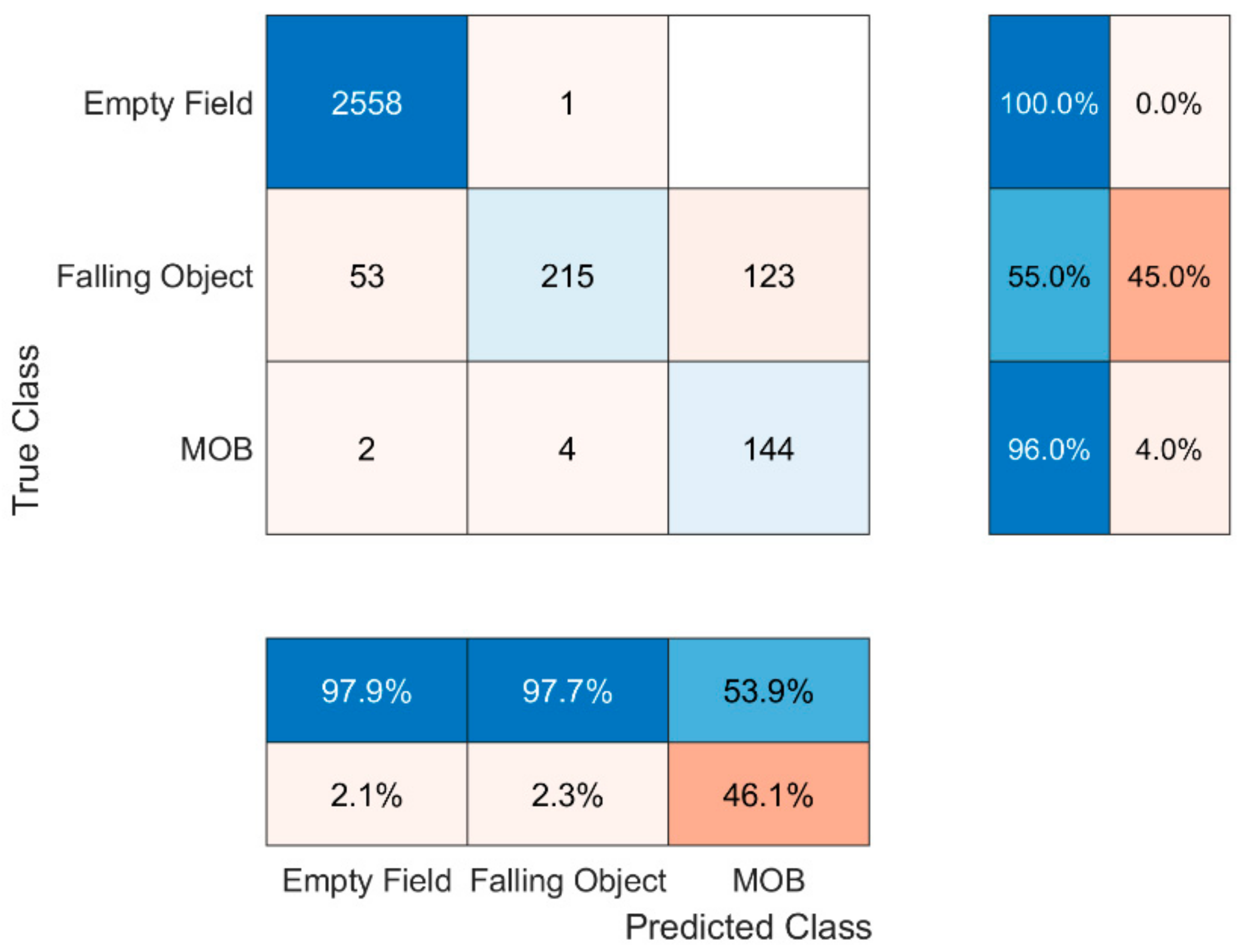
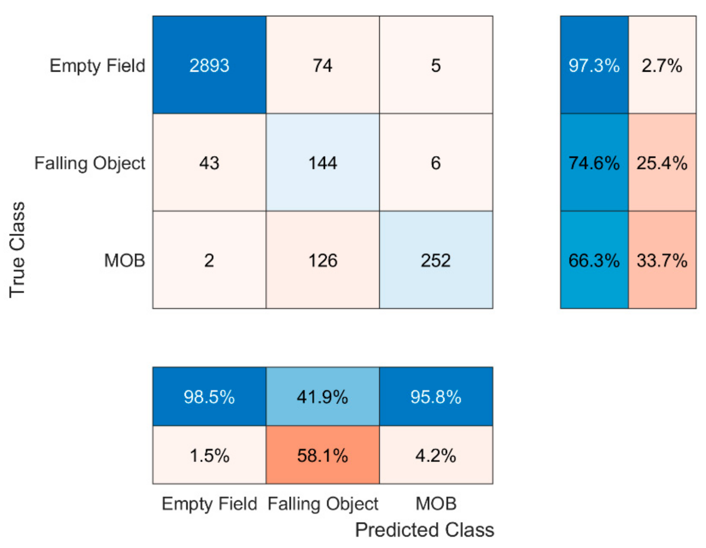
Figure 4 presents the confusion matrix depicting the results of the C1 fed using D1′s test set. Examining the results, it is clear that C1 never confuses the states ‘MOB’ with ‘clear field’ and vice versa. However, it is prone to confuse the fall of a human with the fall of an object. This could be interpreted as a logical outcome due to the similarity of the shape of some objects used during the measurements and the human body. On the other hand, some objects used in the experiment were too small leading the algorithm to predict that there is nothing falling when in reality there was an object falling.
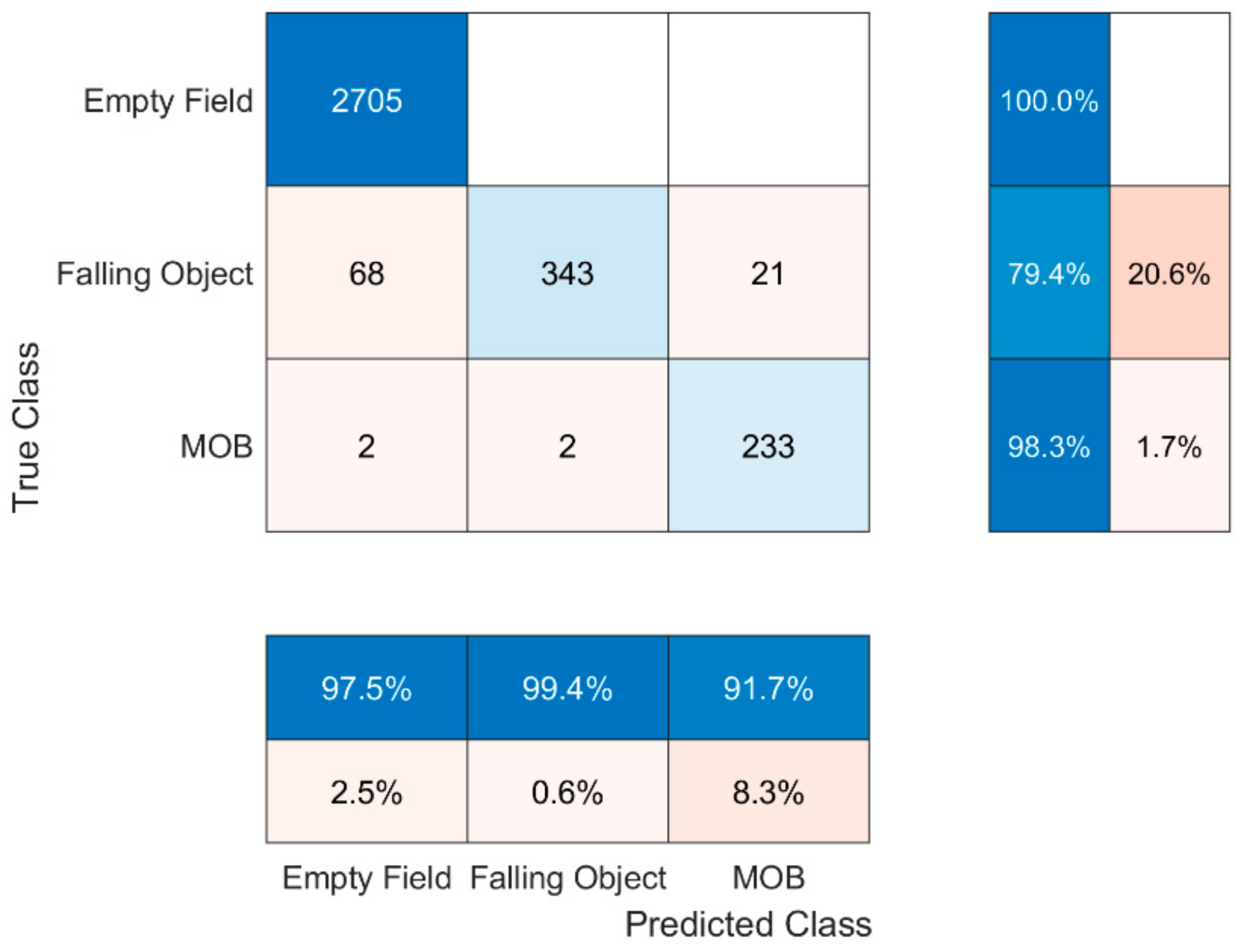
The same interpretations can also be inferred by looking the results of the C2 on D2′s test set in Figure 5. The only thing to be mentioned for the C2 is that it is more susceptible to predict MOB when the state is ‘falling object’. The latter could be a result of R2′s position; as opposed to R1, R2 was placed at a point where it was able to observe the falling objects the time when they had already achieved high velocity values, almost compared to the doll’s.
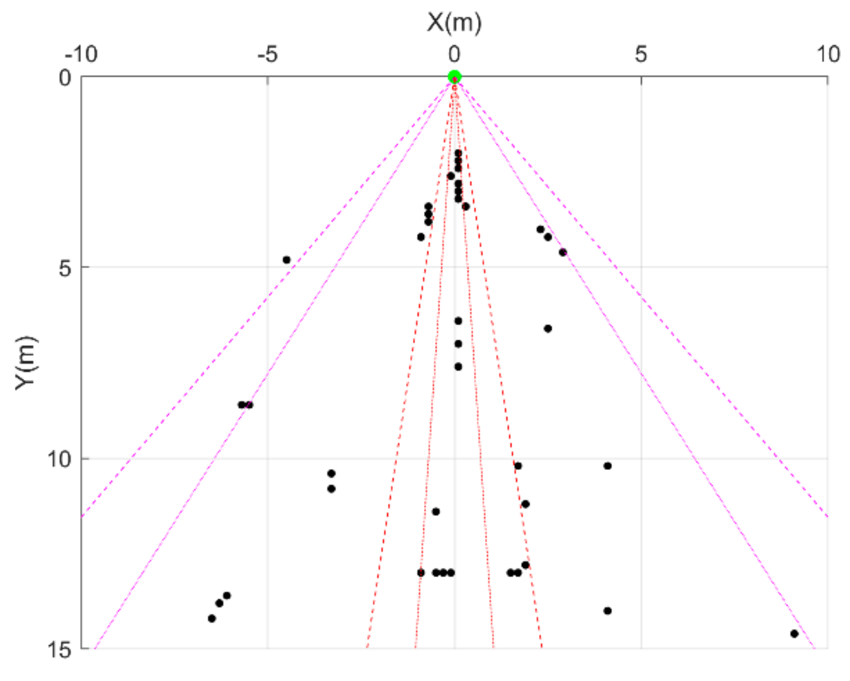
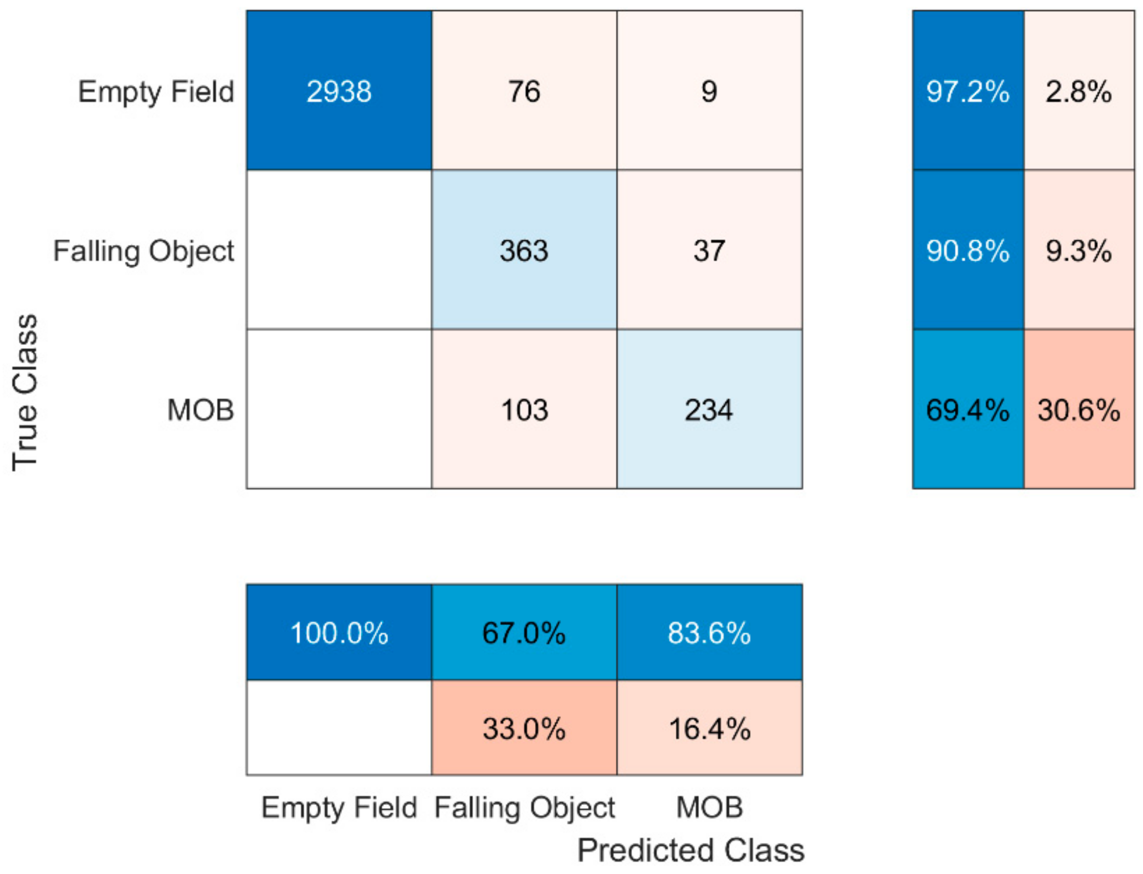
Nevertheless, the fusion of the radars, i.e., the joint information, seems to be promising. In that case, at each time point the joint decision is based on the worst-case decision made by the two radars. For instance, if R1 announces ‘Empty Field’ and R2 announces ‘MOB’, then the final decision will be ‘MOB’. Given this set-up, it seems that fusion can be more efficient in the ‘MOB’ state prediction, which is the most crucial one, by making the least faults. More precisely, the basis of fusion results in Table 3 which explains how fusion was implemented whereas Figure 6 portrays the confusion matrix of the fusion where 97.2% total accuracy achieved. However, while the fusion helped the algorithm to distinguish the states ‘Falling Object’ and ‘MOB’, it is still prone to confuse the states ‘Empty Field’ and ‘Falling Object’. Two possible reasons are to blame; firstly, many objects were too small leading the individual classifiers to predict that nothing was falling where the opposite was happening and, secondly, during the operation of the radars miscellaneous objects of the environment were being observed whereas ideally nothing should be. Indicatively for R1, which is placed 14 m above the ground facing downwards, the presence of substantial existing points that were constantly being observed is well understood by examining Figure 7 which represents the total observed points in a typical ‘Empty Field’ measurement scenario. In particular, the radar is placed at the point (0, 0) whereas the y axis represents the height from the radar point to the ground and the x axis the left–right direction, hence each point’s distance to the radar is . Moreover, further analysis revealed that their RCS values fluctuate between 0.1 and 0.9, information that also misleads the algorithm. Thus, mutual consideration of both the environmental existing points and the objects to be used during the training phase is highly encouraged in similar systems.
To conclude, using the aforementioned formulation for MWF1, Table 4 depicts the MWF1 scores and accuracies achieved by the C1, C2 and their fusion.
4.2. Support Vector Machines
SVMs are considered a powerful tool in classification problems due to their ability of finding a hyperplane of N-1 dimensions to divide the N-dimensional data in classes [17,18,19]. Therefore, a multiclass error-correcting output codes model containing SVM binary learners was used for training and predicting snapshots. The model was implemented in the MATLAB programming environment where the kernel of the learners was set to ‘Gaussian’ while the remaining options were left at their default values.
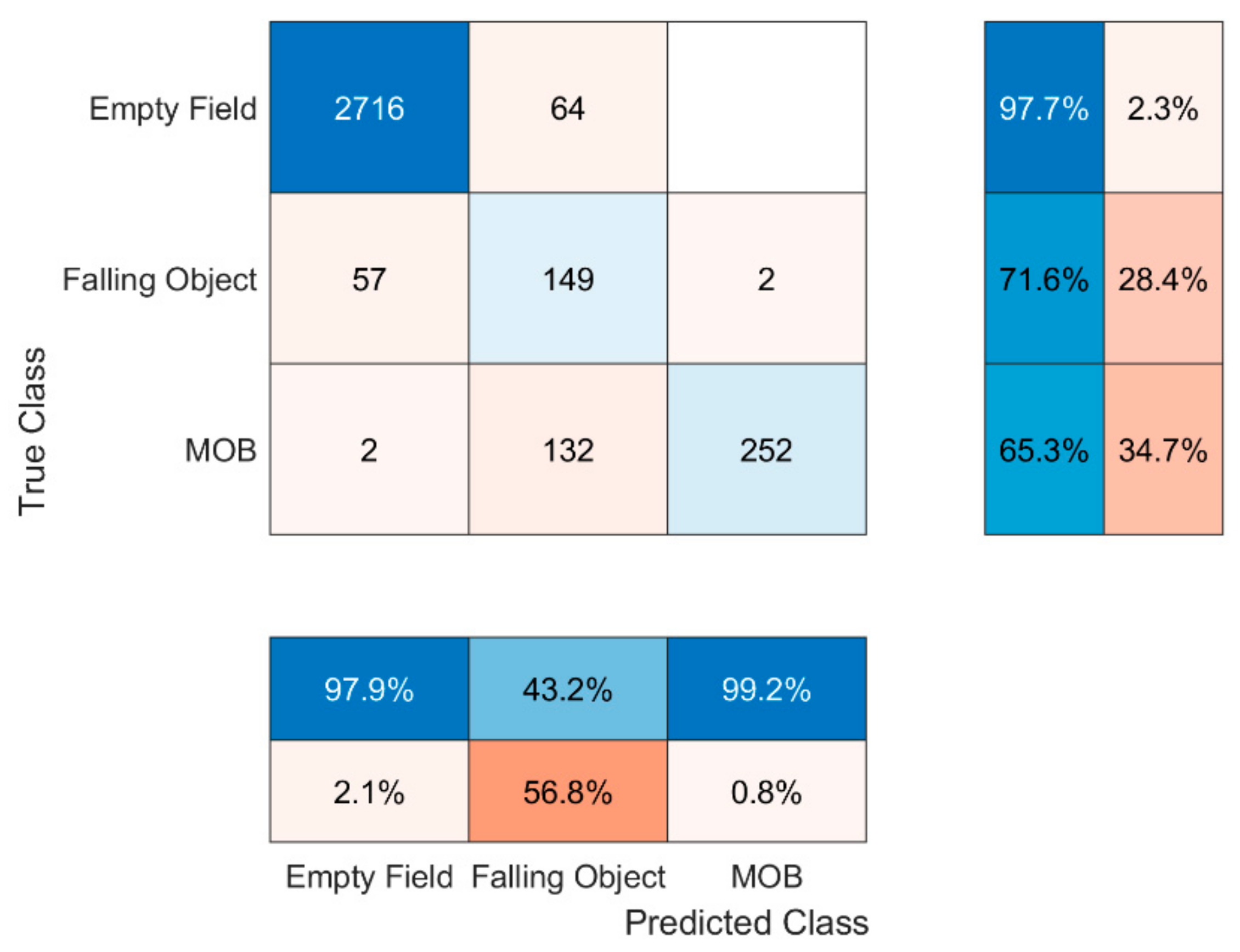
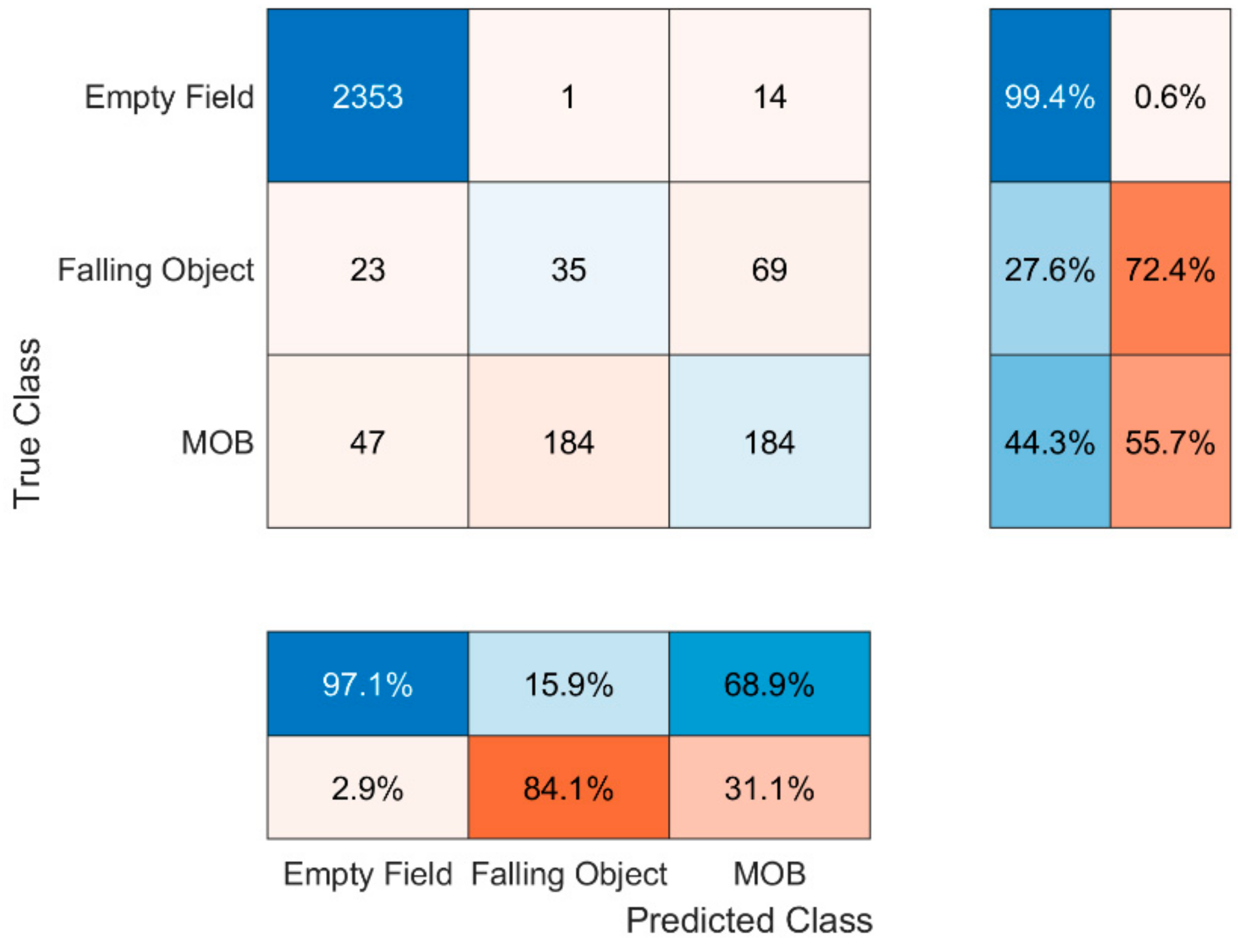
Examining Figure 8 depicting the confusion matrix of the sensors’ fusion, which is the optimal implementation, it is becoming clear that SVM algorithm tends to strongly confuse the states ‘MOB’ and ‘Falling Object’, thus making it insufficient for use. The latter is a logical outcome as neither C1 nor C2 are able to highly distinguish these two states. This can be seen with the aid of the confusion matrices of C1 and C2 presented in Figure 9 and Figure 10, respectively. One potential cause could be that the data is not linearly separable. Another reason could be that the dataset fed to the algorithm was imbalanced; the examples of ‘MOB’ state were being outnumbered by the examples of the other states. SVM is known to perform poorly in imbalanced sets. For comparison purposes, it is reported that the WMF1 score and accuracy of the fusion are 86.98% and 92.38%, respectively. The process followed to find these values is the same as in the case of random forest and thus it is omitted.
4.3. Naïve Bayes Classification
Another one strong classifier is the naïve Bayes which is probabilistic and selects the most suitable class for any example based on the maximum a posteriori decision rule [20,21]. However, to produce the best results the predictors have to be independent as this is the main assumption of the algorithm. The model was also implemented using the MATLAB programming environment whereas the options of the algorithm used left in their default values.
Similar findings as in the case of SVM can be seen in Figure 11, Figure 12 and Figure 13 where the confusion matrices of C1, C2 as well as the sensors’ fusion are depicted. By examining the results, it is becoming clear that even though the fusion improves the predicting performance, the tendency of the algorithm to confuse mostly the states ‘MOB’ and ‘Falling Object’ is making it also insufficient for use. The main reason this happens could be due to the feature independency assumption of the algorithm. In our scenarios the initial raw data was not fully independent; for instance, there was a dependency between the value of the coordinate on the y axis and the velocity of the falling objects. Nonetheless, it is mentioned that the WMF1 score and accuracy of the fusion are 90.83% and 94.90%, respectively. Finally, Table 5 depicts the aforementioned algorithm performances showing that the random forest classifier is the best option among the three. More research on different classifiers and techniques is encouraged in order for the results to be improved.
5. Conclusions
MOB incidents are of great interest as they are considered life-threatening situations where instant action needs to be taken. In the present work, an AI-aided system using radar sensors was implemented and proposed. Initially, the analysis of the system’s key characteristics is presented. Thereinafter, a thorough analysis of the AI preprocess flow was followed, and the work was concluded with the comparison of different AI algorithms. Numeric results were presented and interpreted throughout the paper in order to reveal insights and the main advantages and drawbacks of the system. As the main challenge of AI-aided systems is the dataset construction, implementations using more extensive and diverse datasets as well as different algorithmic approaches are left as future work. Moreover, extra measurement campaigns would allow the validation of the presented results under diverse water environments. Finally, the multiplicity and placement of the measurement equipment depends on the specific ship structure.
Author Contributions
V.T. implemented and executed the machine learning algorithms and wrote and edited the paper. V.T., C.K.A. and V.N. preprocessed and validated the dataset and the features that were inserted as input to the machine learning algorithms and edited the paper. P.S.B. and A.G.K. had the initial idea for the implementation of this paper. P.S.B. and A.G.K. also edited, reviewed and supervised the paper. All authors have read and agreed to the published version of the manuscript.
Funding
This research was cofinanced by the European Regional Development Fund of the European Union and Greek national funds through the Operational Program Competitiveness, Entrepreneurship and Innovation, under the call RESEARCH—CREATE—INNOVATE (project code: T1EDK-01169, project name: MHTIS).
Conflicts of Interest
The authors declare no conflict of interest.
References
- Kumar, Y.; Kaur, K.; Singh, G. Machine Learning Aspects and its Applications towards Different Research Areas. In Proceedings of the 2020 International Conference on Computation, Automation and Knowledge Management (ICCAKM), Dubai, United Arab Emirates, 9–10 January 2020; pp. 150–156. [Google Scholar] [CrossRef]
- Chen, Y.; Lin, Z.; Zhao, X.; Wang, G.; Gu, Y. Deep Learning-Based Classification of Hyperspectral Data. IEEE J. Sel. Topics Appl. Earth Observ. Remote Sens. 2014, 7, 2094–2107. [Google Scholar] [CrossRef]
- Zhao, R.; Zhang, H.; Lu, J.; Li, C.; Zhang, H. A New Machine Learning Method based on PCA and SVM. In Proceedings of the 2006 International Conference on Computational Intelligence and Security, Guangzhou, China, 3–6 November 2006; pp. 187–190. [Google Scholar] [CrossRef]
- Hou, R.; Chang, H.; Ma, B.; Shan, S.; Chen, X. Cross Attention Network for Few-Shot Classification. arXiv 2019, arXiv:1910.07677. [Google Scholar]
- Sevin, A.; Bayilmis, C.; Erturk, İ.; Ekiz, H.; Karaca, A. Design and implementation of a man-overboard emergency discovery system based on wireless sensor networks. Turk. J. Electr. Eng. Comput. Sci. 2016, 24, 762–773. [Google Scholar] [CrossRef]
- Örtlund, E.; Larsson, M. Man Overboard Detecting Systems Based on Wireless Technology; Chalmers Open Digital Repository: Gothenburg, Sweden, 2018. [Google Scholar]
- Sheu, B.; Yang, T.; Yang, T.; Huang, C.; Chen, W. Real-time Alarm, Dynamic GPS Tracking, and Monitoring System for Man Overboard. Sens. Mater. 2020, 32, 197. [Google Scholar] [CrossRef] [Green Version]
- Katsamenis, I.; Protopapadakis, E.; Voulodimos, A.; Dres, D.; Drakoulis, D. Man overboard event detection from RGB and thermal imagery. In Proceedings of the 13th ACM International Conference on PErvasive Technologies Related to Assistive Environments, Corfu, Greece, 30 June–3 July 2020. [Google Scholar]
- Feraru, V.A.; Andersen, R.E.; Boukas, E. Towards an Autonomous UAV-based System to Assist Search and Rescue Operations in Man Overboard Incidents. In Proceedings of the 2020 IEEE International Symposium on Safety, Security, and Rescue Robotics (SSRR), Abu Dhabi, United Arab Emirates, 4–6 November 2020; pp. 57–64. [Google Scholar] [CrossRef]
- Lygouras, E.; Santavas, N.; Taitzoglou, A.; Tarchanidis, K.; Mitropoulos, A.; Gasteratos, A. Unsupervised Human Detection with an Embedded Vision System on a Fully Autonomous UAV for Search and Rescue Operations. Sensors 2019, 19, 3542. [Google Scholar] [CrossRef] [PubMed] [Green Version]
- Wang, Q.; Wang, S.; Gong, M.; Wu, Y. Feature Hashing for Network Representation Learning. In Proceedings of the Twenty-Seventh International Joint Conference on Artificial Intelligence, Stockholm, Sweden, 13–19 July 2018; pp. 2812–2818. [Google Scholar]
- Wang, S.; Gong, M.; Wu, Y.; Zhang, M. Multi-objective optimization for location-based and preferences-aware recommendation. Inf. Sci. 2020, 513, 614–626. [Google Scholar]
- Tin Kam, H. Random decision forests. In Proceedings of the 3rd International Conference on Document Analysis and Recognition, Montreal, QC, Canada, 14–16 August 1995; Volume 1, pp. 278–282. [Google Scholar] [CrossRef]
- Piryonesi, S.M.; El-Diraby, T.E. Role of Data Analytics in Infrastructure Asset Management: Overcoming Data Size and Quality Problems. J. Transp. Eng. Part B Pavements 2020, 146, 04020022. [Google Scholar] [CrossRef]
- Piryonesi, S.M.; El-Diraby, T.E. Using Machine Learning to Examine Impact of Type of Performance Indicator on Flexible Pavement Deterioration Modeling. J. Infrastruct. Syst. 2021, 27, 04021005. [Google Scholar] [CrossRef]
- Opitz, J.; Burst, S. Macro F1 and Macro F1. arXiv 2019, arXiv:1911.03347. [Google Scholar]
- Cortes, C.; Vapnik, V. Support-vector networks. Mach. Learn. 1995, 20, 273–297. [Google Scholar] [CrossRef]
- Ben-Hur, A.; Horn, D.; Siegelmann, H.; Vapnik, V. Support Vector Clustering. J. Mach. Learn. Res. 2001, 2, 125–137. [Google Scholar] [CrossRef]
- Boser, B.E.; Guyon, I.M.; Vapnik, V.N. A Training Algorithm for Optimal Margin Classifier. In Proceedings of the Fifth Annual ACM Workshop on Computational Learning Theory, Pittsburgh, PA, USA, 27–29 July 1992. [Google Scholar]
- McCallum, A. Graphical Models, Lecture2: Bayesian Network Represention. Retrieved 2019, 22. [Google Scholar]
- Zhang, H. The Optimality of Naive Bayes. In Proceedings of the Seventeenth International Florida Artificial Intelligence Research Society Conference, Miami Beach, FL, USA, 12–14 May 2004. [Google Scholar]
Figure 1.
Radar FoV.

Figure 2.
System architecture.

Figure 3.
Human shaped doll.

Figure 4.
C1′s confusion matrix.

Figure 5.
C2′s confusion matrix.

Figure 6.
Fusion’s confusion matrix.

Figure 7.
Total points observed from R1 in a typical ‘Empty Field’ measurement scenario.

Figure 8.
Fusion’s confusion matrix.

Figure 9.
C1′s confusion matrix.

Figure 10.
C2′s confusion matrix.

Figure 11.
Fusion’s confusion matrix.

Figure 12.
C1′s confusion matrix.

Figure 13.
C2′s confusion matrix.


Table 1.
Technical characteristics of the radar sensors (the azimuth angle is measured on a plane parallel to the building facade whereas the elevation angle is measured on a plane perpendicular to the building facade).
Table 1.
Technical characteristics of the radar sensors (the azimuth angle is measured on a plane parallel to the building facade whereas the elevation angle is measured on a plane perpendicular to the building facade).
| Continental ARS 408-21 Long Range Radar Sensor | |
|---|---|
| Operating frequency | 76–77 GHz |
| Near field distance range | 0.20–70/100 m |
| Near field azimuth angle field of view (FoV) | ±60° |
| Near field elevation angle field of view (FoV) | ±20° |
| Far field distance range | 0.20–250 m |
| Far field azimuth angle field of view (FoV) | ±9° |
| Far field elevation angle field of view (FoV) | ±14° |
| Near field distance measuring accuracy | ±0.10 m |
| Far field distance measuring accuracy | ±0.40 m |
| Velocity range | −400–200 km/h |
| Velocity measuring accuracy | 0.1 km/h |
Table 2.
Features made up the dataset fed to ML algorithms.
| Features | Derivation |
|---|---|
| Mean(Φ) | Mean value of all points’ Φ value in the snapshot |
| Variance(Φ) | Variance of all points’ Φ value in the snapshot |
| Skewness(Φ) | Skewness of all points’ Φ value in the snapshot |
| Kurtosis(Φ) | Kurtosis of all points’ Φ value in the snapshot |
| Entropy(Φ) | Entropy of all points’ Φ value in the snapshot |
| RMS(Φ) | Root mean square of all points’ Φ value in the snapshot |
| Impulse factor(Φ) | Impulse factor square of all points’ Φ value in the snapshot |
| Median(Φ) | Median of all points’ Φ value in the snapshot |
| Mad(Φ) | Median absolute deviation of all points’ Φ value in the snapshot |
| Iqr(Φ) | Interquartile range of all points’ Φ value in the snapshot |
| Number of Points | Number of points in the snapshot |
| meanDistMovPoints | Mean distance of all the points |
| meanVelDiff | Mean velocity difference between consecutive snapshots |
| meanAccDiff | Mean acceleration difference between consecutive snapshots |
Table 3.
Decisions taken from the fusion of the radar sensors.
| C1 | C2 | Joint Decision |
|---|---|---|
| Empty Field | Empty Field | Empty Field |
| Empty Field | Falling Object | Falling Object |
| Empty Field | MOB | MOB |
| Falling Object | Empty Field | Falling Object |
| Falling Object | Falling Object | Falling Object |
| Falling Object | MOB | MOB |
| MOB | Empty Field | MOB |
| MOB | Falling Object | MOB |
| MOB | MOB | MOB |
Table 4.
Most useful metrics of the classifiers and their fusion used for comparison among different approaches.
Table 4.
Most useful metrics of the classifiers and their fusion used for comparison among different approaches.
| C1 | C2 | Fusion | |
|---|---|---|---|
| F1 Empty Field | 99.81% | 98.92% | 98.72% |
| F1 Falling Object | 92.08% | 70.38% | 88.29% |
| F1 MOB | 84.66% | 69.06% | 94.91% |
| WMF1 | 95.62% | 89.71% | 94.68% |
| Accuracy | 97.69% | 94.10% | 97.24% |
Table 5.
Comparison of the algorithms’ WMF1 score and accuracy.
| Algorithm | WMF1 Score (Fusion) | Accuracy (Fusion) | Comments |
|---|---|---|---|
| Random forest | 94.68% | 97.24% | Sufficient for use |
| SVM | 86.98% | 92.38% | Insufficient for use due to its high tendency of confusion the states ‘MOB’ and ‘Falling Object’ |
| Naïve Bayes | 90.83% | 94.90% | Insufficient for use due to its high tendency of confusion the states ‘MOB’ and ‘Falling Object’ |
Publisher’s Note: MDPI stays neutral with regard to jurisdictional claims in published maps and institutional affiliations. |
© 2021 by the authors. Licensee MDPI, Basel, Switzerland. This article is an open access article distributed under the terms and conditions of the Creative Commons Attribution (CC BY) license (https://creativecommons.org/licenses/by/4.0/).
Share and Cite
MDPI and ACS Style
Tsekenis, V.; Armeniakos, C.K.; Nikolaidis, V.; Bithas, P.S.; Kanatas, A.G. Machine Learning-Assisted Man Overboard Detection Using Radars. Electronics 2021, 10, 1345. https://0-doi-org.brum.beds.ac.uk/10.3390/electronics10111345
AMA Style
Tsekenis V, Armeniakos CK, Nikolaidis V, Bithas PS, Kanatas AG. Machine Learning-Assisted Man Overboard Detection Using Radars. Electronics. 2021; 10(11):1345. https://0-doi-org.brum.beds.ac.uk/10.3390/electronics10111345
Chicago/Turabian StyleTsekenis, Vasileios, Charalampos K. Armeniakos, Viktor Nikolaidis, Petros S. Bithas, and Athanasios G. Kanatas. 2021. "Machine Learning-Assisted Man Overboard Detection Using Radars" Electronics 10, no. 11: 1345. https://0-doi-org.brum.beds.ac.uk/10.3390/electronics10111345
Note that from the first issue of 2016, this journal uses article numbers instead of page numbers. See further details here.