
Zone-Agnostic Greedy Taxi Dispatch Algorithm Based on Contextual Matching Matrix for Efficient Maximization of Revenue and Profit


Department of Computer Engineering, Hongik University, Seoul 04066, Korea
*
Author to whom correspondence should be addressed.
Electronics 2021, 10(21), 2653; https://0-doi-org.brum.beds.ac.uk/10.3390/electronics10212653
Submission received: 2 October 2021
/
Revised: 27 October 2021
/
Accepted: 28 October 2021
/
Published: 29 October 2021
(This article belongs to the Special Issue AI-Based Transportation Planning and Operation, Volume II)
Abstract
:This paper addresses the taxi fleet dispatch problem, which is critical for many transport service platforms such as Uber, Lyft, and Didi Chuxing. We focus on maximizing the revenue and profit a taxi platform can generate through the dispatch approaches designed with various criteria. We consider determining the proportion of taxi fleets to different destination zones given the expected rewards from the future states following the distribution decisions learned through reinforcement learning (RL) algorithms. We also take into account more straightforward greedy algorithms that look ahead fewer decision time steps in the future. Our dispatch decision algorithms commonly leverage contextual information and heuristics using a data structure called Contextual Matching Matrix (CMM). The key contribution of our paper is the insight into the trade-off between different design criteria. Primarily, through the evaluation with actual taxi operation data offered by Seoul Metropolitan Government, we challenge the natural expectation that the RL-based approaches yield the best result by showing that a lightweight greedy algorithm can have a competitive advantage. Moreover, we break the norm of dissecting the service area into sub-zones and show that matching passengers beyond arbitrary boundaries generates significantly higher operating income and profit.
1. Introduction
Assigning taxis or drivers to passengers is a critical decision problem for many transport service platforms such as Uber, Lyft, and Didi Chuxing that serve millions of users daily. The effectiveness of these taxi platforms is evaluated in terms of the percentage of the taxi-to-passenger match success rate and a passenger’s wait time, which eventually determine the operating income and profit. This paper focuses on the maximization of the revenue and profit a taxi platform can generate through a variety of taxi dispatch approaches designed with the following criteria.
First, we can consider the probable information from the future states following dispatch actions. We can employ reinforcement learning (RL) [1] techniques that learn to update the value of an action at a particular state after computing the reward from the distant future. An alternative is to craft a simpler greedy algorithm that looks ahead fewer decision time steps.
Second, the service area can be divided into high-demand sub-area clusters, a grid of square or hexagonal cells, or administrative divisions. We can opt to match a taxi with passengers only within the same zone, which is a prevalent method in most of the recent works [2,3,4] implemented. Alternatively, we can have a zone-agnostic approach that does not limit the assignment of the taxis to the passenger calls within an arbitrary boundary.
Third, for the zone-sensitive assignment, we can consider the proportion of taxi fleets allocated to destination zones before matching taxis with passengers individually. With a global view of the demands, the platform can direct portions of its limited number of taxis towards different destination zones. This approach attempts to prevent the taxis from potentially making sub-optimal decisions due to the lack of a view of global demands. We apply RL techniques to determine the best fleet distribution among destination zones. For a zone-agnostic approach, determining the fleet proportion is unnecessary.
The dispatch approaches we devise in this paper commonly leverage contextual information and heuristics using a data structure called the Contextual Matching Matrix (CMM) [5]. Our approach utilizes CMM to match a taxi and a passenger given the distance between the two, the distance between the pickup location and final destination, and the estimated demands at the drop-off area. The CMM usage differs from the previous approaches with plain decision criteria such as first-come-first-serve matching with a queue of calls [6,7] and matching closest passenger first [8,9,10]. With CMM, our approaches search for a dispatch action that reduces the passenger pickup cost and yields a high taxi utilization rate by matching taxis to the passengers aiming to reach the high-demand area.
The critical contribution of this paper is the insight into the trade-off between the various design criteria through the evaluation based on the actual taxi operation data provided by the Seoul Metropolitan Government. Primarily, we challenge the natural expectation that the RL-based approach of determining the fleet distribution is likely to yield the highest revenue and profit. We examine whether a fast and more straightforward greedy algorithm with CMM can be a more viable and practical solution for the taxi platforms operating in the field. In addition, contrary to the conventional approach based on the dissection of the service area, we show that not considering the zone information generates a much better result.
2. Related Works
In this section, we present relevant works on taxi dispatching systems.
2.1. Taxi Dispatching Systems
With accurate GPS receivers and fast wireless communication interfaces, traditional taxi management systems are transforming to become more efficient and profitable [11]. Previous works recommend that drivers pass through the routes where potential passengers might exist [12] or travel to high-demand spots [13]. Most recent ride-hailing platforms either match a driver to the closest passenger call [8,9,10] or use queueing strategies for first-come-first-served dispatching [6,7]. Zhou et al. proposed a model which dispatches taxis in such a way that demands and supplies are balanced based on demand prediction [3]. Furthermore, Xu et al. used a recurrent neural network (RNN) and captured complex spatio-temporal features to predict taxi demand [14]. Yang et al. studied the demand and supply equilibrium of taxi services regulating the fare system and fleet size [15]. Conventionally, automated taxi dispatching systems try to minimize passenger wait time and taxi idle time or match the closest vacant taxi to a given order [9,10,16,17]. Zhang et al. used the combinatorial optimization [18] technique to improve the probability of successful matching [19]. Park et al. exploit the optimal price to match taxis with passengers and simultaneously maximize cumulative revenue [5]. Similarly, Zheng et al. studied optimal pricing [20], and Zhao et al. analyzed passengers’ preferences [21].
Recent approaches divide a region into a grid of cells and match vacant taxis with the passenger calls that take place within the same cell to maximize the driver’s profit and the match rate [2,3]. Liu et al. proposed a road-connectivity-aware zone that was formed by clustering the road network graph as opposed to having a grid of rectangular and hexagonal cells [4]. Based on the road connectivity and the travel cost, the optimal dispatch method was computed. This paper does not restrict the matching to the passenger calls only within a particular service zone; we study the approach of matching taxis to passengers across the zone boundaries as well.
2.2. Reinforcement Learning
The recent extraordinary advancement of machine learning algorithms has sparked the interest of researchers studying the taxi dispatch problem. Noticeably, the investigation of the application of reinforcement learning (RL) [1] has been active [22,23]. With RL using artificial neural networks, the complex state transition patterns and the most rewarding actions in a given state can be learned [24]. Considering the far-sighted future, using RL can be helpful for the taxi dispatch problem since a short-sighted decision by the drivers may not guarantee a high profit in the long term. For instance, a driver who chooses to pick up the closest passenger may end up in a drop location that remains vacant for a long time due to a lack of subsequent orders. The multi-agent methodology is used in several traffic problems. For ride-sharing scenarios, Li et al. proposed a multi-agent reinforcement learning solution addressing order dispatch problems in a large-scale city [25]. De et al. also used multi-agent reinforcement learning for ride-sharing using QMIX [26]. Multi-agent RL techniques were applied to the problem of taxi fleet dispatch as well [2,3,27]. In these works, taxis within the same pre-defined zone take actions based on the shared state information. In another multi-agent RL approach, every taxi learns to decide actions independently without shared state information [28,29]. In this paper, we employ the Deep Q-Network [24] particularly to determine the optimal proportion of taxis to be distributed among different zones before matching the taxis with individual passenger calls. However, RL for the taxi dispatch problem relies on a weak Markov decision process model where the dispatch action may not be the direct cause of the succeeding state, such as the sudden rise of the passenger demand at the drop-off location. Such RL can be prone to learn sub-optimal decisions. Therefore, we devised a more uncomplicated, novel, greedy method with a slight look-ahead to the future that runs faster and chooses more profitable actions.
3. Modeling the Taxi Dispatch Problem
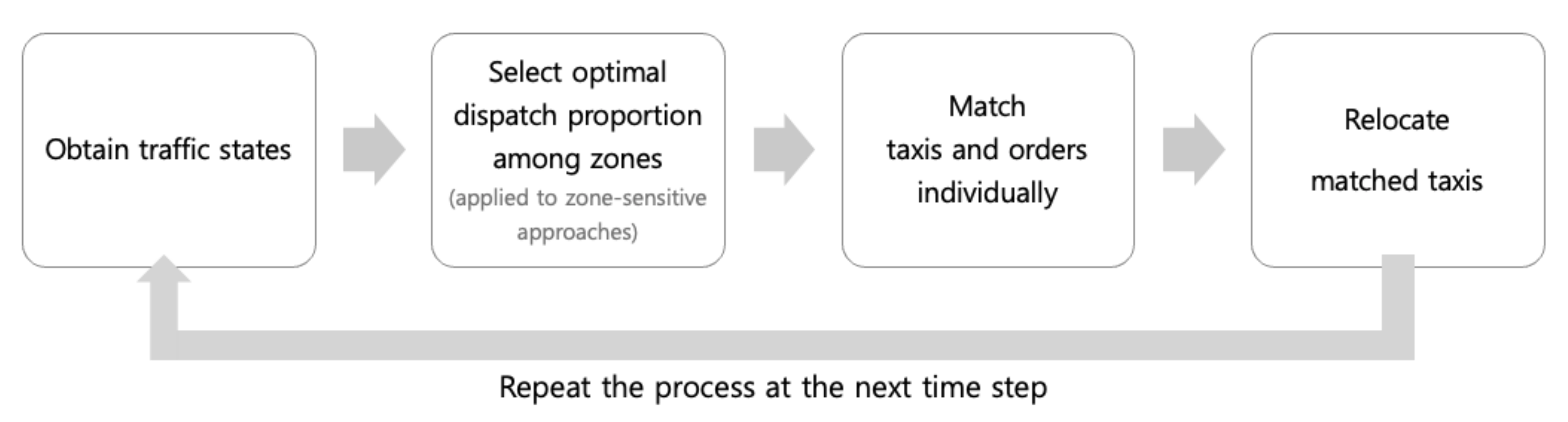
In this section, we model the taxi dispatch process (Figure 1). First, we obtain information on how the idle taxis and the customer demands are spatially distributed. Second, we determine the optimal proportion of the taxi fleet dispatched to different zones in the case that the service area is dissected. For each pool of taxis with a certain portion, we match the taxis in the pool with individual passenger calls. After drop-off, taxis are added to the pool of idle taxis waiting for the next dispatch decision. Every 30 s, the dispatch process restarts for the currently available vacant taxis. Our objective is to retrieve the optimal match between idle taxis and passengers to maximize revenue and profit.
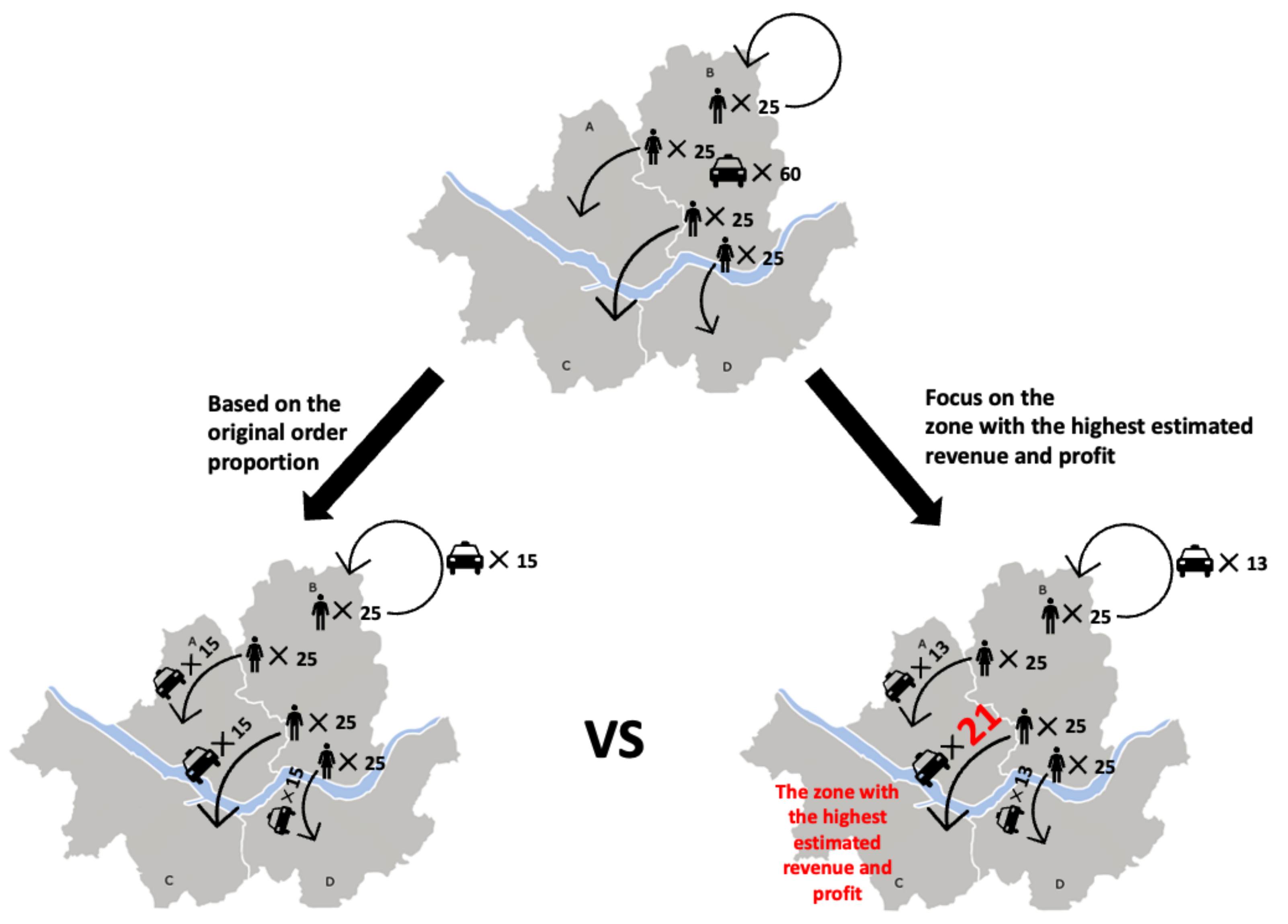
When demand is higher than the supply in a departure zone, there will undoubtedly be mismatched demand. Therefore, minimizing the mismatch rate between passenger orders and taxis is critical to pursue high revenue and profit. For example, as shown in Figure 2, a naïve division of the taxi in proportion to the passenger demands to different destination zones may yield sub-optimal results. We can predict the situation in the drop-off zone through simulation and assign more taxis to the destination zone that is expected to offer more revenue and profit-generation opportunities. To determine the optimal proportions, we divide the service area into multiple sub-areas.
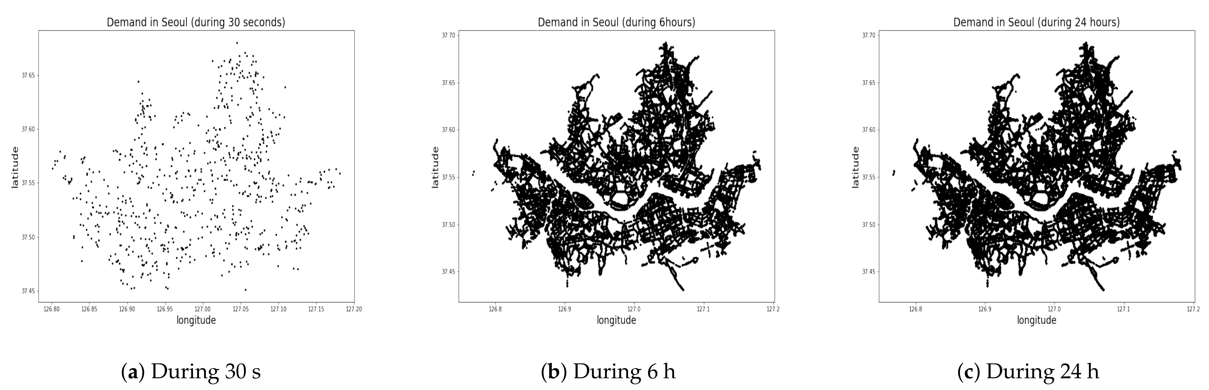
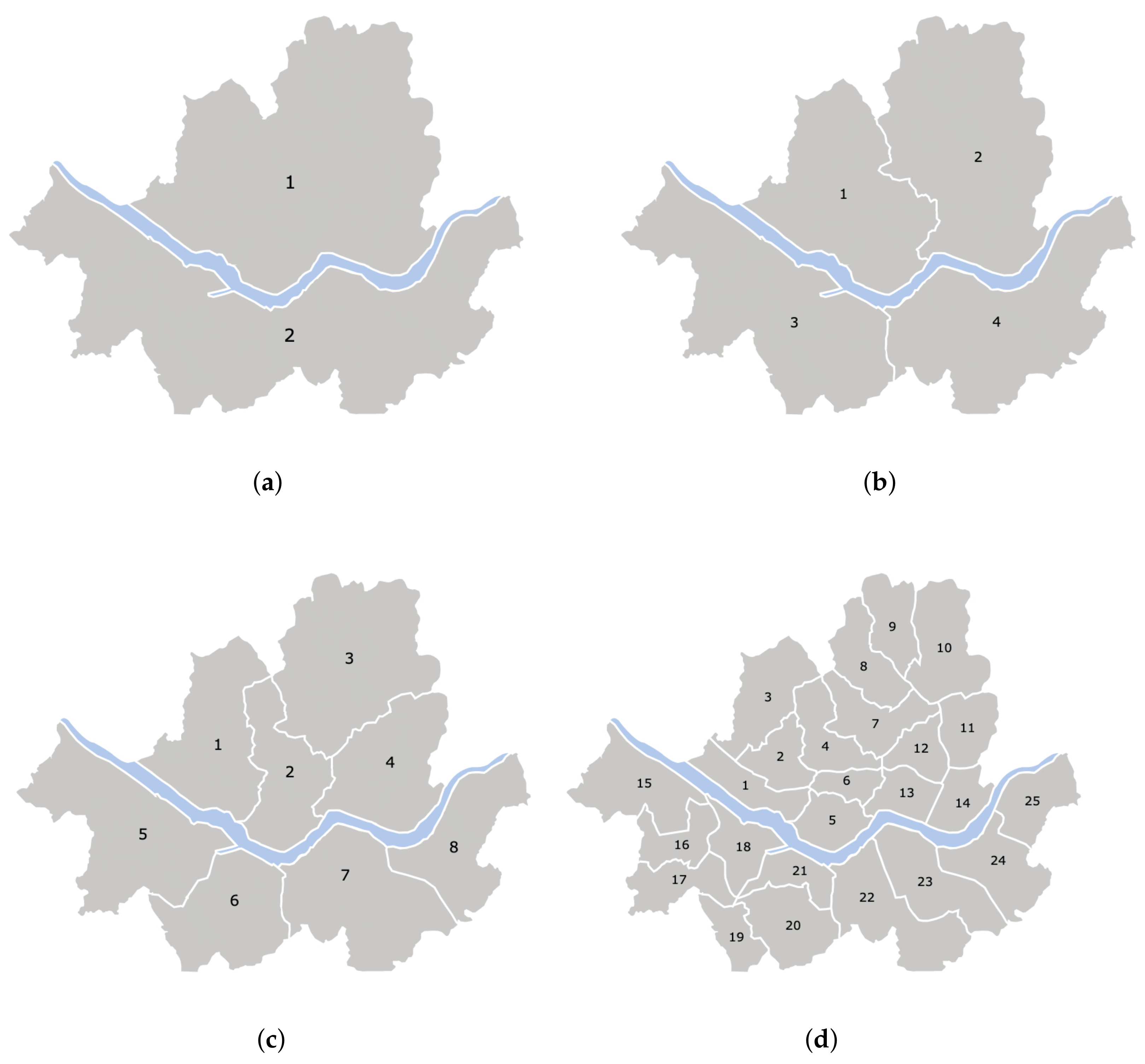
Existing works divide the service region into a grid of rectangular or hexagonal cells [2,3,30] or cluster high passenger demand spots [4,5] using algorithms such as K-means clustering [31] or the density-based spatial clustering of applications with noise (DBSCAN) algorithms [32,33]. No meaningful cluster can be identified if spots are scattered uniformly all across the region, as shown in the distribution of passenger calls during 30 s, 10 min, 24 h in Seoul, South Korea (Figure 3). No more than two clusters are detected around the Han River in the middle of the area. In this work, we chose to divide the service region into 2 to 25 administrative divisions (zones) as shown in Figure 4, which is similar to the grid-based approaches implemented in [2,3,30]. We model the fleet management method that ignores the divisions and matches passenger calls with vacant taxis on a point-to-point basis.
It is infeasible for a single decision-making agent to determine the optimal proportion of fleets distributed among all different zones due to the explosive number of cases to explore. For example, the number of possible proportions of taxis for each destination zone is . A single decision-making agent has to choose the optimal proportion among proportions where is the number of zones. If is 25 and is 26, a single decision-making agent has to search for the optimal proportions among proportions. When we handle this situation using a multi-agent approach, the agent of each zone chooses a proportion distribution from distributions. The action space that multi-agents explore concurrently is significantly lower than the action space explored by the system with a single global agent. Hence, we opt to have a separate dispatch decision process run by an independent agent within each zone.
The revenue and the profit of the taxi fleet management system are computed according to Equations (1) and (2), respectively. is the total distance in kilometers driven by the taxis to take the passengers from their origins to the desired destinations. Taxis charge 100 Korean Won for every 132 m. is the total distance in kilometers driven by taxis to pick up the passengers. Picking up a passenger also costs 100 Korean Won for every 132 m. A taxi can move 400 m each 30 s in this setting. Since idle taxis miss the opportunity cost of moving 400 m every 30 s with passengers on board, the last term of the profit in Equation (2) is the opportunity cost of idle taxis. We set the smallest wait time unit to 30 s. Any unmatched taxis have to wait 30 s until the next decision-making step recurs. A naïve real-time system would implement the first-come-first-served approach for each taxi agent. However, such an approach is likely to yield sub-optimal values due to selfish agents that lack global information. The 30 s wait time allows the coordination platform to make a globally optimal dispatch decision. Taxis and passengers more than 8 kilometers apart are not matched to avoid the passenger wait time becoming longer than 10 min. Definitions of notations used in this paper are listed in Table 1.
A taxi matched with a passenger becomes idle in the drop-off (destination) zone () after moving 400 m every 30 s. The travel time to the destination zone is shown in Equation (3), where is the distance between the origin of the ith matching passenger to the destination, and 0 to 5 min of extra time is randomly added. In addition, is the time to pick up the ith matched passenger.
At every periodic iteration of the dispatch process, a taxi falls into one of the following states: (1) matched with a passenger and on the way to the passenger; (2) matched with a passenger and driving the passenger to ; and (3) remaining idle if unmatched.
4. Methodology
This paper offers five distinctive methods that can be distinguished by the combination of five critical criteria as shown in Table 2. First, a method can opt to match taxis only with the passengers that are located within the same zone. Second, a method may determine the proportion of taxis to be dispatched to different zones. Third, suppose a method takes into account the future states; in that case, it is either far-sighted by looking ahead unlimited future states or is myopic by forecasting the state after D future decision process iterations at most. A method can be completely greedy by not foreseeing the future states at all. Fourth, a method may favor a dispatch decision that leads to the spatial distribution of the taxis at the drop-off location matching closely to the spatial distribution of new passenger calls. Devising each method and unraveling the trade-offs through empirical evaluation as discussed in Section 5 is one of the novel contributions of this paper.
In the methods used to determine proportions, as mentioned in Section 3, it is necessary to constrain the task of determining the ratios between the number of taxis that are to be sent to different zones, as the possible ratios to be considered is unlimited. Unlike previous works [2,3,27] that allow individual taxis to make their own decision, we assign a decision-making agent for each zone. The agent for each zone determines the proportion of the taxis to be dispatched to other zones. The agent employs a 10% surplus to the proportion for every zone. The agent also considers taxi fleets to be distributed strictly in proportion to the demand of destination zones. Hence, the number of distributions that can be determined by the agents is .
4.1. CMM (Contextual Matching Matrix)
The first method to present adapts the work by Park et al., which uses a contextual matching matrix (CMM) to decide the optimal taxi fare dynamically [5]. denotes a row of the ith passenger call. As mentioned earlier, idle taxis with a passenger-to-driver distance of over 8 km are excluded from computing the match likelihood. Hence, each element of the PD matrix is defined in Equation (4). Each element of is a normalized distance from the passenger to an idle taxi, where is defined in Equation (5).
Every term in is multiplied by and to compute the match likelihood , as shown in Equation (6).
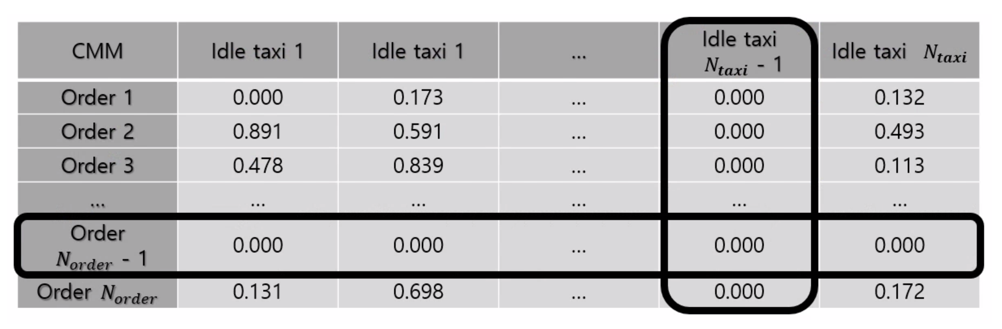
Once the computation according to Equation (6) is completed for all rows, we execute Algorithm 1 to retrieve matched pairs of passengers and taxis. We find the highest in , and we mark the ith passenger and the jth taxi as matched. Then, we cross them out by setting every term of both and to zero as shown in Figure 5. In the next iteration, the jth taxi is not redundantly considered to match other passengers, even though the initial computation result shows that the jth taxi matches with another passenger with the highest value of all other taxis. We repeat this iteration until becomes free of non-zero values. Removing the taxi from consideration immediately upon matching helps with the expedition of the algorithm as well. Matching based on CMM is the basis for other dispatch decision methods, as presented below.
| Algorithm 1: Making match with Contextual Matching Matrix (CMM) |
 |
4.2. M-Greedy
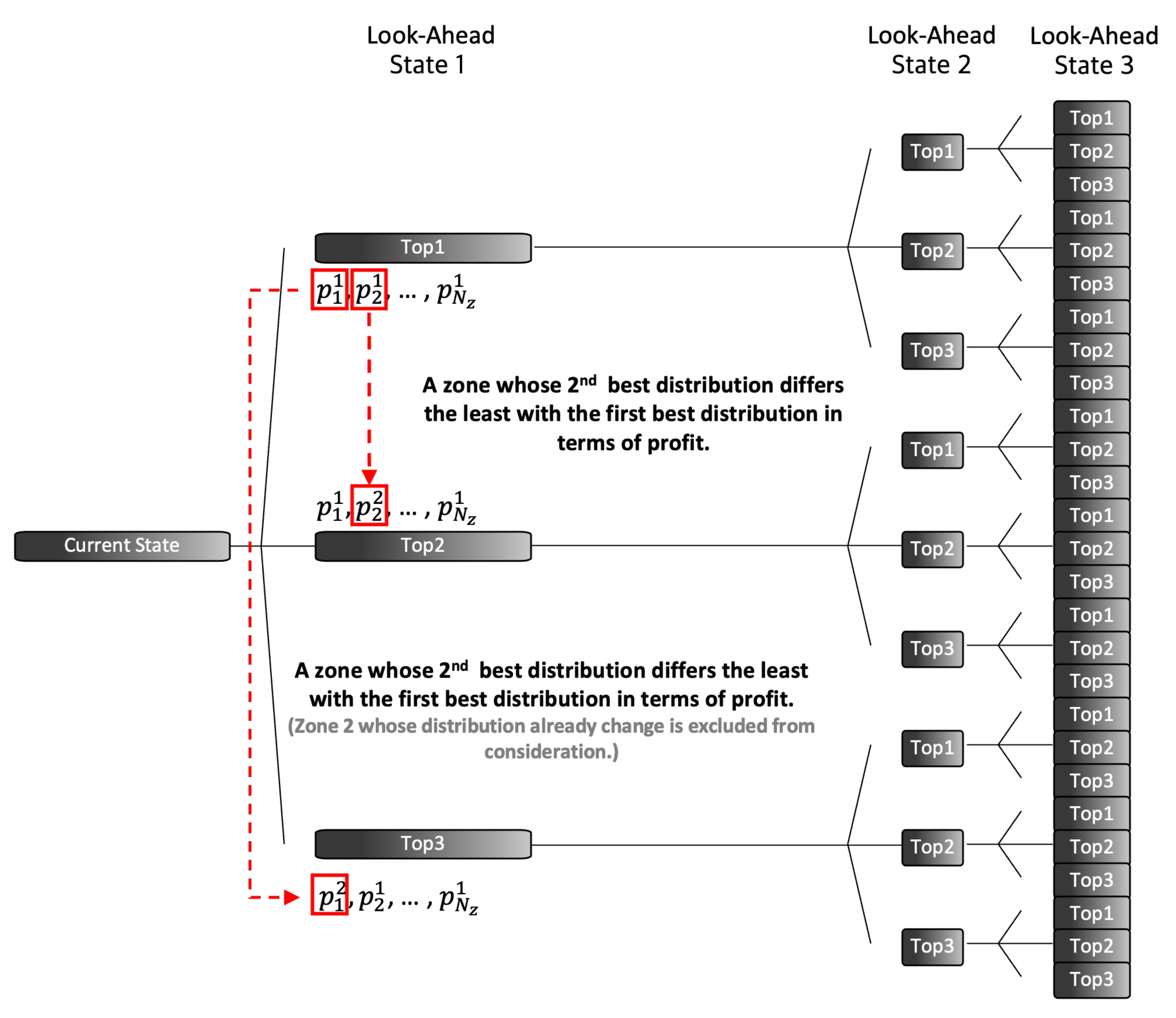
The CMM approach presented in Section 4.1 does not take the future further than the next immediate state into account. Thus, we devised M-Greedy, which extends CMM to look ahead D future states. We adapted CMM to look ahead myopically as follows. At the beginning of every decision process, we chose the top-k fleet distributions out of all possible cases. M-Greedy repeats this top-k selection process at each follow-up state. As shown in Figure 6, M-Greedy is myopic as we set D to 3 and k to 3.
We simulate the cumulative revenue and profit as shown in Algorithm 2. In each zone, a decision agent computes the k best fleet distributions. Given the current state, each agent simulates cases. The agents record the profit and the matching results of each case. After the simulation is performed across all zones, the proportion combination consisting of the best reports in each zone is set as the best case. For the overall top-k case, the zone with the ()th least difference between the best proportion and the second-best proportion is selected, and the zone’s best proportion is replaced with the ()th best proportion. For instance, by replacing the best proportion of the selected zone in the best case with the second-best proportion, the overall proportion distribution becomes the second-best case.
With the algorithm looking ahead D future states, the algorithm results in a time complexity of . After completing all the simulations, the algorithm returns to the current state and divides the idle taxis into the best distribution sequence. We present the dispatch process after the simulation is completed in Algorithm 3.
In this methodology, the supply of look-ahead states 2 and 3 is based on the matching results determined in the previous state. Each zone records the past 10 min of demands, which are used to predict the demand in the look-ahead states using linear regression. With the estimated demand in the future states, the platform randomly samples the location of the passenger calls in the previous simulation step so that we can keep a consistent spatial distribution of the demands during the simulation. M-Greedy re-iterates the simulation process with the newly sampled demand information.
In the following, the two methodologies using reinforcement learning tend to predict further into the distant future than the aforementioned greedy approaches.
| Algorithm 2: Simulation in M-Greedy |
 |
| Algorithm 3: Dispatch process in M-Greedy |
 |
4.3. IQL (Independent Q-Learning)
The previous two methods are fundamentally greedy algorithms. We devise an alternative approach based on reinforcement learning to determine the best fleet distribution at each time step. We define our problem as a 5-tuple <S, A, R, , T> Markov decision process (MDP) with each element defined as follows.
- State S: S is composed of . The state is further divided into a global state and a partially observable state. A global state is composed of <O, >, where O is the proportion of fleets to be assigned to every destination zone and is the distribution of supplies of all zones. The partially observable state is composed of , where is the average OD distance from to every zone and is the order proportion of .
- Action A: A set of possible fleet distributions chosen by an agent.
- Reward R: R is based on the estimated profit after every decision time step.
- Discount factor : The reward of the predicted future is discounted with a factor set to 0.99.
- State transition probability function T: A taxi matched with a passenger becomes idle after the estimated time to travel to the destination zone. Assuming that a taxi drives 400 m at each time step (as defined in Equation (3), we uniformly randomly choose a future time step (from 0 to 5) when the taxi is added back to the supply pool after the idle period. Passenger demands are generated randomly for the succeeding states.
Given the observed reward, an agent computes and updates the quality of a state–action combination at each time step using the Bellman equation [34], which uses the weighted average of the previous value and the newly obtained information. The Bellman equation is given in Equation (7), where t is the time step, a is an action in A, is an action chosen in the next time step, and is the Q function which is learned by the agent.
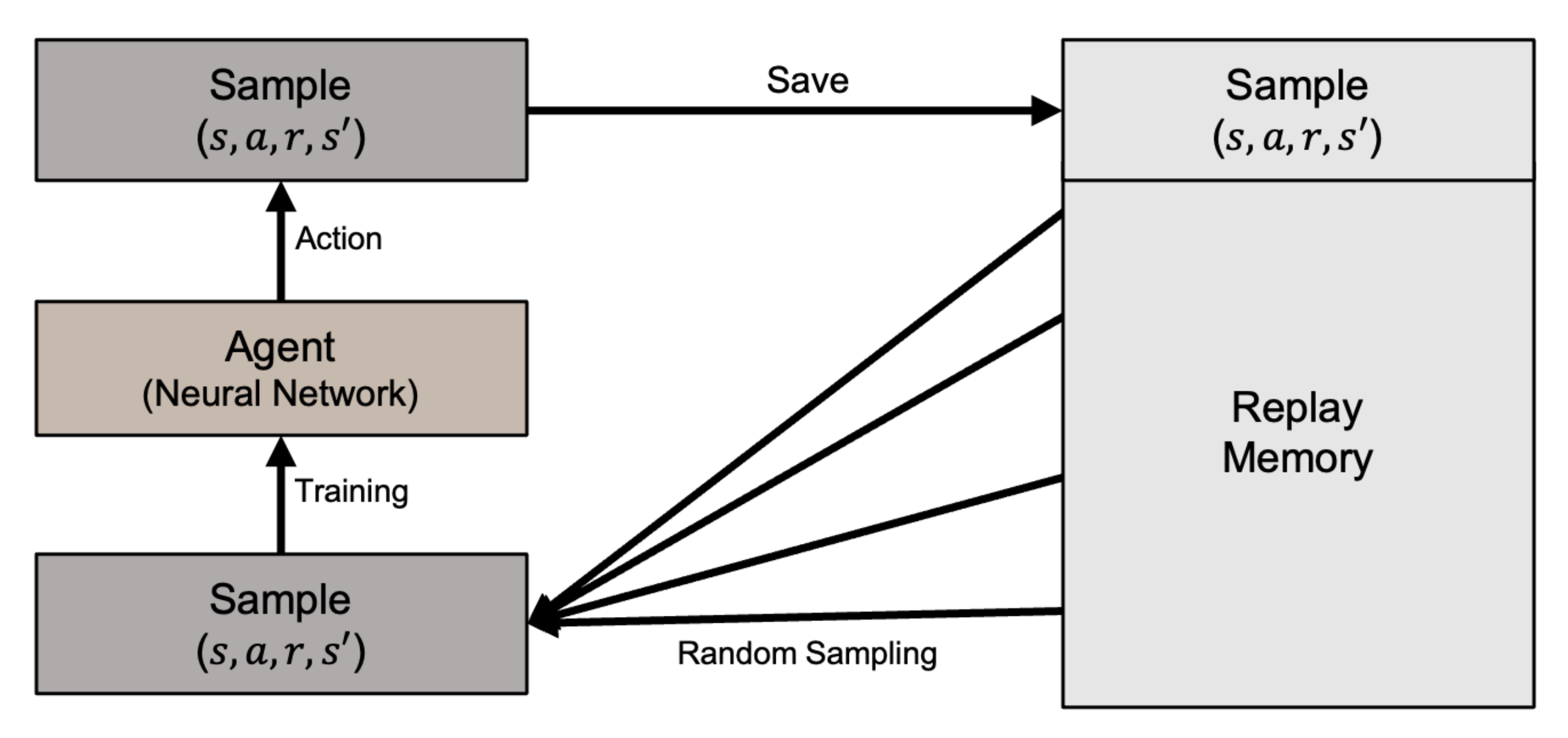
With Q-learning, the state–action combinations are stored in a table [35]. However, the Q-learning table cannot store the increasing number of continuous state variable values generated by our problem. Instead, we use the Deep Q-Learning method (DQN) with a deep neural network to approximate the Q function [24,29]. To resolve the issue of instability when a neural network attempts to approximate a non-linear function, DQN uses experience replay to randomly sample past actions instead of the most recent actions to proceed. DQN with the experience replay prevents the reinforcement learning from becoming excessively divergent due to a small update to Q. The DQN architecture is illustrated in Figure 7.
The number of distributions to choose for each zone is . The total number of possible fleet distributions is when z is set to 25, which is too many for a single decision agent to handle. Therefore, we run an independent agent for each zone that follows DQN-based policy learning separately with no cooperation, as discussed in the multi-agent reinforcement learning method [28]. With this approach, each agent in each zone considers only actions. For actions, agents choose a destination zone to be assigned with a 10% greater fleet proportion. The agent leaves one action without proportion augmentation. As a result, the IQL methodology proceeds as shown in Algorithm 4.
| Algorithm 4: Dispatch in IQL |
 |
4.4. DDR (Distribution Difference Reward)
We extend IQL by reflecting the distribution of the future order placements across all zones to the DQN’s reward function, which was the method used for a single taxi dispatch problem discussed by Zhou et al. [3]. This method, namely DDR, attempts to bring the taxi distribution in the following state close to the distribution of the passenger orders. We measure the spatial distribution of the available taxis in the subsequent state and that of the passenger distributions. We compute the difference between the two spatial distributions as shown in Equation (8). Then, we apply the difference to the reward function, as shown in Equation (9), where is the ratio of orders in to the total orders, is the ratio of supplies in to the total supplies, and is sum of differences between the ratio of orders and ratio of supplies in each zone. Note that, in IQL, the reward was based solely on estimated profit and revenue. With DDR, we expect the taxis to stay busy as taxis are assigned to the destinations with high follow-up demands.
4.5. Z-CMM (Zone-Agnostic CMM)
The final approach (Z-CMM) is not bound by the factitious zones that dissect the serviced area. Therefore, Z-CMM does not compute the proportion of taxis to be dispatched for destination zones. Z-CMM bypasses the proportion determination phase and proceeds straight to matching every taxi with the passengers based on CMM, as discussed in Section 4.1. Among the four approaches we have devised so far, Z-CMM is the most straightforward approach. It breaks the norm of all the previous works discussed in Section 2 that depends on dividing the service area into arbitrary zones. Z-CMM estimates the demand of the drop-off location and does not look further into future states. Thus, it is expected to make more prompt decisions than M-Greedy. The effectiveness of Z-CMM in generating revenue and profit is presented in the following section.
The key features of the approaches devised in this paper are summarized in Table 2.
5. Evaluation
We ran our taxi dispatch decision algorithms on an NVIDIA DGX-1 with an 80-Core (160 threads) CPU, 8 Tesla V100 GPUs with 32 GB of exclusive memory, and 512 GB of RAM. NVIDIA DGX-1 was operated with the Ubuntu 16.04.5 LTS server, and the machine learning tasks were executed through Docker containers. The machine learning algorithms were implemented with Python (v3.6.9), Tensorflow (v1.15.0), and Keras (v2.3.1) libraries.
For IQL and DDR, we used ReLU and linear kinds of activation function [36,37] and the Adam optimization function [38,39]. The learning rate was empirically set to 0.001, the discount factor was 0.99, and epsilon decay was 0.9999. Furthermore, each agent had one hidden layer with 256 perceptrons and a softmax layer for the output layer. In addition, we used the Mean Square Error (MSE) for the loss function. We published our source code on GitHub (https://github.com/YoungRaeKimm/Taxi-Dispatch accessed on 2 October 2021).
Our experiments are based on actual Seoul taxi operation data made publicly available by Seoul Metropolitan Government Big Data Campus (https://bigdata.seoul.go.kr/ accessed on 2 October 2021). The preprocessed datas are presented in query. The road network consists of 150-m links, and pick-up and drop-off coordinates and OD information are given. We used the data set collected over 24 h. We broke down the data into 30-s time steps, thus having 2880 time steps in total. In the case of models that require an episode for learning, such as IQL and DDR, one episode is 24 h. In addition, IQL and DDR learned while conducting a total of 50 episodes. There are 383,264 passenger calls in total, and the number of taxis to start with is fixed to 13,038. Demand and supply fluctuated over time in reality. The samples of the pre-processed taxi operation data are shown in Table 3 and Table 4.
We divided the service area into 2, 4, 8, and 25 administrative divisions for the zone-sensitive approaches.
We measured the performance of our approaches in terms of cumulative revenue and profit and the time taken to make a decision at every simulation episode.
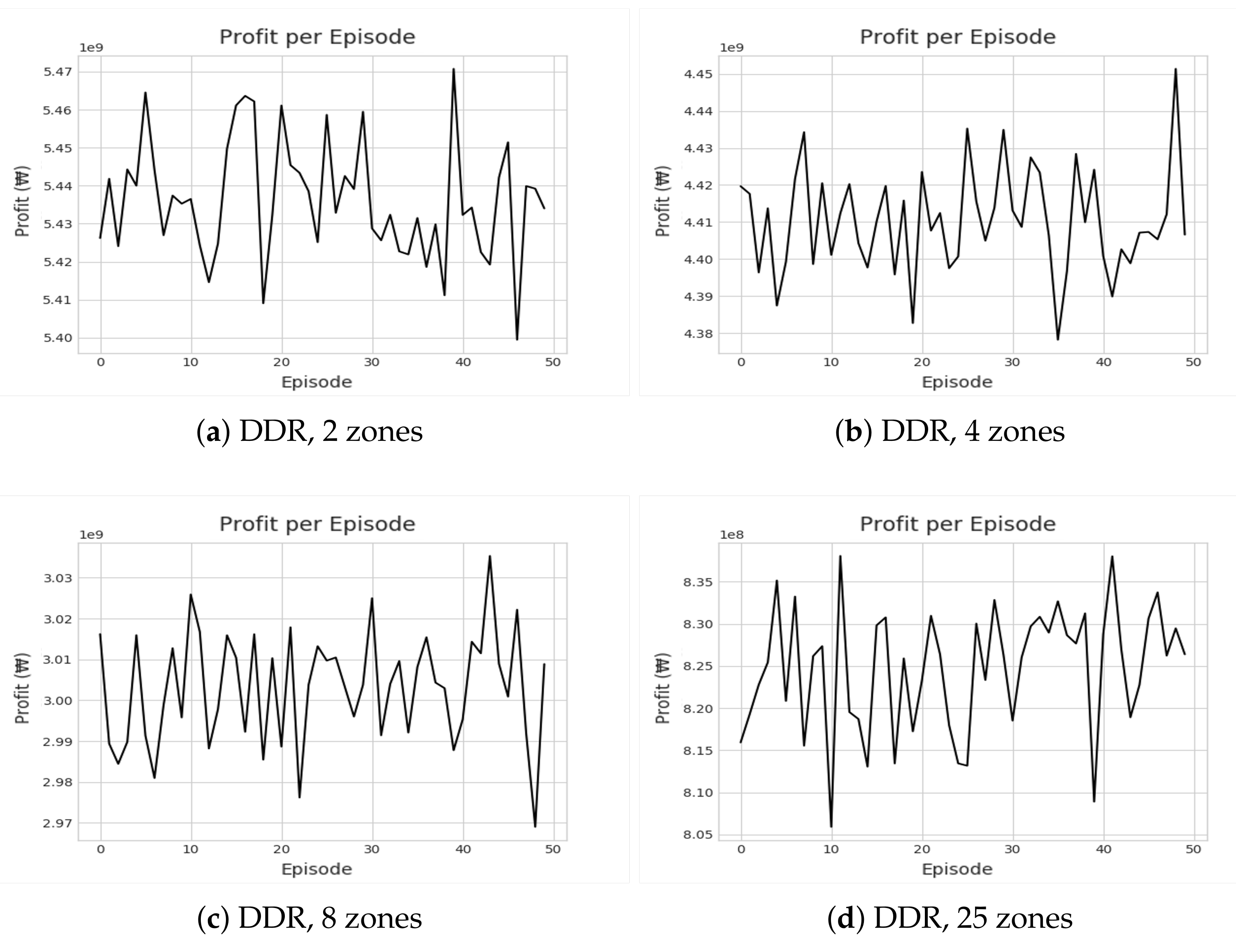
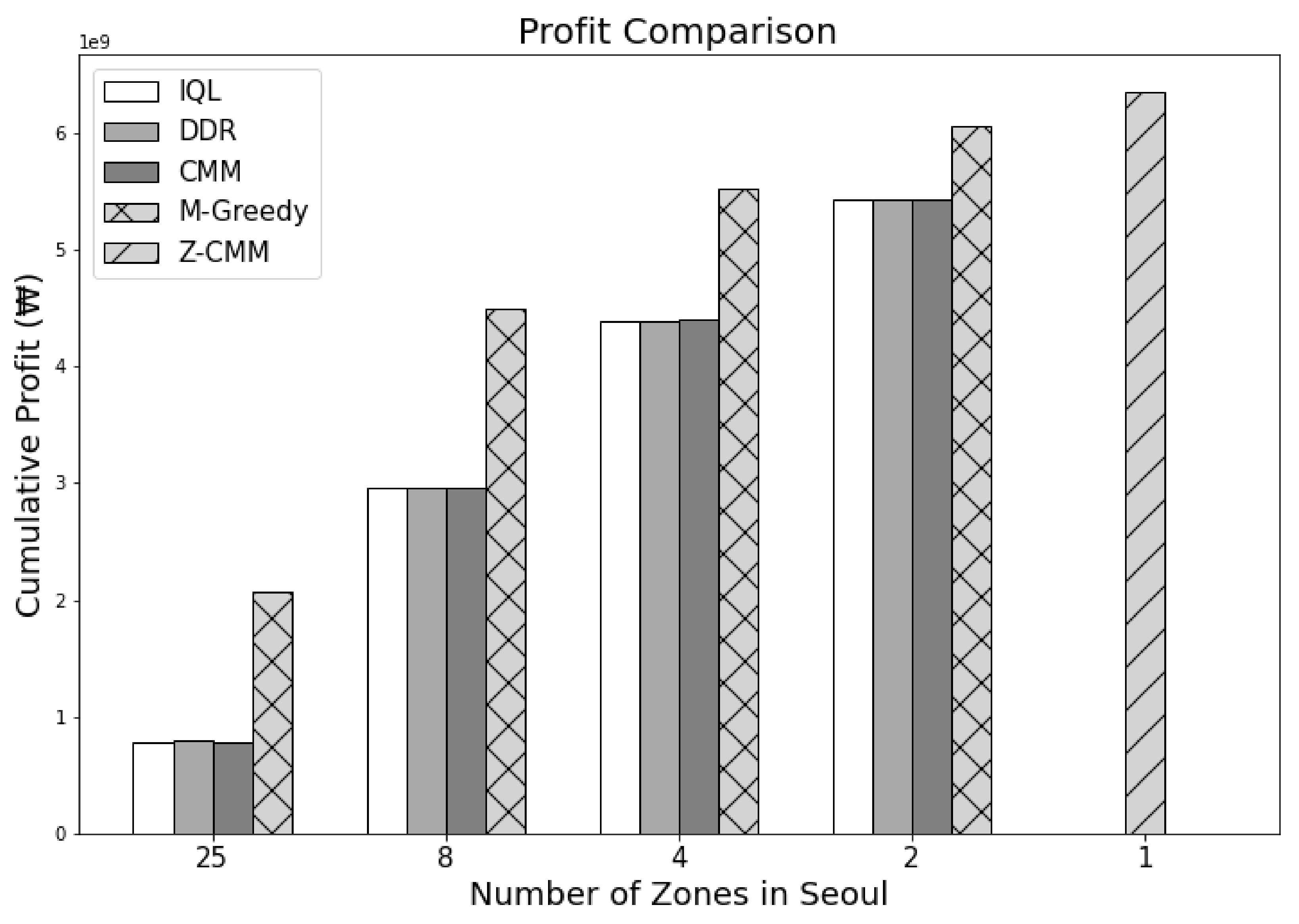
Figure 8 and Figure 9 show the cumulative profit during the reinforcement learning (RL) through IQL and DDR. Despite multiple iterations of reinforcement learning, we can see that the profit is highly divergent. In other words, no apparent profitable policy could be learned. Even accounting for the future states, approaches based on reinforcement learning could not outperform greedy approaches in terms of revenue and profit as shown in Figure 10 and Figure 11. Most interestingly, Z-CMM, which is not restricted by the service area divisions, yielded the highest revenue and profit compared to other approaches. Z-CMM generated 4.647 % and 4.982 % higher revenue and profit on average (equivalent to 0.3 billion Korean won and 0.28 billion Korean won more in revenue and profit), respectively, than the best zone-sensitive approach in the two-zone setting.
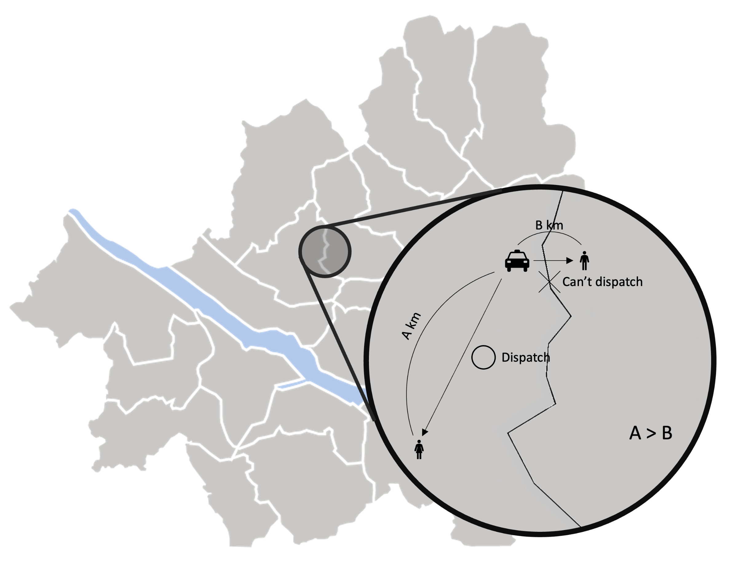
As we reduce the number of zones, revenue and profit increase for all zone-sensitive approaches. All zone-sensitive approaches restrict the taxis to be matched with a passenger within their predefined zone, even though matching the taxi to the much closer passenger call across the zone border can be more profitable, as illustrated in Figure 12. From this observation, we can safely conclude that the arbitrary division of the service area can be considered harmful. With Z-CMM being the top performer, a complicated computation to determine the fleet proportion among different zones is futile. A simplistic taxi passenger matching with CMM suffices.
The relatively poor performance of IQL and DDR resonates with the critical flaw many previous RL-based methods also have for the taxi dispatch decision problem. Note that assigning the taxi to a particular passenger is not at all the cause of a new demand for the drop-off zone in the subsequent time steps. In other words, a new demand after a drop-off occurs independently of the taxi assignment decided in the previous time step. However, given the deterministic MDP, RL is forced to learn the correlation between the two unrelated values—the demand in the future state and the taxi deployment decision in the previous state. The incorrect correlation attempt explains the high divergence seen in Figure 8 and Figure 9. Greedy algorithms avoid such false correlations. We attempted to address the stochastic nature by guiding DDR to yield a policy that moves the fleet to the zones with a probable high follow-up demand. However, this did not lead to any improvement, and DDR was on par with the basic CMM, which also accounts for the out-degree of the destination zones ( in Table 1). We were able to discover this problem as we used real demand distribution data, unlike the previous RL-based works that assume predetermined and fixed demands at every time step.
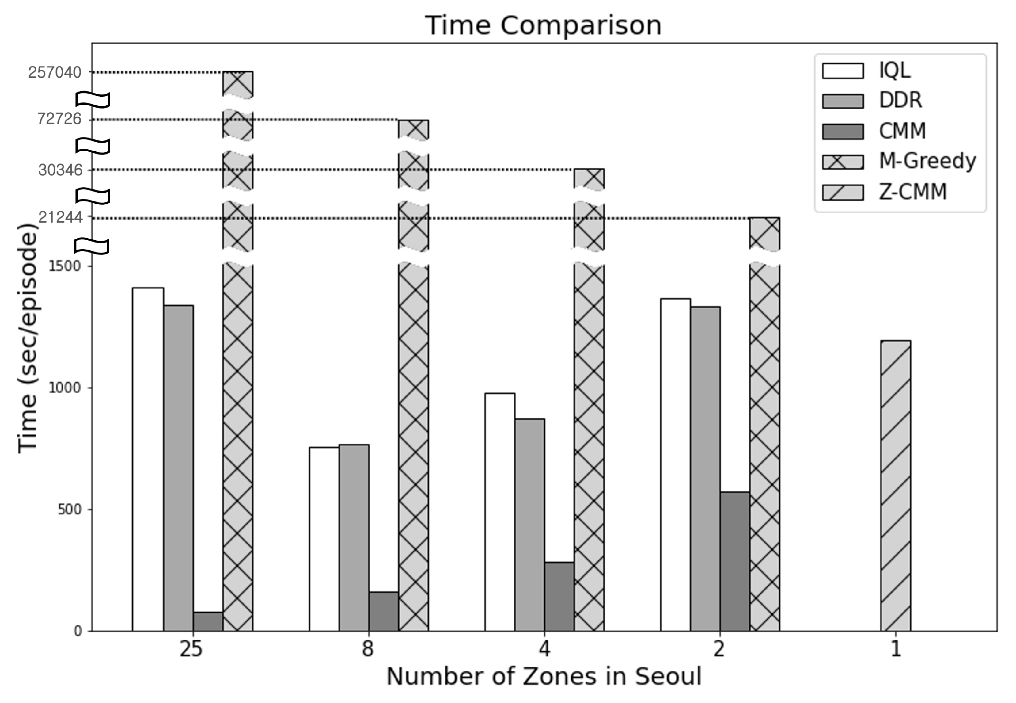
In terms of the time taken to determine the dispatch actions (Figure 13), CMM performed the best. On the other hand, M-Greedy consumed the most time—as much as 275,040 s per episode—when the number of zones was set to 25. M-Greedy mimics the farsightedness of the RL-based approaches by looking ahead to D future states. M-Greedy significantly outperforms the RL-based approaches. Compared to a basic zone-sensitive CMM algorithm, calculating the value of an action with the future states also considered was beneficial. Nevertheless, Z-CMM, with the simple removal of service area divisions, outperformed M-Greedy even without the future state considerations. The look-ahead mechanism can be introduced to Z-CMM as well. However, M-Greedy failed to finish the process of computing the top-k actions over D future states within the 30 s decision cycle. Hence, applying the excessively time-consuming look-ahead process to Z-CMM is not a viable option, as the number of cases to consider before computing the top-k cases is much higher. Even though CMM took the least time, Z-CMM remains our final recommendation as it makes full decisions safely within the time-bound and generates much higher revenue and profit.
6. Conclusions
One of the keys to the competitive edge of our approach is being agnostic of geographical zones when matching taxis and passenger calls. Contrary to the conventional methods in the past, we do not force the taxis to be matched only with the passengers within the same predefined zone when closer passengers are present in the neighboring zones. Our greedy algorithm based on passenger-to-driver and origin-to-destination distances and a straightforward estimation of the demand at the drop-off location ran quickly without the considerable training overhead that can be incurred by machine learning methods such as reinforcement learning (RL). Our evaluation using the actual taxi operation data from the Seoul metropolitan area reveals that our approach was 16.914% more profitable and generated 16.893% higher revenue on average than the state-of-the-art RL-based methods under any service dissection settings. Furthermore, the dissection of the service area into multiple zones and the determination of the fleet distribution among destination zones turned out to be less effective. Based on these findings, we can naturally conclude that our zone-agnostic greedy algorithm is suitable for taxi fleet management companies operating in large-scale cities, which require prompt and profitable dispatch decision-making. However, our study does not assess or take into account the satisfaction of passengers, which could be a critical factor to consider in future work. In addition, we plan to apply our methods to other metropolitan cities and evaluate the effect with the same empirical evaluation approach.
Author Contributions
Conceptualization, Y.Y.; methodology, Y.K., Y.Y.; software, Y.K.; validation, Y.K., Y.Y; formal analysis, Y.K., Y.Y.; investigation, Y.K.; resources, Y.K.; data curation, Y.K.; writing—original draft preparation, Y.K.; writing—review and editing, Y.Y.; visualization, Y.K.; supervision, Y.Y.; project administration, Y.Y.; funding acquisition, Y.Y. All authors have read and agreed to the published version of the manuscript.
Funding
This research was supported by the Korean Agency for Infrastructure Technology Advancement (KAIA) grant funded by the Ministry of Land, Infrastructure, and Transport (Grant 20TLRP-B148970-04), by the Basic Science Research Programs through the National Research Foundation of Korea (NRF) funded by the Korea government (MSIT) (2020R1F1A104826411), by the Ministry of Trade, Industry and Energy (MOTIE) and the Korea Institute for Advancement of Technology (KIAT), under Grants P0014268 Smart HVAC demonstration support, and by the 2021 Hongik University Research Fund.
Data Availability Statement
Data is available at https://bigdata.seoul.go.kr/.
Conflicts of Interest
The authors declare no conflict of interest.The funders had no role in the design of the study; in the collection, analyses, or interpretation of data; in the writing of the manuscript; nor in the decision to publish the results.
References
- Sutton, R.S.; Barto, A.G. Reinforcement Learning: An Introduction; MIT Press: Cambridge, MA, USA, 2018. [Google Scholar]
- Lin, K.; Zhao, R.; Xu, Z.; Zhou, J. Efficient large-scale fleet management via multi-agent deep reinforcement learning. In Proceedings of the 24th ACM SIGKDD International Conference on Knowledge Discovery & Data Mining, London, UK, 19–23 August 2018; pp. 1774–1783. [Google Scholar]
- Zhou, M.; Jin, J.; Zhang, W.; Qin, Z.; Jiao, Y.; Wang, C.; Wu, G.; Yu, Y.; Ye, J. Multi-agent reinforcement learning for order-dispatching via order-vehicle distribution matching. In Proceedings of the 28th ACM International Conference on Information and Knowledge Management, Beijing, China, 3–7 November 2019; pp. 2645–2653. [Google Scholar]
- Liu, Z.; Li, J.; Wu, K. Context-Aware Taxi Dispatching at City-Scale Using Deep Reinforcement Learning. IEEE Trans. Intell. Transp. Syst. 2020. [Google Scholar] [CrossRef]
- Park, J.H.; Lee, C.J.; Yoon, Y. Dynamic Pricing Based on Reinforcement Learning Reflecting the Relationship between Driver and Passenger Using Matching Matrix. J. Korea Inst. Intell. Transp. Syst. 2020, 19, 118–133. [Google Scholar] [CrossRef]
- Zhang, R.; Pavone, M. Control of robotic mobility-on-demand systems: A queueing-theoretical perspective. Int. J. Robot. Res. 2016, 35, 186–203. [Google Scholar] [CrossRef]
- Seow, K.T.; Dang, N.H.; Lee, D.H. A collaborative multiagent taxi-dispatch system. IEEE Trans. Autom. Sci. Eng. 2009, 7, 607–616. [Google Scholar] [CrossRef]
- Liao, Z. Real-time taxi dispatching using global positioning systems. Commun. ACM 2003, 46, 81–83. [Google Scholar] [CrossRef]
- Lee, D.H.; Wang, H.; Cheu, R.L.; Teo, S.H. Taxi dispatch system based on current demands and real-time traffic conditions. Transp. Res. Rec. 2004, 1882, 193–200. [Google Scholar] [CrossRef] [Green Version]
- Chung, L.C. GPS Taxi Dispatch System Based on A* Shortest Path Algorithm; Malausia University of Science and Technology: Kuala Lumpur, Malaysia, 2005. [Google Scholar]
- Liu, Z.; Li, Z.; Wu, K.; Li, M. Urban traffic prediction from mobility data using deep learning. IEEE Netw. 2018, 32, 40–46. [Google Scholar] [CrossRef]
- Qu, M.; Zhu, H.; Liu, J.; Liu, G.; Xiong, H. A cost-effective recommender system for taxi drivers. In Proceedings of the 20th ACM SIGKDD International Conference on Knowledge Discovery and Data Mining, New York, NY, USA, 24–27 August 2014; pp. 45–54. [Google Scholar]
- Yuan, N.J.; Zheng, Y.; Zhang, L.; Xie, X. T-finder: A recommender system for finding passengers and vacant taxis. IEEE Trans. Knowl. Data Eng. 2012, 25, 2390–2403. [Google Scholar] [CrossRef]
- Xu, J.; Rahmatizadeh, R.; Bölöni, L.; Turgut, D. Real-time prediction of taxi demand using recurrent neural networks. IEEE Trans. Intell. Transp. Syst. 2017, 19, 2572–2581. [Google Scholar] [CrossRef]
- Yang, H.; Wong, S.C.; Wong, K.I. Demand–supply equilibrium of taxi services in a network under competition and regulation. Transp. Res. Part B Methodol. 2002, 36, 799–819. [Google Scholar] [CrossRef]
- Chadwick, S.C.; Baron, C. Context-Aware Distributive Taxi Cab Dispatching. U.S. Patent App. 14/125,549, 19 March 2015. [Google Scholar]
- Myr, D. Automatic Optimal Taxicab Mobile Location Based Dispatching System. U.S. Patent 8,442,848, 14 May 2013. [Google Scholar]
- Papadimitriou, C.H.; Steiglitz, K. Combinatorial Optimization: Algorithms and Complexity; Courier Corporation: New York, NY, USA, 1998. [Google Scholar]
- Zhang, L.; Hu, T.; Min, Y.; Wu, G.; Zhang, J.; Feng, P.; Gong, P.; Ye, J. A taxi order dispatch model based on combinatorial optimization. In Proceedings of the 23rd ACM SIGKDD International Conference on Knowledge Discovery and Data Mining, Halifax, NS, USA, 13–17 August 2017; pp. 2151–2159. [Google Scholar]
- Zheng, L.; Chen, L.; Ye, J. Order dispatch in price-aware ridesharing. Proc. VLDB Endow. 2018, 11, 853–865. [Google Scholar] [CrossRef] [Green Version]
- Zhao, Y.; Xia, J.; Liu, G.; Su, H.; Lian, D.; Shang, S.; Zheng, K. Preference-aware task assignment in spatial crowdsourcing. In Proceedings of the AAAI Conference on Artificial Intelligence, Honolulu, HI, USA, 27 January–1 February 2019; Volume 33, pp. 2629–2636. [Google Scholar]
- Oda, T.; Joe-Wong, C. MOVI: A model-free approach to dynamic fleet management. In Proceedings of the IEEE INFOCOM 2018-IEEE Conference on Computer Communications, Honolulu, HI, USA, 15–19 April 2018; pp. 2708–2716. [Google Scholar]
- He, S.; Shin, K.G. Spatio-temporal capsule-based reinforcement learning for mobility-on-demand network coordination. In Proceedings of the World Wide Web Conference, San Francisco, CA, USA, 13–17 May 2019; pp. 2806–2813. [Google Scholar]
- Mnih, V.; Kavukcuoglu, K.; Silver, D.; Graves, A.; Antonoglou, I.; Wierstra, D.; Riedmiller, M. Playing atari with deep reinforcement learning. arXiv 2013, arXiv:1312.5602. [Google Scholar]
- Li, M.; Qin, Z.; Jiao, Y.; Yang, Y.; Wang, J.; Wang, C.; Wu, G.; Ye, J. Efficient ridesharing order dispatching with mean field multi-agent reinforcement learning. In Proceedings of the World Wide Web Conference, San Francisco, CA, USA, 13–17 May 2019; pp. 983–994. [Google Scholar]
- De Lima, O.; Shah, H.; Chu, T.S.; Fogelson, B. Efficient Ridesharing Dispatch Using Multi-Agent Reinforcement Learning. arXiv 2020, arXiv:2006.10897. [Google Scholar]
- Xu, Z.; Li, Z.; Guan, Q.; Zhang, D.; Li, Q.; Nan, J.; Liu, C.; Bian, W.; Ye, J. Large-scale order dispatch in on-demand ride-hailing platforms: A learning and planning approach. In Proceedings of the 24th ACM SIGKDD International Conference on Knowledge Discovery & Data Mining, London, UK, 19–23 August 2018; pp. 905–913. [Google Scholar]
- Tan, M. Multi-agent reinforcement learning: Independent vs. cooperative agents. In Proceedings of the Tenth International Conference on Machine Learning, Amherst, MA, USA, 27–29 July 1993; pp. 330–337. [Google Scholar]
- Tampuu, A.; Matiisen, T.; Kodelja, D.; Kuzovkin, I.; Korjus, K.; Aru, J.; Aru, J.; Vicente, R. Multiagent cooperation and competition with deep reinforcement learning. PLoS ONE 2017, 12, e0172395. [Google Scholar] [CrossRef] [PubMed]
- Kim, B.; Kim, J.; Huh, S.; You, S.; Yang, I. Multi-objective predictive taxi dispatch via network flow optimization. IEEE Access 2020, 8, 21437–21452. [Google Scholar] [CrossRef]
- Hartigan, J.A.; Wong, M.A. Algorithm AS 136: A k-means clustering algorithm. J. R. Stat. Soc. Ser. C (Appl. Stat.) 1979, 28, 100–108. [Google Scholar] [CrossRef]
- Ester, M.; Kriegel, H.P.; Sander, J.; Xu, X. A density-based algorithm for discovering clusters in large spatial databases with noise. In Proceedings of the Knowledge Discovery and Data Mining, Portland, OR, USA, 2–4 August 1996; Volume 96, pp. 226–231. [Google Scholar]
- Campello, R.J.; Moulavi, D.; Sander, J. Density-based clustering based on hierarchical density estimates. In Proceedings of the Pacific-Asia Conference on Knowledge Discovery and Data Mining, Gold Coast, Australia, 14–17 April 2013; Springer: Berlin/Heidelberg, Germany, 2013; pp. 160–172. [Google Scholar]
- Kirk, D.E. Optimal Control Theory: An Introduction; Courier Corporation: New York, NY, USA, 2004. [Google Scholar]
- Watkins, C.J.; Dayan, P. Q-learning. Mach. Learn. 1992, 8, 279–292. [Google Scholar] [CrossRef]
- Nair, V.; Hinton, G.E. Rectified linear units improve restricted boltzmann machines. In Proceedings of the International Conference on Machine Learning, Haifa, Israel, 21–24 June 2010. [Google Scholar]
- Glorot, X.; Bordes, A.; Bengio, Y. Deep sparse rectifier neural networks. In Proceedings of the Fourteenth International Conference on Artificial Intelligence and Statistics, JMLR Workshop and Conference Proceedings, Ft. Lauderdale, FL, USA, 11–13 April 2011; pp. 315–323. [Google Scholar]
- Kingma, D.P.; Ba, J. Adam: A method for stochastic optimization. arXiv 2014, arXiv:1412.6980. [Google Scholar]
- Ruder, S. An overview of gradient descent optimization algorithms. arXiv 2016, arXiv:1609.04747. [Google Scholar]
Figure 1.
Taxi dispatch decision process.

Figure 2.
Consider an example where 100 passenger orders exceed the supply of 60 taxis in zone B. We can assign more taxis to the zone with the highest expected revenue and profit-generation opportunities (for example, zone C). Such an approach would generate a better result than the naīve approach of dividing the fleets in proportion to the current demand for different zones without predicting the situation at the drop-off zones.

Figure 3.
Illustration of demand during (a) 30 s (12:00:00 to 12:00:30 a.m.), (b) 10 min (12:00 to 12:10 a.m.), and (c) during 24 h (12:00 a.m. to 12:00 a.m. the next day).
Figure 3.
Illustration of demand during (a) 30 s (12:00:00 to 12:00:30 a.m.), (b) 10 min (12:00 to 12:10 a.m.), and (c) during 24 h (12:00 a.m. to 12:00 a.m. the next day).

Figure 4.
Seoul is divided into (a) 2, (b) 4, (c) 8, and (d) 25 zones. The matching process occurs independently within each zone.
Figure 4.
Seoul is divided into (a) 2, (b) 4, (c) 8, and (d) 25 zones. The matching process occurs independently within each zone.

Figure 5.
Illustration of CMM after a single taxi-order pair is matched.

Figure 6.
In every look-ahead state, M-Greedy chooses the top-k distributions that yield the highest revenue and profit. In this figure, each block represents a top-k case after simulating all cases in the preceding state. Then, the platform looks ahead D time steps in the future. As a result, M-Greedy chooses the best case among cases once the computation is finished on the last look-ahead state. In this paper, we set k to 3 and D to 3.

Figure 7.
Illustration of DQN architecture.

Figure 8.
Illustrations of recorded cumulative profits by IQL under different zone settings.

Figure 9.
Illustrations of recorded cumulative profits by DDR for different zone settings.

Figure 10.
Comparison of the cumulative profit by each methodology during 24 h. The Z-CMM methodology recorded the highest profit.
Figure 10.
Comparison of the cumulative profit by each methodology during 24 h. The Z-CMM methodology recorded the highest profit.

Figure 11.
Comparison of the cumulative revenue by each methodology during 24 h. The Z-CMM methodology recorded the highest revenue among the methodologies.
Figure 11.
Comparison of the cumulative revenue by each methodology during 24 h. The Z-CMM methodology recorded the highest revenue among the methodologies.

Figure 12.
Zone-sensitive approaches did not allow the taxis to pick up a passenger in another service zone even though they are nearer than any other passengers within its zone. This is because the zone-sensitive approaches must determine the fleet proportions to different destination zones prior to matching taxis and passengers individually.

Figure 13.
Illustrations of time consumption by each methodology.


Table 1.
Definition of the key notations used in this paper.
| Notation | Definition |
|---|---|
| e | Episode time |
| Maximum episode time | |
| t | Simulation time step |
| Maximum simulation time steps | |
| The number of zones in Seoul | |
| The number of idle taxis | |
| d | The number of time steps simulated |
| D | The number of time steps to simulate |
| k | Top-k cases to be chosen in a single simulation time |
| Fleet state at time step t | |
| Fleet state at t in nth best simulation case | |
| Zone identified with i | |
| Vector of the orders’ distance from origin zone to destination zone | |
| The sum of OD distance of matched orders | |
| Matrix of the distance from orders to idle taxis | |
| Normalized PD | |
| Sum of PD distance of matched orders | |
| Out degree of the | |
| Ratio of orders in to the total orders | |
| Ratio of supplies in to the total supplies | |
| A distribution with jth highest profit chosen by agent of | |
| Sum of differences ratio of orders and ratio of supplies in each zone | |
| Calculated profit in a time step | |
| Calculated revenue in a time step | |
| Calculated reward in a time step |
Table 2.
Five methods for taxi dispatch decision making.
| Methods | Zone-Based Matching | Ratio of Taxis between Destination Zones | Myopic | Far Sighted | Taxi–Passenger Spatial Distribution |
|---|---|---|---|---|---|
| CMM | O | X | X | X | X |
| M-Greedy | O | O | O | X | X |
| IQL | O | O | X | O | X |
| DDR | O | O | X | O | O |
| Z-CMM | X | X | X | X | X |
Table 3.
Overview of order data.
| Pick Up Timestep | Pick Up Zone Number | Destination Zone Number | Pick Up Latitude | Pick Up Longitude | Drop Off Latitude | Drop Off Longitude |
|---|---|---|---|---|---|---|
| 0 | Zone 1 | Zone 1 | 37.616380 | 127.12491 | 37.4931945 | 127.029665 |
| 0 | Zone 1 | Zone 3 | 37.612991 | 126.92186 | 37.463410 | 126.527850 |
| … | … | … | … | … | … | … |
| 2879 | Zone 25 | Zone 25 | 37.493194 | 126.90832 | 37.6083009 | 127.034780 |
Table 4.
Overview of taxi data.
| Zone Number | Latitude | Longitude |
|---|---|---|
| Zone 1 | 37.40802 | 127.1442006 |
| Zone 1 | 37.795449 | 126.19642 |
| … | … | … |
| Zone 25 | 37.119776 | 126.048993 |
Publisher’s Note: MDPI stays neutral with regard to jurisdictional claims in published maps and institutional affiliations. |
© 2021 by the authors. Licensee MDPI, Basel, Switzerland. This article is an open access article distributed under the terms and conditions of the Creative Commons Attribution (CC BY) license (https://creativecommons.org/licenses/by/4.0/).
Share and Cite
MDPI and ACS Style
Kim, Y.; Yoon, Y. Zone-Agnostic Greedy Taxi Dispatch Algorithm Based on Contextual Matching Matrix for Efficient Maximization of Revenue and Profit. Electronics 2021, 10, 2653. https://0-doi-org.brum.beds.ac.uk/10.3390/electronics10212653
AMA Style
Kim Y, Yoon Y. Zone-Agnostic Greedy Taxi Dispatch Algorithm Based on Contextual Matching Matrix for Efficient Maximization of Revenue and Profit. Electronics. 2021; 10(21):2653. https://0-doi-org.brum.beds.ac.uk/10.3390/electronics10212653
Chicago/Turabian StyleKim, Youngrae, and Young Yoon. 2021. "Zone-Agnostic Greedy Taxi Dispatch Algorithm Based on Contextual Matching Matrix for Efficient Maximization of Revenue and Profit" Electronics 10, no. 21: 2653. https://0-doi-org.brum.beds.ac.uk/10.3390/electronics10212653
Note that from the first issue of 2016, this journal uses article numbers instead of page numbers. See further details here.