
Methods of Fast Analysis of DC–DC Converters—A Review


Department of Marine Electronics, Gdynia Maritime University, 81-225 Gdynia, Poland
*
Author to whom correspondence should be addressed.
Electronics 2021, 10(23), 2920; https://0-doi-org.brum.beds.ac.uk/10.3390/electronics10232920
Submission received: 26 October 2021
/
Revised: 22 November 2021
/
Accepted: 23 November 2021
/
Published: 25 November 2021
(This article belongs to the Special Issue Innovative Technologies in Power Converters)
Abstract
:The paper discusses the methods of fast analysis of DC–DC converters dedicated to computer programmes. Literature methods of such an analysis are presented, which enable determination of the characteristics of the considered converters in the steady state and in the transient states. The simplifications adopted at the stage of developing these methods are discussed, and their influence on the accuracy of computations is indicated. Particular attention is paid to the methods of fast analysis of DC–DC converters, taking into account thermal phenomena in semiconductor devices. The sample results of computations of the DC–DC boost type converter obtained with the use of the selected methods are presented. The scope of application of particular computation methods and their duration times are discussed. Computations were performed with the use of SPICE and PLECS.
Keywords:
power converters; electrothermal modelling; DC–DC converters; thermal phenomena; SPICE; PLECS; MOSFET; IGBT1. Introduction
DC–DC converters constitute an important group of impulse power electronic converters in which, depending on the topology, the constant input voltage is lowered or increased [1]. In these converters, there are semiconductor devices that play the role of fast switches and LC components that store energy and filter voltage and output current waveforms [2]. The essence of the operation of the considered class of circuits shows that their correct operation is possible only when the period of the signal controlling the transistors is much shorter than the time constants associated with the RLC components included in the DC–DC converter [3].
In the considered class of converters, apart from the electrical phenomena related to switching semiconductor devices as well as charging and discharging of LC components, thermal phenomena also occur in all converter components [4]. These phenomena are related to the nonidealities of the above-mentioned components, causing the occurrence of power losses in them. Thermal phenomena, e.g., self-heating, cause an increase in the internal temperature of electronic components, which also results in a change in the values of currents and voltages in the considered converters [5].
While designing power electronic converters, computer simulations play a key role [3,6,7]. Computer tools solving the systems of state equations describing the simulated system are commonly used for a circuit-level analyses of electronic circuits [3,8]. The most popular tools of this type include SPICE and SABER [3,8,9]. They contain physical models of semiconductor devices. Unfortunately, carrying out analyses of power converters in such programmes is time consuming, because their algorithms are not allowing quick solutions of the systems of stiff differential-algebraic equations [10].
Solving such systems of equations is a numerical problem. In the case of impulse systems, such as power electronic converters [11], it results from a significant difference between the period of transistor control signals, the duration time of transient states related to LC components contained in the converter, and thermal time constants characterizing thermal properties of the components of the analysed system [12].
There are also programs available on the market, such as PSIM and PLECS, which allow a significant reduction in the duration of computations [13]. In these programmes, switching of switches is described in a simplified manner. It is assumed in the computations that the switching times of the semiconductor elements are zero. Due to this approach, there is no time constant in the state equations, and only equations in two states of the transistor operation are formulated and solved—when it is turned on or off.
Figure 1 presents the classification of simulation methods for power electronic converters.
At the basic level, simulation methods for power electronic converters can be divided into isothermal and electrothermal methods. In isothermal methods, it is assumed that during the analysis, all components of the simulated system have the same temperature, equal to the ambient temperature. Such methods are implemented in SPICE-like circuit simulators. In the case of power electronic converters, due to the above-described problem of solving systems of stiff differential-algebraic equations, the analyses in such programmes are time consuming. The duration of calculations can be significantly shortened by using the averaged models method, in which only the average values of voltages and currents in the analysed circuit in the steady state are determined, which significantly simplifies the computed problem.
In electrothermal analyses, values of currents, voltages, and internal temperatures of the components of the circuit are simultaneously computed. Performing such analyses in circuit analysis programmes requires simultaneous solution of the equations describing electrical properties of the considered systems and circuit thermal models formulated with the use of the electric-thermal analogy. Typically, it has the form of an RC Foster or Cauer network [14,15].
Performing transient analysis of the power converter with the use of the thermal-electrical analogy in SPICE-like programmes for a circuit analysis is very time consuming [12]. That is why dedicated programmes to analyse transients were developed, such as PSIM and PLECS [13]. In these programmes, the duration time of transient analyses is much shorter because switching transistors and diodes in the circuit is modelled on the electrical level as ideal—with the duration of zero. This approach significantly simplifies computations. Even faster are electrothermal analyses of power electronic converters with the use of averaged models.
In all the above-mentioned methods, the internal temperature of the semiconductor device at a given moment in time is constant in the entire volume of the semiconductor structure. Meanwhile, in practice, there is nonuniform temperature distribution in the structure [16]. In order to model it correctly, it is necessary to use hybrid methods. In these methods, first time courses of the power emitted in the device are computed by means of a programme for analysis of electronic circuits. Based on these waveforms, a 2D or 3D thermal analysis is performed in a programme solving the heat conduction equation [17].
For many years, many research centres have been working on the development of new computational methods that allow for the performance of electrothermal analyses of power electronic systems in a relatively short time.
The aim of this paper is to review the so far published methods that allow for a reduction in the duration time of computer analyses of power electronic converters and comparing properties of these methods. Particular attention is paid to the methods of fast analysis of DC–DC converters with thermal phenomena in semiconductor devices taken into account. Such an aim is important, because these phenomena cause an increase in the internal temperature of semiconductor devices with an increase in power dissipated in them. A big increase in the value of such temperature can cause a strong reduction in the value of the lifetime of such devices and DC–DC converters with these devices. On the other hand, an increase in the device internal temperature causes a change in the courses of characteristics of the considered converters.
In the following sections of this article, the computational methods published so far and models implemented in popular simulation environments have been classified. Section 2 describes the methods of isothermal analysis of the DC–DC converters. Section 3 describes the problem of thermal phenomena in semiconductor devices. Section 4 describes selected methods of electrothermal analysis of power converters. Section 5 contains the results of computations carried out with the use of selected methods and the discussion of the obtained results.
2. Isothermal Methods
Analyses typically performed in programmes for a circuit-level analysis of electronic circuits are isothermal, which means that the internal temperature of all the analysed elements is constant during their operation and equal to the ambient temperature [7]. Computations performed by such a programme consist of solving differential-algebraic equations describing the analysed system. In the analyses of such systems, compact models are used, which especially for semiconductor devices have a complex form given in many papers, e.g., in [18,19,20].
The literature describes the methods of isothermal analysis of transients [7] and methods using DC or AC analysis with averaged models [6].
In Section 2.1, selected methods of isothermal transient analysis of power electronic converters are described, and in Section 2.2—the methods based on the use of averaged models and DC analysis.
2.1. Isothermal Transient Analyses
Isothermal transient analyses are the basic methods to analyse impulse systems in SPICE-like programmes. The greatest advantage of computational methods using transient analysis is the ability to precisely model parasitic capacitances and inductances of semiconductor devices. This allows for the correct mapping of the process of switching these elements as well as overvoltages and overcurrents related to this process.
In turn, the biggest disadvantages of these computation methods are:
- Long duration time of computations;
- A high level of models complexity embedded in SPICE-like programs;
- Problems with model parameter estimation.
The disadvantages indicated above are one of the main reasons why the literature offers numerous models of power semiconductor devices for isothermal analyses, whose authors report a higher accuracy than for the models built into peripheral analysis programmes. For example, in [21], an isothermal model of the IGBT was proposed, in [22]—the SiC BJT model, and in [23], an isothermal model of the SiC JFET transistor.
Unfortunately, the time needed to perform analyses using these models is longer than in the case of models built into SPICE. As shown in [24], the time needed to compute the output characteristic of the DC–DC boost converter using the model from [21] is as much as 14 days.
The method of modelling switching semiconductor devices is very important in transient analysis. In the simplest case, they are replaced by ideal switches. When using such a model, at switching times, infinitely high values of derivatives of terminal currents or voltages of the ideal switches occur, which can cause convergence problems or even computation interruptions. To counteract this problem, models of semiconductor devices in the form of a bivalent resistor are used.
Simple models provide analyses of properties of the circuit operation and accelerate simulation, but may contain discontinuities, e.g., time-varying circuit topologies must be considered. This requires the use of custom simulation methods. Much attention was paid to the problem of inconsistent initial conditions, and theoretical solutions can be found in [25,26].
The papers [27,28] propose an algorithm for transient analysis in DC–DC converters, with the PWM control using models of coils and capacitors associated with a memory-less convolution algorithm. The authors described the transistor using an inertia-less switch model with finite on and off resistance values, which protects the system against the occurrence of the Dirac pulses at the time of switching and omitting inertia and secondary phenomena. This method also ignores inertia in nonlinear components.
In the algorithm of transient analysis implemented in SPICE called further the ASP algorithm, in order to obtain the information about the values of voltages and currents in the circuit at the steady state, computations should be carried out in the time interval from the moment of switching on the tested circuit to the value equal to at least a few of the longest time constants of this circuit. In the considered converters, values of individual time constants related to the values of the used electronics components and the parameters of the control signal may differ from each other even by several orders of magnitude [12]. Therefore, from the point of view of computer analysis, these are the so-called rigid systems [10], in which the selection of the time step is determined by the value of the shortest time constant, and the analysis completion time necessary to obtain the steady state—the longest time constant. Hence, the determination of the value of the converter operating parameters in the steady state requires an analysis of transient states in the time interval corresponding to even many thousands of periods of the control signal, which is a time-consuming task [29].
In addition to the range of the analysis, understood as the time needed to obtain the steady state in the circuit, the duration time of computations is also influenced by the form of the component models used, because the models described by complex dependences require more mathematical operations in each iteration than the models described by simpler relationships. For this reason, the literature presents methods to analyse DC–DC converters, hereinafter referred to as fast methods, the purpose of which is to shorten the duration time of computations. These methods use simplified models of the components of this circuit, especially semiconductor devices. A typical simplification in the analysis of switching circuits, e.g., DC–DC converters, is modelling semiconductor devices with the use of ideal switches (used, e.g., in the papers [3,7,30,31,32,33]) or with the use of bivalent resistors (used, e.g., in the papers [28,34,35]). However, even with the use of such simple switching devices models and the ASP algorithm in SPICE, the computation time necessary to obtain the coordinates of one point on the steady-state characteristics is long.
The authors’ experience shows that the classic ASP algorithm, used in SPICE, with the physical models of semiconductor devices is time consuming in the case of the analysis of even nonisolated DC–DC converters. When using the ASP algorithm in SPICE, there is a limitation of the value of the minimum computation step [36], which is often the cause of computations interruptions by this programme in the case of the analysis of a circuit excited by a rapidly changing signal at a long range of the analysis [12]. In such a situation, an interval analysis should be performed by repeatedly running SPICE using the save bias and load bias commands and selecting experimentally the options values that determine the accuracy of computations, as well as the number of permissible iterations [12]. Often, the selection of the values of these options, ensuring the convergence of computations in the range of the assumed analysis time interval, is a difficult and time-consuming task.
Transient analysis of DC–DC converters requires the use of models of the components of these circuits in a form adapted to the requirements of the software used for computations, e.g., SPICE. This software includes, among others, models of semiconductor devices and passive components, which are described, among others, in the papers [37].
In SPICE, transient analysis is carried out with a variable calculation step, the value of which depends on the rate of changes in voltage in the nodes and currents in the branches and on the used range of the analysis [36,38]. In general, performing computations with a short time step makes it easier to achieve convergence. Therefore, the user can limit the maximum value of the computation step with the step ceiling parameter set when defining the transient analysis. When analysing the switched circuits controlled by a signal with a frequency from several dozen to several hundred kilohertz, the value of the step ceiling parameter should be selected in the range from single nanoseconds to several dozen nanoseconds. It is easier to obtain the convergence of calculations when this parameter is not an integer multiple of the natural power of 10, i.e., it is better to take the step ceiling value of 29.17 ns than 30 ns. Of course, from the point of view of limiting the duration time of computations and the size of the output file, it is preferable to choose the highest possible value of the mentioned parameter.
As mentioned above, one of the purposes of the analysis of DC–DC converters is to determine their characteristics at the steady state. The group of papers [39,40,41,42,43] concern the methods of accelerated computations until the steady state is obtained in DC–DC converters based on the results of transient analyses carried out within one period. These methods use piece-wise linear models of switches and require the use of special computer software that is not commercially available.
As stated in [44], the use of SPICE for the analysis of power electronic circuits causes a number of difficulties related to the use of complex, nonlinear models of semiconductor devices, problems with the convergence of computations, and long duration time of analyses.
The method to implement the accelerated steady-state analysis method in DC–DC converters, proposed in [42], consists of alternating computations with the use of the SPICE and the Mathematica software. According to this method, computations are performed iteratively, with SPICE carrying out a transient analysis for the time corresponding to one period of the control signal, while Mathematica, based on the obtained results of the computations, extrapolates the solution to the steady state. The main advantage of the considered method is a fast steady-state solution with nonlinear models of semiconductor devices, while the disadvantage is a big calculation error and the lack of access to the computation results at some nodes of the analysed circuit.
The method of fast calculation of the characteristics of the single-inductor DC–DC converters at the steady state presented in [45] is based on iterative transient analysis with the initial condition obtained from the averaged model. In the averaged model, the values of voltage drops on the diode and transistor terminals are obtained from the transient analysis. This method allows for the nonlinearity of semiconductor devices to be taken into account, and the duration time of computations is much shorter than when using the ASP algorithm, but at the same time, several times longer than the duration time of computations performed with the method described in the papers [34,46,47].
Properties of the methods of the isothermal transient analysis presented in this section are collected in Table 1.
2.2. Analysis Using Averaged Models
In the case of DC–DC converters, a significant reduction in the time needed to compute their DC characteristics is possible with the use of averaged models of the diode-transistor switch included in such a converter. By using averaged models and a DC analysis, the characteristics of the considered class of systems in the steady state can be determined. By performing a small-signal frequency analysis, the amplitude and phase characteristics of the analysed system can be determined. By means of the transient analysis, it is possible to determine the time courses of average values and currents in the system [3,38].
The first articles on the application of such models were based on the formulation of state equations and, then, transforming them into the form describing the average voltage and current values in the circuit [48,49]. The models presented in the cited papers concern the converter operation with the assumption of lossless components. In converters, especially low-voltage ones, these losses can significantly affect their characteristics [50].
The paper [51] presents the averaged model of the DC–DC converter taking into account losses in the LC elements, and in the paper [52]—a model taking into account losses both in the LC elements and those related to the conduction of semiconductor devices. In turn, paper [53] presents the use of the averaged DC–DC converter models in the design of a control system for such a converter. Paper [54] presents the results of the analyses carried out with the use of the averaged model of the 50 kVA DC–DC converter and experimentally demonstrated the correctness of the obtained computation results.
The classical approach to the formulation of average models of DC–DC converters is used, e.g., in the papers [55,56] to analyse the characteristics of the considered converters dedicated to the microgrid application at the steady state. In such analyses, isothermal piece-wise linear characteristics of semiconductor devices are assumed. Using these analyses, an influence of on-state resistance of the transistors and diodes on the characteristics of the considered networks was presented. Additionally, analyses of power losses were performed using the PLECS software.
A significant disadvantage of the above-described approach to formulating an averaged model is the necessity to formulate state equations for the converter, which, taking into account losses in semiconductor devices and LC elements, may have a very complex form. A solution to this problem was proposed in [53,57], where the model of a PWM switch (also called a diode-transistor switch in other papers) was described. The essence of this method is to replace in circuit-level simulations of switching devices a diode and a transistor with their equivalent averaged model. A similar solution was proposed in [58], along with the implementation of the model in the SPICE environment. The circuit form of such a model for a DC–DC boost converter with an IGBT transistor is presented in Figure 2 [24].
The values of currents I1 and I2 and voltages V1 and V2 in the circuit shown in Figure 2 are the average values of the diode and transistor currents and voltages, respectively. In turn, the control signal in this model is characterised by two parameters—frequency f and the duty cycle d. These parameters were used to describe the output voltages and currents of the controlled sources ET, ER, and GD. The controlled voltage source ET models the voltage drop depending on the converter output voltage and the duty cycle of the control signal. In turn, the controlled voltage source ET models the voltage drop on the turned on semiconductor devices; whereas, the controlled current source GD—the average diode current. The form of the equations describing the voltage or current output of these sources depends on the adopted description of the characteristics of semiconductor devices present in the switch under consideration. For example, assuming the piece-wise linear characteristics of these devices, we obtain the dependencies of the form [24].
where VD is the voltage on the conducting diode at zero current, RD—series resistance of the diode, VIGBT—collector–emitter voltage at the IGBT turned on at the zero collector current, and RIGBT—resistance characterising the slope of the output characteristic of the IGBT in the saturation range.
When ideal switches are used, VD, VIGBT, RIGBT, and RD are zero. On the other hand, for a PWM switch with a MOSFET, the VIGBT parameter is equal to zero, and the RIGBT parameter is equal to the drain-source on-state resistance RON.
Averaged models of DC–DC converters are especially useful for DC and small-signal analyses of these systems [59]. The paper [60] presents the averaged model of the DC–DC converter dedicated to such analyses, with particular emphasis on the losses related to the MOSFET switching. In turn, the paper [61] focused on the influence of properties of the coupled coils used in the converter on its frequency characteristics.
The paper [62] shows how to use the PWM switch model for the analysis of converters with galvanic isolation, and the paper [63] for the analysis of resonant converters. The application of the analysis method with the averaged model of the PWM switch enables a significant reduction in the duration time of computations in relation to the methods that use transient analysis [50].
Properties of the isothermal averaged models presented in this section are collected in Table 2.
3. Thermal Phenomena in Power Converters
In all the computation methods described in the previous section, it is assumed that the internal temperature of all the electronic components contained in the converters is equal to the ambient temperature. Meanwhile, due to thermal phenomena (self-heating and mutual thermal couplings), the temperature of all the converter components increases with an increase in power dissipated in them [64]. The closer they are to each other, the stronger the mutual thermal couplings between them. They cause an increase in the temperature of the components during their operation [65,66]. Thermal couplings occur not only between the components, but also inside them, e.g., in the case of power modules between semiconductor structures placed in the common case [67,68], and in the case of inductive components between the core and its windings [69,70].
Accurate determination of the temperature value of electronic components is of key importance for the proper estimation of their lifetime. Each 8 K internal temperature of a semiconductor device results in a twofold reduction in its lifetime expectancy [71]. Therefore, electrothermal simulations are of particular importance in the design of power converters. The result of these simulations are the values or waveforms of voltages and currents in the analysed converter and the internal temperature of its components. The results of these simulations allow for the selection of the cooling system, ensuring safe working conditions of the designed converter. The correct estimation of the internal temperature of semiconductor devices requires the correct determination of power losses in this device. The power lost at the steady state is easy to compute. In turn, the problem of determining losses in semiconductor devices taking into account oscillations (overvoltages and overcurrents) is described, among others, in the papers [72,73].
In order to carry out electrothermal analyses of the selected electronic circuit, special electrothermal models are necessary, which take into account mutual interactions of electrical and thermal phenomena occurring in the electronic components. The structure of such models is shown, among others, in [74]. In the considered class of models, there are blocks describing an increase in the internal temperature of the considered elements caused by thermal phenomena. Such models may take the form of 1D, 2D, or 3D microscopic models or compact models.
Microscopic thermal models make it possible to determine time–spatial distribution of the temperature of electronic components [75]. In contrast, compact thermal models make it possible to determine waveforms of one internal temperature, characterising the thermal state of each semiconductor device [76]. In the next section, a method of electrothermal analyses of DC–DC converters, using both the detailed and compact thermal models, will be considered.
4. Electrothermal Analyses
Due to the importance of thermal properties for the design of power electronic converters, electrothermal simulations of such systems are of particular interest [66,77]. However, taking into account thermal phenomena in conventional transient analyses carried out using SPICE-like programmes, as a result of the problem of solving a system of stiff differential-algebraic equations described in the Introduction, leads to an extension of computation duration time much more than the accepted time by engineers. Therefore, numerous methods of reducing this time have been proposed in the literature. Some of these methods are described below. Section 4.1 describes methods implementable in SPICE-like circuit simulators dedicated to transient analysis, Section 4.2—electrothermal analyses using averaged models, and Section 4.3—hybrid analysis methods that require combination of at least two simulation programmes.
4.1. Methods Based on Transient Analysis
The basic method to perform an electrothermal transient analysis is the implementation of the circuit diagram of the analysed system using isothermal models of the system components in the circuit analysis programme and coupling them with compact thermal models in the form of RC Cauer or Foster networks [53]. The general form of the focused electrothermal model of a semiconductor element is shown in Figure 3 [78,79,80].
The considered electrothermal model consists of three components: the electrical model of the form given by the function f(v,i), describing the relationship between voltages v and currents i of the modelled device; the power model of the form given by the function g(v,i), enabling the determination of power pth dissipated in the modelled device; the thermal model described by the function h(pth), in which the value of the internal temperature Tj occurring in the equations representing an electrical model is computed.
The form of electrothermal models of semiconductor devices has been described in numerous papers. In many papers, such models dedicated to the SPICE programme were presented. For example, the model of the SiC MOSFET power module is given in [65], a thermal model of electronics components is proposed in [79], a model of power MOSFET is described in [81], and a model of SiC power BJT is described in [82]. From the point of view of applications in the analysis of pulse systems, important are hybrid electrothermal models described, among others, in [83]. These models use a combination of isothermal models of semiconductor devices built into SPICE and the controlled voltage or current sources that model the influence of temperature on voltages or currents of these devices. The advantage of these models is good convergence of computations and a shorter duration time of computations in relation to electrothermal models containing only the controlled sources and passive components.
However, an electrothermal model formulated in this way with a linear thermal model is characterised by a relatively poor accuracy in computing the internal temperature of semiconductor devices. It results from the fact that thermal resistance of a semiconductor component is not constant, as it is assumed in linear thermal models based on the Foster and Cauer networks [84]. In the models described in [81,82], the value of thermal resistance depends on the power emitted in it, and in [67,85]—on the junction temperature of the semiconductor device and the ambient temperature.
A relatively simple method of shortening the time needed to perform computations to obtain the steady state is to artificially shorten the longest thermal RC time constant in a thermal model with the Cauer or Foster structure [86]. This method allows for a precise determination of the mean value of the junction temperature of semiconductor devices in the steady state, but due to the shortening of the longest thermal time constant, it requires a constant load value for the entire duration of computations. The scope of this method is limited to the analysis of the steady-state properties of the system.
A more complicated, but also more effective, method to reduce the duration time of computations is the use of dedicated computation algorithms to estimate the value of the internal temperature of semiconductor devices at the steady state. In [12], a memoryless convolutional algorithm is proposed, which allows for quickly obtaining voltage, current, and temperature waveforms inside the DC–DC converter components in the steady state. On the other hand, in [87], an algorithm to analyse the transient states of power converters based on the envelope-following method implemented in a dedicated simulation tool is proposed. Another algorithm for computing the steady-state voltage and current waveforms of DC–DC converters was proposed in [78].
The methods described in [12,78,87], despite their good accuracy, are not practical due to difficult [12] or impossible implementation in popular circuit-level simulation programmes. Such a problem does not occur in the case of the method described in [88]. In this method, the transistor is modelled as a lossy switch with a simplified gate circuit model. This approach makes it possible to obtain the result of the electrothermal analysis in PSCAD in the time close to the time needed for the analysis of the system, in which the transistors are replaced by ideal switches. The accuracy of the presented method is negatively affected by the use of a linear thermal model.
There are also programmes popular among engineers for electrothermal analysis of peripheral power converters, such as PLECS or PSIM. Electrical properties of transistors and diodes are modelled in them using the piece-wise linear function. In turn, to model their thermal properties, more complicated models of losses in transistors and diodes are used. They are based on the interpolation of the coordinates of points entered by the user, both from the datasheet DC characteristics and the dependence of energy losses in the transistor-switching process on selected factors [55,56]. Such a method of performing computations make it possible to obtain its relatively short duration time.
Unfortunately, the simplified description of the switching process of semiconductor devices makes it impossible to model overvoltages and overcurrents occurring in the modelled converter, which increase the value of energy losses in the switching process [72,73]. As a result, the value of the power dissipated in semiconductor devices determined in these programmes is always underestimated [76]. Linear thermal models implemented in these environments in the form of the Cauer or Foster network also negatively affect the accuracy of computations in these programmes. To improve it, the algorithm presented in [13] can be used, which allows for taking into account the dependence of thermal resistance on the junction temperature of the device.
4.2. Methods Using Averaged Models
As in the case of isothermal models, and also in the case of electrothermal analysis, averaged models allow for obtaining the result of computations in the shortest time. By mixing the above-described isothermal model of a diode-transistor switch with a linear compact thermal model, it is possible to obtain a converter model that models its electrothermal properties with good accuracy at low switching frequency values. Such models were formulated for the MOSFET [50,89] and the IGBT [90]. Of course, the output voltages or currents of the controlled sources included in the averaged models depend on the temperature inside the diode and the transistor, computed in the thermal model.
In order to accurately model thermal properties of transistors operating with a high switching frequency, it is necessary to take into account in the model the energy losses associated with its switching. A model of a switch with a SiC MOSFET formulated in such a way is presented in [91]. It also allows for predicting changes in the resistance of the switched-on channel of this transistor related to its aging and taking into account the influence of this phenomenon on the value of the internal temperature of this device.
In the case of the averaged electrothermal models described above, their authors focused on determining the internal temperature of the diode and the transistor contained in the converter. Meanwhile, from the point of view of designing DC–DC converters, the properties of inductors are of great importance. Losses occurring both in the core and in the winding of these components lead to an increase in their temperature, both due to the self-heating phenomenon and thermal interactions between them [92]. The averaged model enabling the computation of not only the internal temperature of the transistor and the diode, but also the temperature of the core and the winding of the inductor operating in the DC–DC converter is presented in [93].
Figure 4 shows a network representation of the electrothermal model of the PWM switch with a MOS transistor and a diode described in [92].
There are four blocks in this model: main circuit, CCM/DCM, aided block, and thermal model. The main circuit corresponds to the isothermal averaged model of the PWM switch shown in Figure 2a, with the description of the controlled sources ET, ER, and GD, where the internal temperatures of transistor TT or the diode TD computed in the thermal model occur.
The CCM/DCM block is used to set the operating mode of the analysed converter (CCM or DCM) and the value of the equivalent duty cycle of the control signal represented by the voltage at the voltage source Eu. This voltage depends, among others, on inductance of the inductor L in the analysed converter. In each of these modes, different relationships describe the sources included in the main circuit.
The controlled voltage sources occurring in the aided block describe the dependence of the parameters, describing a voltage drop on the enabled semiconductor devices on their junction temperature. The thermal model enables the determination of the junction temperature of the transistor and the diode in the steady state, taking into account the self-heating phenomenon. A detailed description of the considered model, along with the analytical dependences describing individual components of this model, is included in [92].
In order to use the presented model in practice, it should be included in the analysed converter in the place of the transistor and the diode as follows: Terminals 1 and 2 should replace the terminals of the drain and the source of the MOSFET. The signal of the duty cycle should connect the control signal to the corresponding terminal 5. Finally, terminals 3 and 4 should replace terminals of the diode.
In [94], the electrothermal averaged nonlinear models of DC–DC converters are proposed. These models take into account the influence of parameters of the transistor control signal and the duration time of the transistor and diode-switching process on the operating parameters of the considered converters and on power losses in the semiconductor devices. The disadvantage of these models is their low versatility—such a kind of model must be formulated for each converter system separately.
In the paper [95], a method taking into account the thermal inertia of semiconductor devices and mutual thermal couplings between these devices for the characteristics of DC–DC converters is proposed. In the cited paper, an averaged model of a PWM switch is used, and RC networks are used in the thermal model. It was shown that with the use of this model, it is possible to determine both the characteristics of the DC–DC converter in the steady state and the waveforms of the internal temperature of the MOSFET and the diode. It was also shown that the cooling conditions of semiconductor devices and mutual thermal couplings between them can cause significant changes in the converter output voltage and the internal temperature of these devices.
In the papers cited above, the computations were made assuming that power is lost in semiconductor devices only when they are turned on; whereas, power losses related to switching were neglected. This approach is justified only when the switching time of these devices is much shorter than the period of the control signal [96]. In the paper [97], the limitations of the averaged model of the PWM switch with the IGBT were analysed. The tests were carried out on the example of a boost converter operating at a wide range of frequencies, the duty cycle of the control signal, and load current. It was shown that when the considered converter operates in the CCM mode, the averaged model described above ensures a satisfactory accuracy of computations. On the other hand, in the DCM mode, at high frequency values and low load current values, the values of the internal temperature of semiconductor devices are lowered, and the output voltage of the converter is overestimated. The cause of these discrepancies is the problem of how to correctly determine the value of the duty cycle d, resulting from the comparability of the switching on and off time of semiconductor devices with the control signal period. This error can be reduced by taking into account the transistor on and off times when computing d factor.
It was also indicated that switching losses in the IGBT significantly affect the characteristics of the considered converter. Modifications of the description of power losses in this transistor were proposed, and it was shown that it improves the accuracy of calculations. The need to take into account the nonlinearity of the thermal model of semiconductor devices and the modification of the description of losses in the transistor at low load current values was also indicated.
4.3. Hybrid Methods
When formulating compact electrothermal models, it is assumed that the heat in the semiconductor device is pointedly dissipated, and its internal temperature is characterised by one value. Meanwhile, in the real semiconductor devices, there is nonuniform temperature distribution, and the heat is released only in a part of the device’s volume, e.g., for the MOSFET—in its channel. By solving thermodynamics equations in the dedicated simulation programmes, it is possible to determine the temperature distribution in the entire volume of the transistor. Unfortunately, such simulations are long lasting and require the detailed material, thermal, and geometric data on the structure of the modelled device. Moreover, programmes dedicated to such simulations are designed to perform computations of temperature distribution for one device and are not designed to perform peripheral analyses necessary for the design of power electronic circuits [98]. Therefore, the literature proposes methods that allow for combining the possibilities of circuit simulations in the field of designing electronic circuits and 3D thermal modelling of the devices contained therein [99].
To make such a combination possible, it is necessary to transfer to the 3D thermal model data on the waveforms of power dissipated in particular devices. The time–space temperature distributions are, then, determined, typically using the finite element method (FEM). The obtained temperature waveforms should be aggregated into the form of transient thermal impedance, and then, on its basis, the values of the parameters of the thermal model based on the Cauer or Foster network in the network simulator should be determined. A significant problem is the high order of the focused thermal model obtained from such a transformation [100]. The solution to this problem was proposed in [101], allowing for a significant reduction in the computation time for power transistors using the model order reduction method. This method was also used to analyse the operation of selected integrated circuits [102,103], multi-structure power transistors [98], and power modules [104].
A different approach to solving this problem was proposed in [105]. In the cited paper, three simulation software protocols were coupled: in SPICE voltage and current waveforms are determined using a compact electric transistor model. On their basis, the losses in the transistor related to its conduction as well as switching with the use of MATLAB are computed. The information about the lost power is transferred to Simulink, in which a compact thermal model based on the ANSYS Icepak software was implemented. On the basis of this model, the waveforms of the internal temperature Tj and the case temperature TC of the transistor are computed. This approach allows for obtaining simulation results in a relatively short time, while taking into account the influence of the temperature properties of the materials, from which the transistor and its heat sink are made. A similar approach was proposed in [75] for the analysis of circuits containing IGBT modules. Unfortunately, in the cited papers, the influence of the transistor internal temperature on the power losses in this device was omitted. This can lead to incorrect computation results.
In all the thermal models cited in this section, the finite element method (FEM) was used in the computations. The finite volume method (FVM) was used in [106], and the finite difference method in [17].
Hybrid methods have a special potential in assessing the reliability of power electronic converters. The paper [107] proposes the use of a hybrid electrothermal analysis method to model the thermal reliability of inverters used in electric vehicles.
In the cited paper, the information on the location of the heat source in the structure of the transistor was omitted. There was no information either as to whether this source was punctual or distributed. The heat source is always assigned to a specific layer—a cuboid-shaped volume (e.g., silicon) that is a part of the heat-flow path. However, the authors do not have any knowledge of a paper in which a thermal model of a transistor is described, which would enable to determine the space–time distribution of the internal temperature during its operation in a switched mode converter. This task is currently too complex for a numerical solution in an acceptable time.
The papers [76,108] propose a method to determine power losses in the transistors included in switched mode power converters and their internal temperature. This method uses the Fourier equations characterising the heat flow, and the calculations were made with the use of MATLAB. It was proved that the calculation time using this method is much shorter than the method using the detailed thermal model and FEM.
Properties of the methods of electrothermal analyses presented in this section are collected in Table 3.
5. Results of Computations
The presented methods of the analysis of DC–DC converters differ in the accuracy of the obtained computation results, the number of physical phenomena taken into account, and the duration time of the computations. Selected methods of the above-mentioned were experimentally verified, and the results of this verification were presented, inter alia, in many papers, e.g., [12,13,50,90,93]. In order to assess the usefulness of the selected methods, computer analyses were carried out to determine the DC characteristics and waveforms of voltages, currents, and internal temperatures of semiconductor devices for selected DC–DC converters operating at different values of supply voltage and load resistance.
The investigations were performed for a DC–DC boost converter. The diagram of this converter is presented in Figure 5.
In the considered network, the voltage source Vin represents the converter input voltage; whereas, R0 is load resistance. Voltage source Vctr generates the rectangular pulses train of values equal to zero in a low level and 15 V in a high level, frequency f, and duty cycle d. Values of the components of this converter are as follows: R1 = 100 Ω, C = 100 μF, and L = 100 μH. The following semiconductor devices are also used: the transistor IRF840 and the diode BY229.
In Figure 6, Figure 7, Figure 8 and Figure 9, the computed characteristics of the boost converter determined with the use of various calculation methods were compared. In these figures, particular computation results are marked as follows. The dashed lines refer to the results of isothermal analyses, and the solid lines—to the electrothermal analyses. The black lines are for transient analyses with ideal switches (curves ideal transient analysis), the brown lines—for transient analyses with nonlinear models of semiconductor devices (curves nonlinear transient analysis), the blue lines—averaged models with ideal switches (curves averaged ideal model), the green lines—averaged models with linear models of the PWM switch with the MOSFET (curves linear averaged model), and the red lines—the MOSFET transistor model in the PLECS programme, taking into account switching losses (curves PLECS). In the electrothermal analyses performed in SPICE, only one thermal time constant is taken into account.
Figure 6 and Figure 7 show the obtained dependences of the output voltage Vout of the considered converter on its load current Iout determined at the supply voltage Vin equal to 6 V (Figure 6) and 48 V (Figure 7), respectively. In turn, Figure 8 and Figure 9 show the dependences of the internal temperature of the transistor corresponding to the characteristics shown in Figure 6 and Figure 7. The computations were performed at the frequency f = 100 kHz and the duty cycle d = 0.5 of the control signal of the tested converter. The load of the converter is resistive, the inductance of the inductor is L = 100 μH, and the capacitance of the capacitor is C = 100 μF.
As can be seen, the courses of dependences Vout(Iout) obtained by most of the used computation methods are similar. Only the courses obtained using transient analysis with ideal switches do not have a proper shape in DCM mode. This is a result of omitting the switching time of semiconductor devices, which causes synchronous current conducting by both these devices during the switching process. For other of the used computation methods, the differences between obtained Vout(Iout) dependences are visible only at very low and very high values of Iout current. For high values of this current, an influence of voltage drops on the turned-on semiconductor devices is visible. In this range of converter operation, the differences between obtained values of Vout voltage are equal to even 60% at Vin = 6 V (Figure 6) and even 30% at Vin = 48V (Figure 7).
In Figure 6, it is visible that at the low Vin value, the voltage drop on the MOSFET is so high that the diode cannot switch off, and Vout is equal to the difference between the Vin voltage and the diode forward voltage. In this range of converter operation, the course Vout(Iout) is a horizontal line. This effect is not observed at a higher value of Vin voltage equal to 48 V (Figure 7). For very high values of Iout current, the values of Vout voltage are underestimated.
The dependences TT(Iout) are monotonically increasing functions, except for the course obtained using SPICE electrothermal transient analysis in the range of small values of Iout current (Figure 9). In this range, the big influence on this temperature has power losses in semiconductor devices during a switching process. Differences between values of TT temperature computed using all the considered methods are the biggest at high values of Iout current. In this range, the highest values of the MOSFET internal temperature are obtained for the averaged electrothermal model. They are higher even by 30 K than values of this temperature obtained using other considered electrothermal models.
Table 4 compares the duration time of the computations, the results of which are shown in Figure 6, Figure 7, Figure 8 and Figure 9.
As it can be seen, the computations performed with the use of averaged models are the fastest. Compared with the duration time of the transient analysis, the analyses performed with the use of the averaged models are even 25,000 times longer. It is also worth noting that the results of isothermal analyses are much shorter than the corresponding electrothermal analyses (up to 10 times). This is due to significant differences in the level of complication of the models used. The computations performed with PLECS are much longer than DC analyses performed with the use of averaged models and shorter than the isothermal and electrothermal analyses carried out in SPICE with the use of transient analysis.
With the use of the computation methods described above, an analysis of power losses in semiconductor devices can be performed. Of course, such an analysis is possible only in the case when such devices are not modelled using ideal switches. On the basis of the computed values of power losses in semiconductor devices, the energy efficiency of the considered DC–DC converters can be calculated. For example, an influence of selected factors on energy efficiency of selected DC–DC converters is considered in the papers [12,24,50,55,90,94].
All the considered computation methods make it possible to perform an AC analysis in SPICE. As a result of such analyses, one can obtain frequency characteristics describing the relations between AC components of voltages in the analysed DC–DC converters. Unfortunately, the analyses of harmonics of voltages and currents can be performed using the transient analysis, only. In such analysis, physical models of semiconductor devices should be used.
6. Conclusions
This paper presents selected methods of fast analysis of power converters. The basic problems related to the computer analysis of this class of converters are described, and selected methods enabling the reduction in the time necessary to obtain the computation results in the steady state are discussed. Both methods using transient analysis as well as DC analysis using the averaged models are indicated. The possibility of using models of semiconductor devices with different accuracy was indicated—from the models in the form of ideal switches to the physical electrothermal models. Using various simulation programmes is also considered.
There are two conflicting expectations in the computer analysis of electronic circuits. The duration time of computations should be short and the accuracy of these computations high. In turn, different accuracy of computations is required at different stages of the circuit design. Therefore, it is justified to use the models and computation methods characterised by different accuracy and time consumption. For example, to verify the concept of the system operation, fast methods characterised by moderate accuracy and the use of simplified models of electronic components are sufficient. Additionally, the influence of various factors on the accuracy of the computations depends on the power, load, and cooling conditions of the systems under consideration. Therefore, analytical methods of different accuracy and complexity are needed.
As shown in the previous section, the considered methods have different properties. Selected features of these methods are summarised in Table 5.
The shortest duration time of computations, shorter than 100 ms, is obtained for averaged isothermal models and isothermal models implemented in SPICE-like environments. Within several dozen seconds, the result of electrothermal transient analysis is obtained in the dedicated software. In the case of isothermal methods, the duration time of computations strongly depends on the level of complication of the model. The duration of simulations using such models in the SPICE-like program typically does not exceed 10 min.
Determining the complete temperature distribution in the semiconductor devices volume is possible only by solving the thermodynamic equations. Such simulations are only possible with the use of 3D modelling programmes. The residual decomposition, showing the temperatures of semiconductor structures on the common substrate, can also be obtained by performing an electrothermal transient analysis, both in the SPICE-like and dedicated software.
A significant disadvantage of the averaged models is the inability to obtain the waveform of temperature. Especially in the conditions of forced cooling, with low operating frequency, the temperature amplitude may be as high as 20 °C [99].
On the other hand, in the case of hybrid methods, their biggest disadvantage is the need to use more than one simulation programme, which causes a significant increase in the costs. These methods are also the most demanding among the analysed methods, both in terms of the estimation of model parameters and the skills of an engineer who can use them.
The computations example shown in Section 5 proves that in the converters operating with an input voltage significantly exceeding the voltage drops on the switched-on semiconductor devices, very simple models of these devices allow for obtaining a satisfactory accuracy of the computations of the converter output voltage. On the other hand, with the low-input voltage values, it is crucial to take into account the nonideality of semiconductor devices. The electrothermal analysis allows for determining the value of the junction temperature of semiconductor devices. The use of the averaged models method allows for fast determination of the voltage values in the analysed system corresponding to the steady state, as long as the frequency of the control signal is not too high (below several hundred kHz). The electrothermal transient analysis allows for taking into account the power losses in the process of switching semiconductor devices. Thus, each of the considered methods of fast analysis of the considered converters has a particular range of applications.
In this article, computation results are presented only for the boost converter, but each of the considered computation methods can also be used for other single inductor DC–DC converters, e.g., buck or buck-boost converters. Of course, all the considered methods using the transient analysis can be used for each topologies of isolated and nonisolated DC–DC converters.
Of course, in this paper, only selected aspects of a fast analysis of power converters are considered. The methods of such an analysis are constantly developed in order to improve their accuracy and duration of computations. The presented considerations were performed only for DC–DC converters including inductors. Other types of DC–DC converters, such as the charge pumps described, e.g., in [109,110], need special methods of fast computer analyses, which are not considered in this study.
Author Contributions
Conceptualization, P.G. and K.G.; validation, P.G. and K.G.; investigation, P.G. and K.G.; writing—original draft preparation, P.G. and K.G.; writing—review and editing, P.G. and K.G.; visualization, P.G. and K.G. All authors have read and agreed to the published version of the manuscript.
Funding
This research received no external funding.
Institutional Review Board Statement
Not applicable.
Informed Consent Statement
Not applicable.
Data Availability Statement
Data are available for request.
Conflicts of Interest
The authors declare no conflict of interest.
References
- Forouzesh, M.; Siwakoti, Y.P.; Gorji, S.A.; Blaabjerg, F.; Lehman, B. Step-Up DC-DC Converters: A Comprehensive Review of Voltage-Boosting Techniques, Topologies, and Applications. IEEE Trans. Power Electron. 2017, 32, 9143–9178. [Google Scholar] [CrossRef]
- Rashid, M.H. Power Electronics Handbook; Elsevier: Amsterdam, The Netherlands, 2018. [Google Scholar]
- Basso, C. Switch-Mode Power Supply SPICE Cookbook; McGraw-Hill: New York, NY, USA, 2001. [Google Scholar]
- Perret, R. Power Electronics Semiconductor Devices; John Wiley & Sons: Hoboken, NJ, USA, 2009. [Google Scholar]
- Szekely, V. A new evaluation method of thermal transient measurement results. Microelectron. J. 1997, 28, 277–292. [Google Scholar] [CrossRef]
- Maksimovic, D.; Stankovic, A.M.; Thottuvelil, V.J.; Verghese, G.C. Modeling and simulation of power electronic converters. Proc. IEEE 2001, 89, 898–912. [Google Scholar] [CrossRef]
- Mohan, N.; Robbins, W.P.; Undeland, T.M.; Nilssen, R.; Mo, O. Simulation of Power Electronic and Motion Control Systems—An Overview. Proc. IEEE 1994, 82, 1287–1302. [Google Scholar] [CrossRef]
- Rashid, M.H. Spice for Power Electronics and Electric Power; CRC Press: Boca Raton, FL, USA, 2006. [Google Scholar]
- Vladirmirescu, A. Shaping the History of SPICE. IEEE Solid-State Cir. Mag. 2011, 3, 36–39. [Google Scholar]
- Chua, L.O.; Lin, P.M. Computer Aided Analysis of Electronic Circuits; Prentice-Hall Inc.: Englewood Cliffs, NJ, USA, 1975. [Google Scholar]
- Iwaszkiewicz, J.; Muc, A. State and Space Vectors of the 5-Phase 2-Level VSI. Energies 2020, 13, 4385. [Google Scholar] [CrossRef]
- Górecki, K.; Zarębski, J. The Method of a Fast Electrothermal Transient Analysis of Single-Inductance DC–DC Converters. IEEE Trans. Power Electron. 2012, 27, 4005–4012. [Google Scholar] [CrossRef]
- Górecki, P.; Wojciechowski, D. Accurate Computation of IGBT Junction Temperature in PLECS. IEEE Trans. Electron Dev. 2020, 67, 2865–2871. [Google Scholar] [CrossRef]
- Janicki, M.; Napieralski, A. Considerations on Electronic System Compact Thermal Models in the Form of RC Ladders. In Proceedings of the IEEE 15th International Conference on the Experience of Designing and Application of CAD Systems (CADSM), Polyana, Ukraine, 26 February–2 March 2019. [Google Scholar]
- Ziegeler, N.J.; Nolte, P.W.; Schweizer, S. Quantitative performance comparison of thermal structure function computations. Energies 2021, 14, 7068. [Google Scholar] [CrossRef]
- Dupont, L.; Avenas, Y.; Jeannin, P.O. Comparison of Junction Temperature Evaluations in a Power IGBT Module Using an IR Camera and Three Thermosensitive Electrical Parameters. IEEE Trans. Ind. Appl. 2013, 49, 1599–1608. [Google Scholar] [CrossRef] [Green Version]
- Van der Broeck, C.H.; Ruppert, L.A.; Hinz, A.; Conrad, M.; De Doncker, R.W. Spatial Electro-Thermal Modeling and Simulation of Power Electronic Modules. IEEE Trans. Ind. Appl. 2018, 54, 404–415. [Google Scholar] [CrossRef]
- Hefner, A.R.; Blackburn, B.L. An Analytical Model for the Steady-State and Transient Characteristics of the Power Insulated Gate Bipolar Transistor. Solids-State Electron. 1988, 31, 1513–1522. [Google Scholar] [CrossRef]
- Shichman, H.; Hodges, D.A. Modeling and Simulation of Insulated-Gate Field-Effect Transistor Switching Circuits. IEEE J. Solid-State Cir. 1968, SC3, 285–289. [Google Scholar] [CrossRef] [Green Version]
- Ebers, J.J.; Moll, J.L. Large Signal Behavior of Junction Transistor. Proc. Inst. Radio Eng. 1954, 42, 1761–1772. [Google Scholar] [CrossRef]
- Górecki, P.; Górecki, K. Modelling a Switching Process of IGBTs with Influence of Temperature Taken into Account. Energies 2019, 12, 1894. [Google Scholar] [CrossRef] [Green Version]
- Tian, Y.; Hedayati, R.; Zetterling, C.M. SiC BJT Compact DC Model with Continuous Temperature Scalability from 300 to 773 K. IEEE Trans. Electron Dev. 2017, 64, 3588–3594. [Google Scholar] [CrossRef]
- Bargieł, K.; Bisewski, D.; Zarębski, J. Modelling of Dynamic Properties of Silicon Carbide Junction Field-Effect Transistors (JFETs). Energies 2020, 13, 187. [Google Scholar] [CrossRef] [Green Version]
- Górecki, P. Application of the Averaged Model of the Diode-transistor Switch for Modelling Characteristics of a Boost Converter with an IGBT. Int. J. Electron. Telecom. 2020, 66, 555–560. [Google Scholar]
- Sincovec, R.F.; Erisman, A.M.; Yip, E.L.; Epton, M.A. Analysis of Descriptor Systems Using Numerical Algorithms. IEEE Trans. Autom. Control 1981, AC-26, 139–147. [Google Scholar] [CrossRef]
- Verghese, G.C.; Levy, B.C.; Kailath, T. A generalized state-space for singular systems. IEEE Trans. Autom. Control 1981, AC-26, 811–831. [Google Scholar] [CrossRef]
- Pietrenko, W.; Janke, W. Design and simulation of PWM Switch-mode Power Converters. Bull. Pol. Acad. Sci. Tech. Sci. 1999, 47, 291–300. [Google Scholar]
- Pietrenko, W.; Janke, W.; Kazimierczuk, M.K. Application of semianalytical recursive convolution algorithms for large-signal time-domain simulation of switch-mode power converters. IEEE Trans. Circuits Syst. I Fundam. Theory Appl. 2001, 48, 1246–1252. [Google Scholar] [CrossRef]
- Posobkiewicz, K. Modelowanie i Analiza Wybranej Klasy Stabilizatorów Impulsowych ze Szczególnym Uwzględnieniem Zjawisk Termicznych. Ph.D. Thesis, Politechnika Łódzka, Łódź, Poland, 2005. [Google Scholar]
- Bedrosian, D.; Vlach, J. Analysis of switched networks. Int. J. Circuit Theory Appl. 1992, 20, 309–325. [Google Scholar] [CrossRef]
- Bedrosian, D.; Vlach, J. Time-domain analysis of networks with internally controlled switches. IEEE Trans. Circuits Syst. I Fundam. Theory Appl. 1992, 39, 199–212. [Google Scholar] [CrossRef]
- Massarini, A.; Reggiani, U.; Kazimierczuk, M.K. Analysis of networks with ideal switches by state equations. IEEE Trans. Circuits Syst. I: Fundam. Theory Appl. 1997, 44, 692–697. [Google Scholar] [CrossRef]
- Mrcarica, Z.; Ilic, T.; Litovski, V.B. Time-domain analysis of nonlinear switched networks with internally controlled switches. IEEE Trans. Circuits Syst. I Fundam. Theory Appl. 1999, 46, 373–378. [Google Scholar] [CrossRef]
- Ericson, R.; Maksimovic, D. Fundamentals of Power Electronics; Norwell, Kluwer Academic Publisher: Norwell, MA, USA, 2001. [Google Scholar]
- Vlach, J.; Opal, A. Modern CAD methods for analysis of switched networks. IEEE Trans. Circuits Syst. I Fundam. Theory Appl. 1997, 44, 759–762. [Google Scholar] [CrossRef]
- Nichols, K.G.; Kaźmierski, T.J.; Zwoliński, M.; Brown, A.D. Overview of SPICE-like circuit simulation algorithms. IEE Proc. Circuits Devices Syst. 1994, 141, 242–250. [Google Scholar] [CrossRef]
- Wilamowski, B.M.; Jaeger, R.C. Computerized Circuit Analysis Using SPICE Programs; McGraw-Hill: New York, NY, USA, 1997. [Google Scholar]
- Dobrowolski, A. Pod Maską SPICE’a. Metody i Algorytmy Analizy Układów Elektronicznych; Wydawnictwo BTC: Warsaw, Poland, 2004. [Google Scholar]
- Berdosian, D.G.; Vlach, J. An accelerated steady-state metod for networks with internally controlled switches. IEEE Trans. Circuits Syst. I Fundam. Theory Appl. 1992, 39, 520–530. [Google Scholar]
- Kato, T.; Tachibana, W. Periodic steady-state analysis of an autonomous power electronic system by a modified shooting method. In Proceedings of the IEEE Workshop on Computers in Power Electronics, Portland, OR, USA, 14 August 1996; pp. 80–84. [Google Scholar]
- Kuroe, Y.; Maruhashi, T.; Kanayama, N. Computation on sensitivities with respect to conduction time of power semiconductors and quick determination of steady state for closed-loop power electronic systems. In Proceedings of the IEEE Power Electronics Specialists Conference PESC, Kyoto, Japan, 11–14 April 1988; pp. 756–764. [Google Scholar]
- Maksimović, D. Automatem steady-state analysis of switching power converters using a general-purpose simulation tool. In Proceedings of the IEEE Power Electronics Specialists Conference PESC, St. Louis, MO, USA, 22–27 June 1997; Volume 2, pp. 1352–1358. [Google Scholar]
- Wong, R.C. Acelerated convergence to the steady-state solution of closed-loop regulated switching-mode systems as obtained through simulation. In Proceedings of the IEEE Power Electronics Specialists Conference PESC, Blacksburg, VA, USA, 21–26 June 1987; pp. 682–692. [Google Scholar]
- Thottuvelil, J. Comparing SPICE with other circuit simulation tools for Power-electronics analysis. In Proceedings of the 1996 Workshop on Computers in Power Electronics, Portland, OR, USA, 14 August 1996. [Google Scholar]
- Górecki, K. Przyspieszona analiza dławikowych przetwornic dc-dc o sterowaniu PWM w programie SPICE [Fast Analysis of PWM controlled DC-DC Choopers in SPICE]. Kwartalnik Elektroniki i Telekomunikacji 2005, 51, 587–601. [Google Scholar]
- Basso, C. Write your own generic SPICE power supplies controller models, I Guidelines. Power Convers. Intell. Motion 1997, 23, 57–62. [Google Scholar]
- Lineykin, S.; Ben-Yaakov, S. A unified SPICE compatible model for large and small signal envelope simulation of linear circuits excited by modulated signals. In Proceedings of the 34th IEEE Power Electronics Specialists Conference PESC, Acapulco, Mexico, 15–19 June 2003; Volume 3, pp. 1205–1209. [Google Scholar]
- Middlebrook, R.D.; Cuk, S. A General Unified Approach to Modelling Switching-Converter Power Stages. In Proceedings of the IEEE Power Electronics Specialists Conference, Cleveland, OH, USA, 8–10 June 1976. [Google Scholar]
- Middlebrook, R.D.; Cuk, S. A General Unified Approach to Modelling Switching-Converter Power Stages in Discontinuous Current Mode. In Proceedings of the IEEE Power Electronics Specialists Conference, Palo Alto, CA, USA, 14–16 June 1976. [Google Scholar]
- Górecki, K. A new electrothermal average model of the diode-transistor switch. Microelectron. Reliab. 2008, 48, 51–58. [Google Scholar] [CrossRef]
- Van Dijk, E.; Spruijt, H.J.N.; O’Sullivan, D.M.; Klaassens, J.B. PWM-Switch Modeling of DC-DC Converters. IEEE Trans. Power Electron. 1995, 10, 659–665. [Google Scholar] [CrossRef] [Green Version]
- Davoudi, A.; Jatskevitch, J.; De Rybel, T. Numerical State-Space Average-Value Modeling of PWM DC-DC Converters Operating in DCM and CCM. IEEE Trans. Power Electron. 2006, 21, 1003–1012. [Google Scholar] [CrossRef]
- Vorperian, V. Simplified Analysis of PWM Converters Using Model of PWM Switch Part I: Continuous Conduction Mode. IEEE Trans. Aero. Electron. Syst. 1990, 26, 490–496. [Google Scholar] [CrossRef]
- Xu, Y.; Chen, Y.; Liu, C.C.; Gao, H. Piecewise Average-Value Model of PWM Converters with Applications to Large-Signal Transient Simulations. IEEE Trans. Power Electron. 2016, 31, 1304–1321. [Google Scholar] [CrossRef]
- Khan, S.; Zaid, M.; Mahmood, A.; Nooruddin, A.S.; Ahmad, J.; Alghaythi, M.L.; Alamri, B.; Tariq, M.; Sarwar, A.; Lin, C. A New Transformerless Ultra High Gain DC–DC Converter for DC Microgrid Application. IEEE Access 2021, 9, 124560–124582. [Google Scholar] [CrossRef]
- Khan, S.; Mahmood, A.; Tariq, M.; Zaid, M.; Khan, I.; Rahman, S. Improved Dual Switch Non-Isolated High Gain Boost Converter for DC microgrid Application. In Proceedings of the 2021 IEEE Texas Power and Energy Conference (TPEC), College Station, TX, USA, 2–5 February 2021; pp. 1–6. [Google Scholar] [CrossRef]
- Vorperian, V. Simplified Analysis of PWM Converters Using Model of PWM Switch Part II: Discontinuous Conduction Mode. IEEE Trans. Aero. Electron. Syst. 1990, 26, 497–505. [Google Scholar] [CrossRef]
- Kimhi, D.; Ben-Yaakov, S.A. SPICE Model for Current Mode PWM Converters Operating Under Continuous Inductor Current Conditions. IEEE Trans. Power Electron. 1991, 6, 281–286. [Google Scholar] [CrossRef]
- Vorperian, V. Approximate Small-Signal Analysis of the Series and Parallel Resonant Converters. IEEE Trans. Power Electron. 1988, 3, 183–191. [Google Scholar] [CrossRef]
- Ayachit, A.; Kazimierczuk, M.K. Averaged Small-Signal Model of PWM DC-DC Converters in CCM Including Switching Power Loss. IEEE Trans. Circ. Syst. II Express Briefs 2019, 66, 262–266. [Google Scholar] [CrossRef]
- Schmitz, L.; Martins, D.C.; Coelho, R.F. A Simple, Accurate Small-Signal Model of a Coupled-Inductor-Based DC-DC Converter Including the Leakage Inductance Effect. IEEE Trans. Cir. Syst. II Express Briefs 2021, 68, 2533–2537. [Google Scholar] [CrossRef]
- Vorperian, V.; McLyman, C.T. Analysis of a PWM-Resonant Converter. IEEE Trans. Aero. Electron. Syst. 1997, 33, 163–170. [Google Scholar] [CrossRef]
- Vorperian, V.; Cuk, S. A Complete DC Analysis of the Series Resonant Converter. In Proceedings of the IEEE Power Electronics Specialists Conference, Cambridge, MA, USA, 14–17 June 1982. [Google Scholar]
- Wei, K.; Lu, D.D.C.; Zhang, C.; Siwakoti, Y.P.; Soon, J.L.; Yao, Q. Modeling and Analysis of Thermal Resistances and Thermal Coupling between Power Devices. IEEE Trans. Electron Dev. 2019, 66, 4302–4308. [Google Scholar] [CrossRef]
- Du, B.; Hudgins, J.L.; Santi, E.; Bryant, A.T.; Palmer, P.R.; Mantooth, H.A. Transient Electrothermal Simulation of Power Semiconductor Devices. IEEE Trans. Power Electron. 2010, 25, 237–248. [Google Scholar]
- Shahjalal, M.; Ahmed, M.R.; Lu, H.; Bailey, C.; Forsyth, A.J. An Analysis of the Thermal Interaction between Components in Power Converter Applications. IEEE Trans. Power Electron. 2020, 35, 9082–9094. [Google Scholar] [CrossRef]
- Scognamillo, C.; Catalano, A.P.; Riccio, M.; d’Alessandro, V.; Codeecasa, L.; Borghese, A.; Tripathi, R.N.; Castellazzi, A.; Breglio, G.; Irace, A. Compact Modeling of a 3.3 kV SiC MOSFET Power Module for Detailed Circuit-Level Electrothermal Simulations Including Parasitics. Energies 2021, 14, 4683. [Google Scholar] [CrossRef]
- Wu, R.; Wang, H.; Pedersen, K.B.; Ma, K.; Ghimire, P.; Iannuzzo, F.; Blaabjerg, F. A Temperature-Dependent Thermal Model of IGBT Modules Suitable for Circuit-Level Simulations. IEEE Trans. Ind. Appl. 2016, 52, 3306–3314. [Google Scholar] [CrossRef] [Green Version]
- Vitale, G.; Lullo, G.; Scire, D. Thermal Stability of a DC/DC Converter with Inductor in Partial Saturation. IEEE Trans. Ind. Electron. 2021, 68, 7985–7995. [Google Scholar] [CrossRef]
- Górecki, K.; Detka, K.; Górski, K. Compact Thermal Model of the Pulse Transformer Taking into Account Nonlinearity of Heat Transfer. Energies 2020, 13, 2766. [Google Scholar] [CrossRef]
- Narendran, N.; Gu, Y. Life of LED-based white light sources. J. Disp. Technol. 2005, 1, 167–171. [Google Scholar] [CrossRef]
- Gajani, G.S.; Brambilla, A.; Premoli, A. Electrothermal Dynamics of Circuits: Analysis and Simulations. IEEE Trans. Cir. Syst. I Fund. Theory Appl. 2001, 48, 997–1005. [Google Scholar] [CrossRef]
- Liu, T.; Wong, T.T.Y.; Shen, Z.J. A Survey on Switching Oscillations in Power Converters. IEEE J. Emerg. Select. Top. Power Electron. 2020, 8, 893–908. [Google Scholar] [CrossRef]
- Górecki, K.; Zarębski, J.; Górecki, P. Influence of Thermal Phenomena on the Characteristics of Selected Electronics Networks. Energies 2021, 14, 4750. [Google Scholar] [CrossRef]
- Ceccarelli, L.; Kotecha, R.; Iannuzzo, F.; Mantooth, A. Fast Electro-thermal Simulation Strategy for SiC MOSFETs Based on Power Loss Mapping. In Proceedings of the IEEE International Power Electronics and Application Conference and Exposition (PEAC), Shenzhen, China, 4–7 November 2018. [Google Scholar]
- Bryant, A.; Parker-Allotey, N.A.; Hamilton, D.; Swan, I.; Mawby, P.A.; Ueta, T.; Nishijima, T.; Hamada, K. A Fast Loss and Temperature Simulation Method for Power Converters, Part I: Electrothermal Modeling and Validation. IEEE Trans. Power Electron. 2012, 27, 248–257. [Google Scholar] [CrossRef]
- Ghaisas, G.; Krishnan, S. Thermal Influence Coefficients-Based Electrothermal Modeling Approach for Power Electronics. IEEE Trans. Comp. Pack. Manuf. Tech. 2021, 11, 1187–1196. [Google Scholar] [CrossRef]
- Hefner, A.R.; Blackburn, D.L. Simulating the Dynamic Electrothermal Behavior of Power Electronic Circuits and Systems. IEEE Trans. Power Electron. 1993, 8, 376–385. [Google Scholar] [CrossRef]
- Hefner, A.R.; Blackburn, D.L. Thermal Component Models for Electrothermal Network Simulation. IEEE Trans. Comp. Pack. Manuf. Tech. Part A 1994, 17, 413–424. [Google Scholar] [CrossRef]
- Mantooth, H.A.; Hefner, A.R. Electrothermal Simulation of an IGBT PWM Inverter. IEEE Trans. Power Electron. 1997, 12, 474–484. [Google Scholar] [CrossRef]
- Zarębski, J.; Górecki, K. The Electrothermal Large-Signal Model of Power MOS Transistors for SPICE. IEEE Trans. Power Electron. 2010, 25, 1265–1274. [Google Scholar] [CrossRef]
- Patrzyk, J.; Bisewski, D.; Zarębski, J. Electrothermal Model of SiC Power BJT. Energies 2020, 13, 2617. [Google Scholar] [CrossRef]
- Zarębski, J.; Górecki, K. Modeling Nonisothermal Characteristics of Switch-Mode Voltage Regulators. IEEE Trans. Power Electron. 2008, 23, 1848–1858. [Google Scholar]
- Janicki, M.; Sarkany, Z.; Napieralski, A. Impact of nonlinearities on electronic device transient thermal responses. Microelectron. J. 2014, 45, 1721–1725. [Google Scholar] [CrossRef]
- Górecki, P.; Górecki, K.; Zarębski, J. Accurate Circuit-Level Modelling of IGBTs with Thermal Phenomena Taken into Account. Energies 2021, 14, 2372. [Google Scholar] [CrossRef]
- Zarębski, J.; Górecki, K. A SPICE Electrothermal Model of the Selected Class of Monolithic Switching Regulators. IEEE Trans. Power Electron. 2008, 23, 1023–1026. [Google Scholar] [CrossRef]
- Brambilla, A.; Maffezzoni, P. Envelope Following Method for the Transient Analysis of Electrical Circuits. IEEE Trans. Circ. Syst. I Fund. Theory Appl. 2000, 47, 999–1008. [Google Scholar] [CrossRef]
- Xu, Y.; Ho, C.N.M.; Ghosh, A.; Muthumuni, D. Design, Implementation, and Validation of Electro-Thermal Simulation for SiC MOSFETs in Power Electronic Systems. IEEE Trans. Ind. Appl. 2021, 57, 2714–2725. [Google Scholar] [CrossRef]
- Cheng, T.; Lu, D.D.C.; Siwakoti, Y.P. Electro-Thermal Average Modeling of a Boost Converter Considering Device Self-heating. In Proceedings of the 2020 IEEE Applied Power Electronics Conference and Exposition (APEC), New Orelans, LA, USA, 15–19 March 2020. [Google Scholar]
- Górecki, P.; Górecki, K. Electrothermal Averaged Model of a Diode-Transistor Switch Including IGBT and a Rapid Switching Diode. Energies 2020, 13, 3033. [Google Scholar] [CrossRef]
- Cheng, T.; Lu, D.D.C.; Siwakoti, Y.P. A MOSFET SPICE Model with Integrated Electro-Thermal Averaged Modeling, Aging, and Lifetime Estimation. IEEE Access 2021, 9, 5545–5554. [Google Scholar] [CrossRef]
- Saini, D.K.; Ayachait, A.; Reatti, A.; Kazimierczuk, M.K. Analysis and Design of Choke Inductors for Switched-Mode Power Inverters. IEEE Trans. Ind. Electron. 2018, 65, 2234–2244. [Google Scholar] [CrossRef] [Green Version]
- Górecki, K.; Detka, K. Application of Average Electrothermal Models in the SPICE-Aided Analysis of Boost Converters. IEEE Trans. Ind. Electron. 2019, 66, 2746–2755. [Google Scholar] [CrossRef]
- Górecki, K. Non-linear Average Electrothermal Models of Buck and Boost Converters for SPICE. Microelectron. Reliab. 2009, 49, 431–437. [Google Scholar] [CrossRef]
- Górecki, K. Influence of the Semiconductor Devices Cooling Conditions on Characteristics of Selected DC-DC Converters. Energies 2021, 14, 1672. [Google Scholar] [CrossRef]
- Górecki, K.; Zarębski, J. Investigations of the Usefulness of Average Models for Calculations Characteristics of Buck and Boost Converters at the Steady State. Int. J. Num. Model. Electron. Net. Dev. Fields 2009, 23, 20–31. [Google Scholar] [CrossRef]
- Górecki, P.; Górecki, K. Analysis of the Usefulness Range of the Averaged Electrothermal Model of a Diode-Transistor Switch to Compute the Characteristics of the Boost Converter. Energies 2021, 14, 154. [Google Scholar] [CrossRef]
- D’Alessandro, V.; Codecasa, L.; Catalano, A.P.; Scognamillo, C. Circuit-Based Electrothermal Simulation of Multicellular SiC Power MOSFETs Using FANTASTIC. Energies 2020, 13, 4563. [Google Scholar] [CrossRef]
- Ishiko, M.; Kondo, T. A Simple Approach for Dynamic Junction Temperature Estimation of IGBTs on PWM Operating Conditions. In Proceedings of the IEEE Power Electronics Specialists Conference, Orlando, FL, USA, 17–21 June 2007. [Google Scholar]
- Bagnoli, P.E.; Casarosa, C.; Ciampi, M.; Dallago, E. Thermal resistance analysis by induced transient (TRAIT) method for power electronic devices thermal characterization—Part I: Fundamentals and theory. IEEE Trans. Power Electron. 1998, 13, 1208–1219. [Google Scholar] [CrossRef]
- Codecasa, L.; d’Alessandro, V.; Magnani, A.; Irace, A. Circuit-Based Electrothermal Simulation of Power Devices by an Ultrafast Nonlinear MOR Approach. IEEE Trans. Power Electron. 2016, 31, 5906–5916. [Google Scholar] [CrossRef]
- Codecasa, L.; d’Alessandro, V.; Magnani, A.; Rinaldi, N. Compact Dynamic Modeling for Fast Simulation of Nonlinear Heat Conduction in Ultra-Thin Chip Stacking Technology. IEEE Trans. Comp. Pack. Manuf. Tech. 2014, 4, 1785–1795. [Google Scholar] [CrossRef] [Green Version]
- Kwok, K.H.; d’Alessandro, V. Fast Analytical Modeling of Dynamic Thermal Behavior of Semiconductor Devices and Circuits. IEEE Trans. Electron Dev. 2014, 61, 1031–1038. [Google Scholar] [CrossRef]
- Di Napoli, F.; Magnoli, A.; Coppola, M.; Guerreiro, P.; d’Alessandro, V.; Codecasa, L.; Tricoli, P.; Daliento, S. On-Line Junction Temperature Monitoring of Switching Devices with Dynamic Compact Thermal Models Extracted with Model Order Reduction. Energies 2017, 10, 189. [Google Scholar] [CrossRef] [Green Version]
- Ceccarelli, L.; Bahman, A.S.; Iannuzzo, F.; Blaabjerg, F. A Fast Electro-Thermal Co-Simulation Modeling Approach for SiC Power MOSFETs. In Proceedings of the 2017 IEEE Applied Power Electronics Conference and Exposition (APEC), Tampa, FL, USA, 26–30 March 2017. [Google Scholar]
- Langbauer, T.; Mentin, C.; Rindler, M.; Vollmaier, F.; Connaughton, A.; Krischan, K. Closing the Loop between Circuit and Thermal Simulation: A System Level Co-Simulation for Loss Related Electro-Thermal Interactions. In Proceedings of the 25th International Workshop on Thermal Investigations of ICs and Systems (THERMINIC), Lecco, Italy, 25–27 September 2019. [Google Scholar]
- Ye, J.; Yang, K.; Ye, H.; Emadi, A. A Fast Electro-Thermal Model of Traction Inverters for Electrified Vehicles. IEEE Trans. Power Electron. 2017, 32, 3920–3934. [Google Scholar] [CrossRef]
- Swan, I.; Bryant, A.; Mawby, P.A.; Ueta, T.; Nishijima, T.; Hamada, K. A Fast Loss and Temperature Simulation Method for Power Converters, Part II: 3-D Thermal Model of Power Module. IEEE Trans. Power Electron. 2012, 27, 258–268. [Google Scholar] [CrossRef]
- Ballo, A.; Grasso, A.D.; Palumbo, G. Charge Pump Improvement for Energy Harvesting Applications by Node Pre-Charging. IEEE Trans. Circuits Syst. II Express Briefs 2020, 67, 3312–3316. [Google Scholar] [CrossRef]
- Ballo, A.; Grasso, A.; Palumbo, G. A Review of Charge Pump Topologies for the Power Management of IoT Nodes. Electronics 2019, 8, 480. [Google Scholar] [CrossRef] [Green Version]
Figure 1.
Classification of simulation methods for power electronic converters.

Figure 2.
PWM switch with the IGBT (a), the equivalent model of this switch (b), the averaged model of the DC–DC boost converter containing a model of this switch (c).
Figure 2.
PWM switch with the IGBT (a), the equivalent model of this switch (b), the averaged model of the DC–DC boost converter containing a model of this switch (c).

Figure 3.
General form of the compact electrothermal model of a semiconductor device.

Figure 4.
Network representation of the electrothermal model of the PWM switch including the power MOSFET.
Figure 4.
Network representation of the electrothermal model of the PWM switch including the power MOSFET.

Figure 5.
Diagram of the investigated boost converter.

Figure 6.
Computed dependences of the converter output voltage on its output current at Vin = 6 V.

Figure 7.
Computed dependences of the converter output voltage on its output current at Vin = 48 V.

Figure 8.
Computed dependences of the transistor internal temperature on the converter output current at Vin = 6 V.
Figure 8.
Computed dependences of the transistor internal temperature on the converter output current at Vin = 6 V.

Figure 9.
Computed dependences of the transistor internal temperature on the converter output current at Vin = 48 V.
Figure 9.
Computed dependences of the transistor internal temperature on the converter output current at Vin = 48 V.


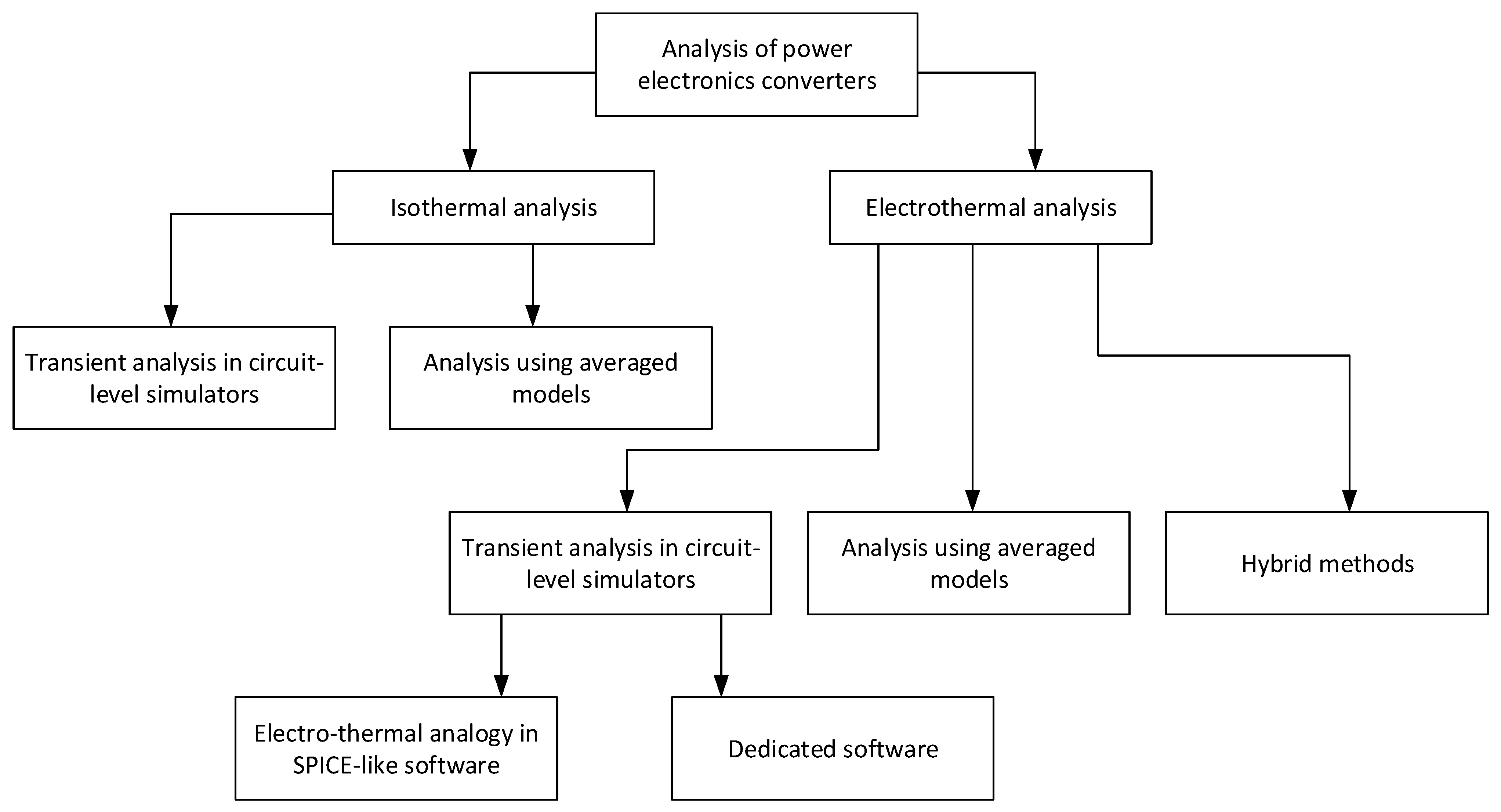
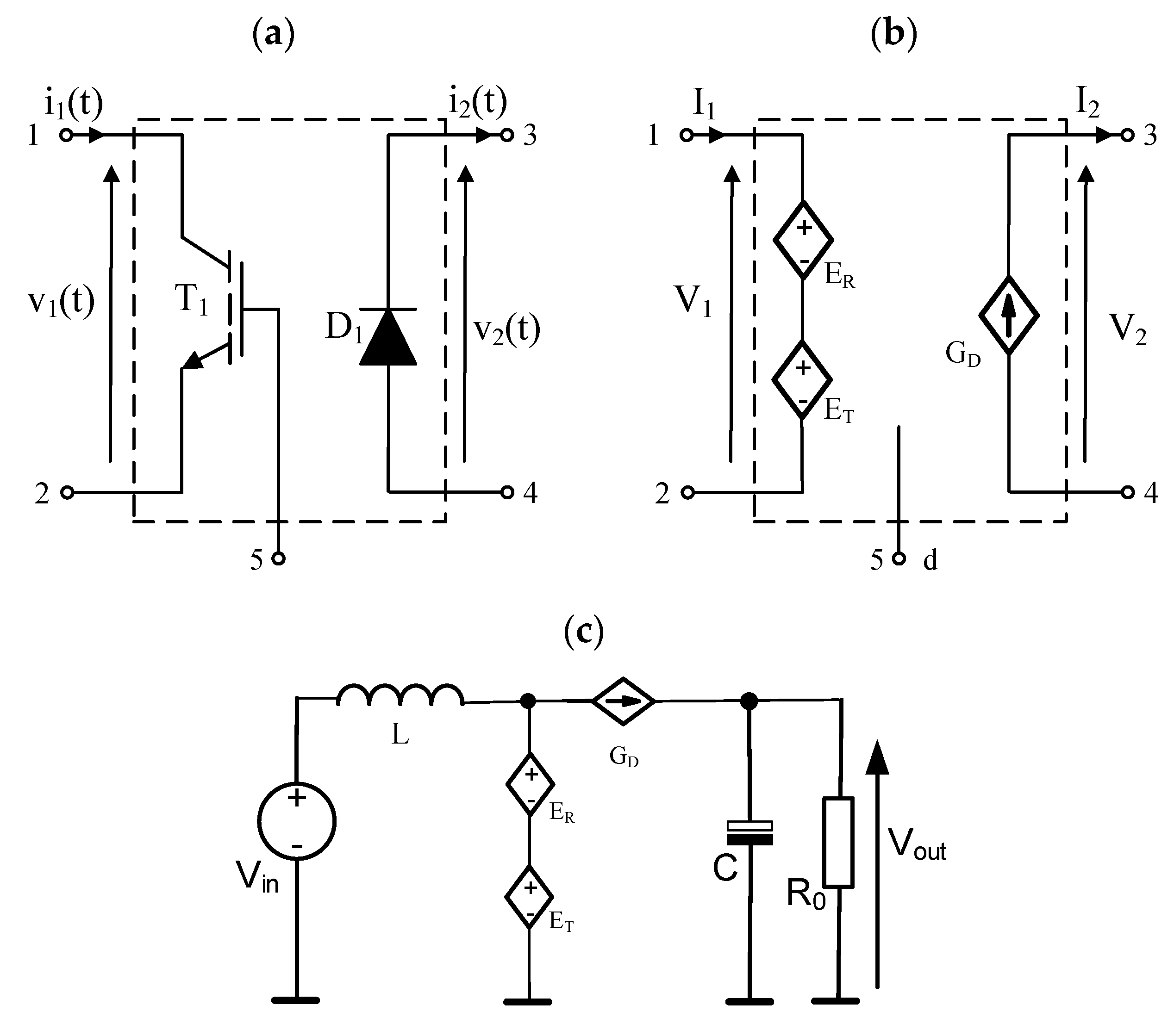
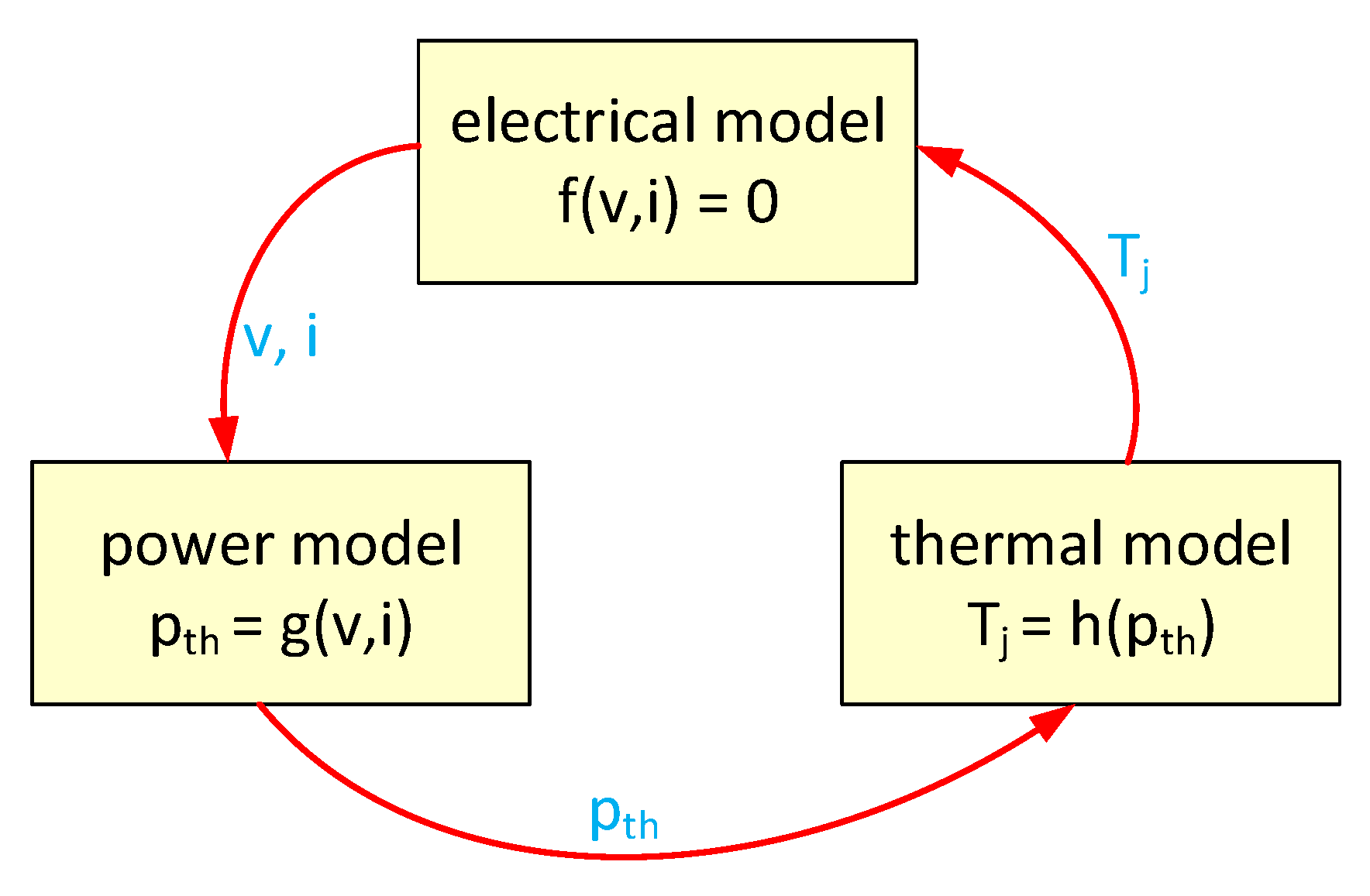
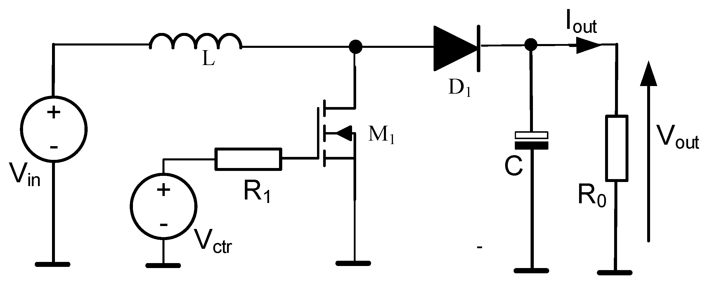
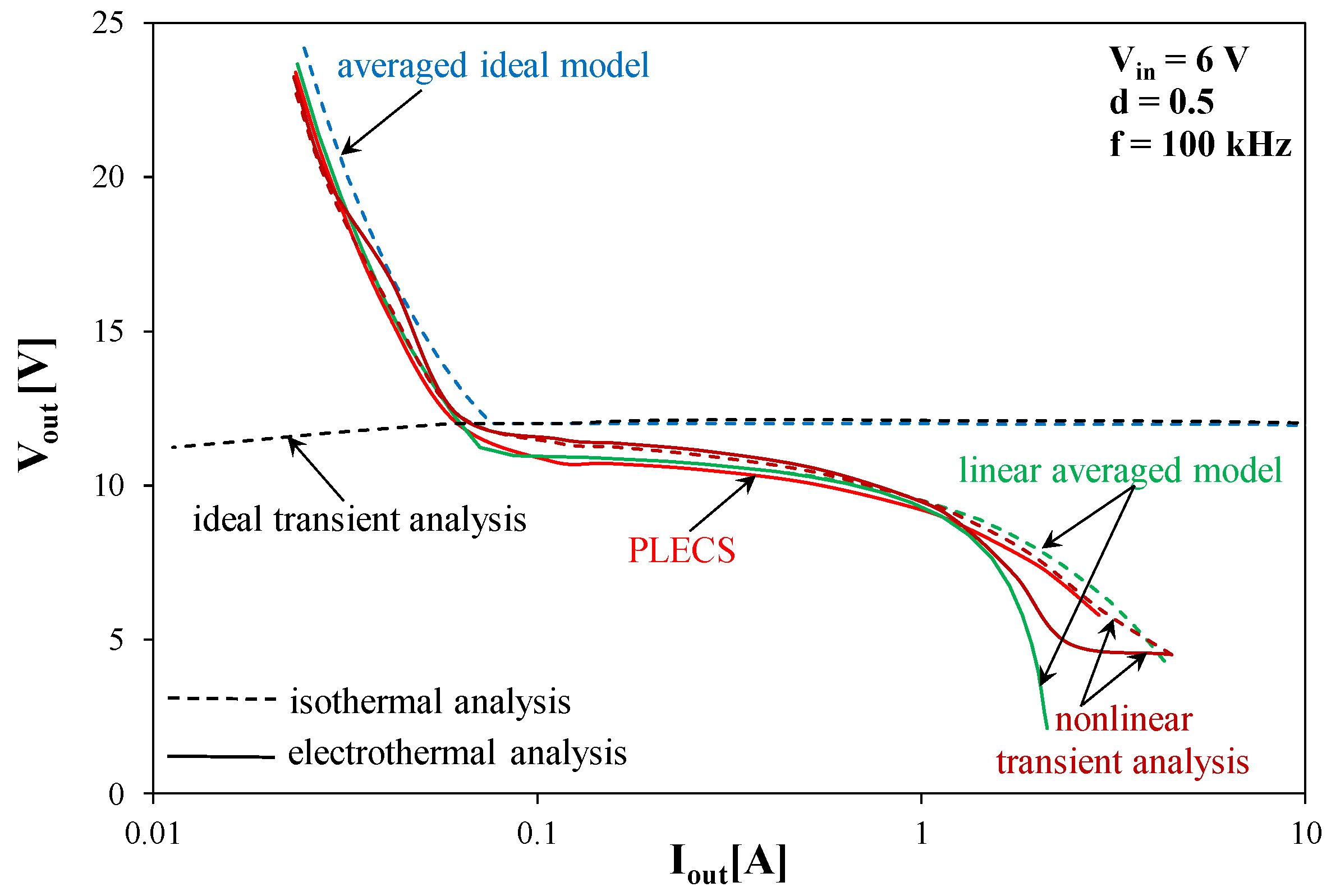
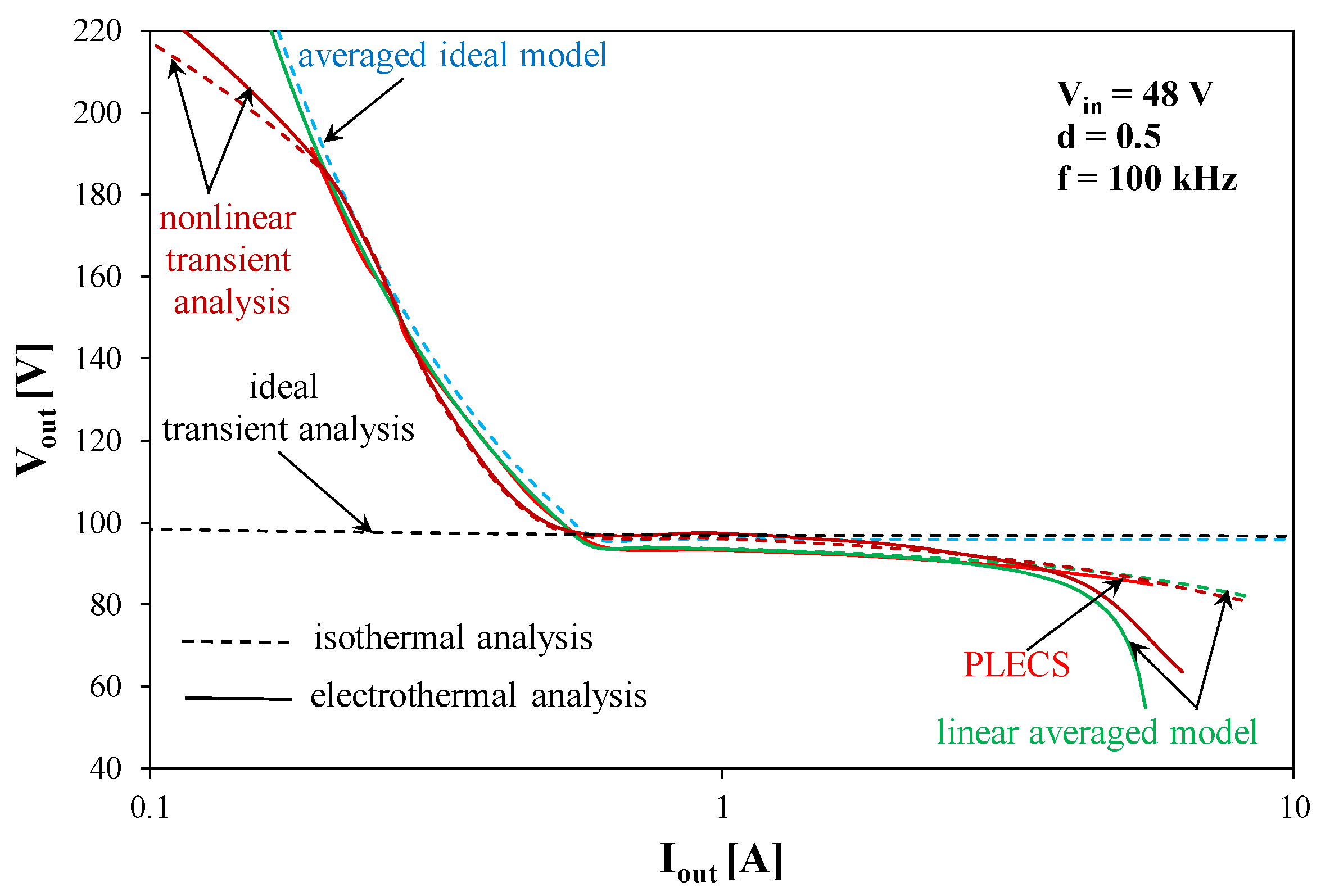
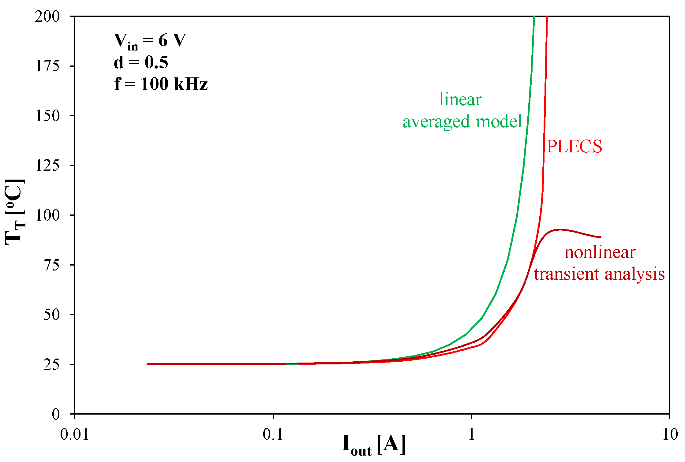
Table 1.
Properties of the methods of the isothermal transient analysis.
| Analysis Method | Ref. | Models of Semiconductor Devices | |||
|---|---|---|---|---|---|
| Ideal Switches | Piece-Wise Linear Models | Nonlinear Models | Electrical Inertia | ||
| Memoryless convolution | [27,28] | No | Yes | No | No |
| ASP with ideal switches | [3,7,30,31,32,33] | Yes | No | No | No |
| ASP with bivalent resistors | [28,34,35] | No | Yes | No | No |
| Accelerated steady-state analysis | [42] | No | No | Yes | Yes |
| Fast analysis at the steady state | [45] | No | No | Yes | Yes |
Table 2.
Properties of the isothermal averaged models.
| Averaged Model | Ref. | Models of Semiconductor Devices | |||
|---|---|---|---|---|---|
| Ideal Switches | Piece-Wise Linear Models | Power Losses | Types of Analyses | ||
| Lossless model | [48,49] | Yes | No | No | DC |
| Linear model with losses | [51,52,53,54,55,56] | No | Yes | Yes | DC |
| Ideal diode-transistor switch | [53,55] | Yes | No | No | AC, DC, transient |
| Nonideal diode-transistor switch | [3,24,34] | No | Yes | Yes | AC, DC, transient |
Table 3.
Properties of fast electrothermal analyses.
| Electrothermal Analysis Method | Ref. | Models of Semiconductor Devices | |||
|---|---|---|---|---|---|
| Piece-Wise Linear | Nonlinear | Electrical Inertia | Number of the Used Programmes | ||
| Transient analysis with shortened thermal time constant | [86] | No | Yes | Yes | 1 |
| Fast transient analysis with a convolution algorithm | [12] | No | Yes | Yes | 2 |
| Analysis in PSCAD | [88] | Yes | No | No | 1 |
| Analysis in PLECS | [13] | Yes | No | Yes * | 1 |
| Electrothermal averaged models | [50,89,90,92,93] | Yes | No | No | 1 |
| Electrothermal averaged models with switching losses | [91] | Yes | No | Yes | 1 |
| Electrothermal nonlinear averaged model | [94] | No | Yes | Yes | 1 |
| Hybrid method | [105,107] | No | Yes | Yes | 2 |
* only at calculations of dissipated power.
Table 4.
Duration time of the computations performed using selected methods.
| Averaged Models | Transient Analysis | |||
|---|---|---|---|---|
| Ideal Switches | Linear Switches | Ideal Switches | Physical Models | |
| Isothermal SPICE analysis | 0.02 s | 0.03 s | 50.3 s | 81.4 s |
| Electrothermal SPICE analysis | - | 0.03 s | - | 881.6 s |
| PLECS | - | - | - | 27 s |
Table 5.
Summary of the most important properties of the analysed methods of the analysis of DC–DC converters.
Table 5.
Summary of the most important properties of the analysed methods of the analysis of DC–DC converters.
| Method | Duration Time | Temperature Distribution | ΔT | Possible Electrical Analysis | Possibility of Experimental Verification | Difficulty Level of the Parameters Values Estimation Procedure | Number of the Used Simulation Programmes |
|---|---|---|---|---|---|---|---|
| Isothermal transient | Average | No | No | Transient | Yes | High | 1 |
| Isothermal averaged model | Very short | No | No | DC, AC | Yes | Low | 1 |
| Electrothermal transient in SPICE-like simulator | Very long | No | Yes | Transient | Yes | High | 1 |
| Electrothermal transient in dedicated software | Short | No | Yes | Transient, AC | Yes | Very low | 1 |
| Electrothermal averaged model | Very short | No | No | DC, AC | Yes | Low | 1 |
| Hybrid methods | Average/long | Yes | Yes | Transient, DC, AC | Limited | Very high | 2 or more |
Publisher’s Note: MDPI stays neutral with regard to jurisdictional claims in published maps and institutional affiliations. |
© 2021 by the authors. Licensee MDPI, Basel, Switzerland. This article is an open access article distributed under the terms and conditions of the Creative Commons Attribution (CC BY) license (https://creativecommons.org/licenses/by/4.0/).
Share and Cite
MDPI and ACS Style
Górecki, P.; Górecki, K. Methods of Fast Analysis of DC–DC Converters—A Review. Electronics 2021, 10, 2920. https://0-doi-org.brum.beds.ac.uk/10.3390/electronics10232920
AMA Style
Górecki P, Górecki K. Methods of Fast Analysis of DC–DC Converters—A Review. Electronics. 2021; 10(23):2920. https://0-doi-org.brum.beds.ac.uk/10.3390/electronics10232920
Chicago/Turabian StyleGórecki, Paweł, and Krzysztof Górecki. 2021. "Methods of Fast Analysis of DC–DC Converters—A Review" Electronics 10, no. 23: 2920. https://0-doi-org.brum.beds.ac.uk/10.3390/electronics10232920
Note that from the first issue of 2016, this journal uses article numbers instead of page numbers. See further details here.