DCRN: An Optimized Deep Convolutional Regression Network for Building Orientation Angle Estimation in High-Resolution Satellite Images

Abstract

Recently, remote sensing satellite image analysis has received significant attention from geo-information scientists. However, the current geo-information systems lack automatic detection of several building characteristics inside the high-resolution satellite images. The accurate extraction of buildings characteristics helps the decision-makers to optimize urban planning and achieve better decisions. Furthermore, Building orientation angle is a very critical parameter in the accuracy of automated building detection algorithms. However, the traditional computer vision techniques lack accuracy, scalability, and robustness for building orientation angle detection. This paper proposes two different approaches to deep building orientation angle estimation in the high-resolution satellite image. Firstly, we propose a transfer deep learning approach for our estimation task. Secondly, we propose a novel optimized DCRN network consisting of pre-processing, scaled gradient layer, deep convolutional units, dropout layers, and regression end layer. The early proposed gradient layer helps the DCRN network to extract more helpful information and increase its performance. We have collected a building benchmark dataset that consists of building images in Riyadh city. The images used in the experiments are 15,190 buildings images. In our experiments, we have compared our proposed approaches and the other approaches in the literature. The proposed system has achieved the lowest root mean square error (RMSE) value of 1.24, the lowest mean absolute error (MAE) of 0.16, and the highest adjusted R-squared value of 0.99 using the RMS optimizer. The cost of processing time of our proposed DCRN architecture is 0.0113 ± 0.0141 s. Our proposed approach has proven its stability with the input building image contrast variation for all orientation angles. Our experimental results are promising, and it is suggested to be utilized in other building characteristics estimation tasks in high-resolution satellite images.

1. Introduction

Remote sensing satellite data analysis plays an essential role in providing helpful information for urban planning and decision-making [1]. In addition, the recent sustainability research studies of smart cities depend on remote sensing data analysis [2]. Remote sensing data are presented in multi-modal form, e.g., aerial images, multispectral images, light detection and ranging (LiDAR) sensors, hyperspectral, and synthetic aperture radar (SAR) sensors [3]. The satellite image analysis is one of the most critical information analysis in satellite data [4]. Furthermore, human analysis - techniques for extracting building information are very tedious and inaccurate for the involvement of human expertise quality degree [5]. Therefore, computer-based systems are more accurate, save time, and save cost, especially in high-resolution satellite images. Computer vision is a computer-based image analysis system that utilizes image content information such as intensities, edges, textures, and morphological [6]. Such information is beneficial to enhance, segment, detect, or recognize objects inside these images. In the last decade, several computer vision algorithms were introduced for satellite image analysis applications [7].

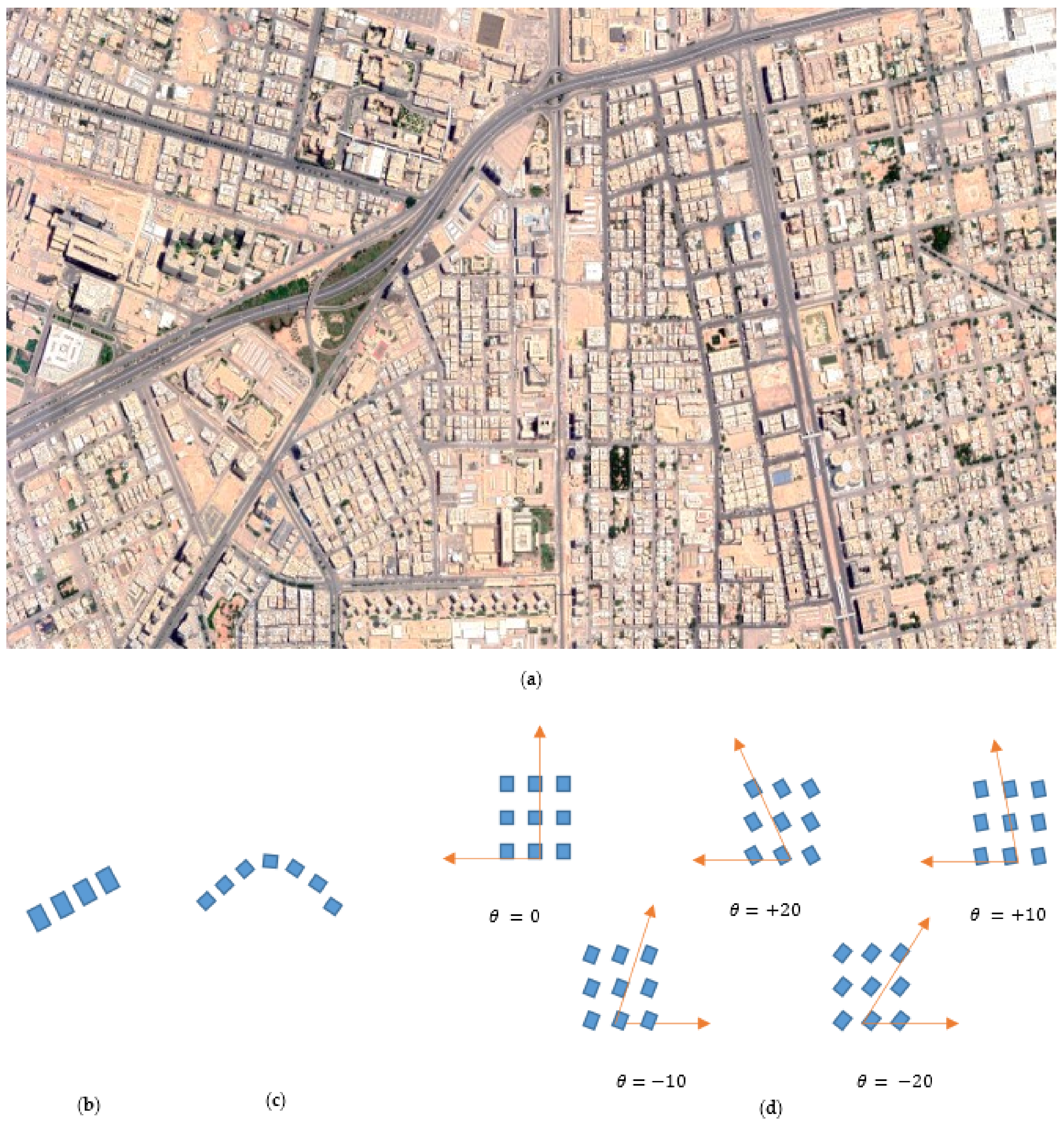
Automated building boundary extraction plays a crucial role in urban planning. The topographic data of building clusters are summarized into linear alignments, and non-linear alignments [8]. The linear alignments are divided into collinear, curvilinear, and align-along-road. The non-linear alignments are divided into grid and unstructured. These variations of building clusters inside urban planning make it challenging to accurately detect the angle of building orientation inside the satellite high-resolution images to obtain an optimum building boundary extraction. Therefore, the correct building orientation angle plays an essential role in the overall building detection algorithms. A sample of dense buildings satellite image at different building orientation angles (−20, 0, +10, +20) from Riyadh city is shown in Figure 1a. Different buildings alignments can be modeled such as linear as shown in Figure 1b, curvilinear as shown in Figure 1c and grid with different orientation angles as shown in Figure 1d. There are two main kinds of approaches for applying computer vision applications in satellite images, which are the traditional image processing approaches and deep learning approaches [9]. There is a challenge to employ recent approaches to analyze the building orientation angle.

Deep learning has been introduced by LeCun [10] as a subfield of artificial intelligence (AI), in which the computer algorithm learns tasks and distinguishes patterns with just constrained preparing information. Deep learning models can automatically extract the features with no need for feature extraction process [11]. Deep learning calculations learn designs by advancing through layers in a neural system to reach inferences. These advantages have made the utilization of deep learning a powerful tool in computer vision algorithms. Recently, deep learning shows exponential growing trend in compute vision tasks such as estimation [12], enhancement [13], segmentation [14], detection [15], and classification [16]. Deep learning is a powerful tool for a large amount of satellite image analysis tasks [17]. The deep learning algorithms have been employed in several satellite image analysis such as building detection [18], ship detection [19], vehicle detection [20], crop detection [21], and water detection [22]. There is a real need to employ deep learning to estimate some building characteristics in the remote satellite image.

This paper focuses on the building’s orientation angle as an essential characteristic for urban planning and automated building detection algorithms. Our proposed approach is based on the deep learning technique, which has proven its power compared with the traditional computer vision techniques. Deep learning is employed to estimate the angle of building orientation for buildings in Riyadh city collected during this study.

In this paper, our contributions are as follows:

(1)

We have proposed two deep learning approaches to estimate the building orientation angle in high-resolution satellite images.

(2)

The first approach based on deep transfer learning was examined using recent deep learning architectures.

(3)

The second approach is based on a lightweight deep learning architecture called DCRN to estimate building orientation angle.

(4)

A new early gradient layer has been proposed to overcome the drawbacks of building images and enhance the DCRN architecture performance.

(5)

A grid search hyper-parameters optimization has been applied to achieve the best performance for the DCRN architecture.

(6)

We have collected a dataset for Riyadh city that consisted of thousands of building images with different angles to achieve our task.

(7)

The two proposed approaches has been evaluated using our buildings dataset. Then, we compared our findings with the traditional and deep learning approaches in the literature.

The remainder of this paper is organized as follows. Section 2 presents the related works of building angle detection, including (1) traditional computer vision techniques, (2) deep learning techniques. Section 3 introduces our proposed material and methods in detail. Section 4 presents the experimental section with the proposed approach performance analysis with benchmarking against previous algorithms over our Riyadh-city building datasets. Section 5 introduces the discussion of our experimental results. Finally, the conclusion is introduced in Section 6.

2. Related Works

Buildings are one of the most important four patterns inside satellite images that need to be analyzed for optimum urban planning Zhang et al. [8]. Deep semantic segmentation for buildings received great attention last years Hatamizadeh et al. [23], Sun et al. [24], Yi et al. [25], Liu et al. [26], Abdollahi et al. [27], Yi et al. [25] and Wang and Li [28].

Another research dimension for building included the deep detection networks Shahin and Almotairi [29]. In Li et al. [30], the authors have introduced a building damage detection system based on deep learning. They have utilized the single-shot deep learning detector to detect the damaged area. They have utilized a Hurricane-Sandy dataset collected in 2012 in their study. The study has included only 350 images and achieved 77% average precision. In Zhang et al. [31], the authors have introduced a deep learning detection algorithm based on masked-RCNN. The authors have combined a fusion image to increase the system performance. The experiments have been applied to Chinese cities. The system achieved intersection over union (IOU) 87.8%. In Ma et al. [32], the authors have proposed a deep learning detection algorithm based on YOLOv3 for collapsed Buildings in Post-Earthquake. The dataset was collected after the 2008 Wenchuan and the 2010 Yushu earthquakes. The proposed algorithm reached 90.89% average precision.

However, these algorithms were employed for buildings area extraction alone. In addition, they neglected the other building characteristics which are essential in urban planning, such as height, orientation, and damage degree. Furthermore, the deep semantic segmentation techniques usually consume high processing time. The authors did not discuss the building orientation angle characteristic from a regression problem perspective, as challenging to construct a dataset for each building characteristic separately or transform the deep segmentation networks for other estimation tasks.

Several articles have been also introduced for buildings characteristics analysis such as building heights detection Liasis and Stavrou [33], building roof detection Nemoto et al. [34], building change detection More et al. [35], and building damage detection Li et al. [30]. Several estimation problems has been solved using deep learning approaches for buildings as shown in

Table 1. Various studies for building characteristics estimation in the literature.

Reference	Architecture	Processing Information	Estimation Task	Performance
Karatsiolis et al. [36]	Unet + Residual Network	Aerial RGB Images	Building Height Estimation	RMSE = 1.6
Li et al. [37]	Deep Regression Network	Remote Sensing RGB Images	Building Height Estimation	RMSE = 1.4
Liu et al. [38]	IM2ELEVATION Network	Aerial RGB images and Lidar data	Building Height Estimation	RMSE = 3.05
Cao and Huang [39]	M3Net Network	Multi views images and spectral images	Building Height Estimation	RMSE = 3.3
Sun et al. [40]	Fine-tuned MobileNet	Outdoor RGB Images	Building Orientation Estimation	Avg. Error = 23.63
Amini and Arefi [41]	Deep CNN	Remote Sensing RGB Images + Lidar data	Building Damage Estimation	Qulaity = 91.5%

. The buildings heights estimation has been deeply investigated in several previous works Karatsiolis et al. [36], Li et al. [37], Liu et al. [38], and Cao and Huang [39].

In Karatsiolis et al. [36], the authors introduced a deep learning model that combines architectural characteristics extracted through U-NET supported with residual connections and learned the height estimation by mapping the aerial RGB images. They achieved an RMSE value of 1.6. However, their model could not predict their heights in the DFC2018 dataset. In addition, the tall and thin buildings were rarely detected. The model sometimes failed to estimate their heights correctly. In some buildings cases, the model also failed to detect them. In Li et al. [37], the authors introduced a deep regression network that captured building height information with no need for multi-remote sensing perspectives. As a result, their model achieved the lowest RMSE value of 1.4. However, to achieve this target, they employed the ResNet architecture as a feature extractor backbone, then they fine-tuned the end of the network with a regression layer to fit the problem. In Liu et al. [38], the authors presented an IM2ELEVATION deep learning model based on the multi-sensor fusion of aerial RGB images and lidar data. They have achieved an RMSE value of 3.05. However, the network was very complex, which increased its inference time. Besides that, lidar data is not always available. In Cao and Huang [39], the authors introduced the M3Net deep learning model based on learning multi-spectral images, RGB images, and near-infrared bands. Moreover, they fed their network with multi-view images nadir, forward, and backward images). As a result, their model achieved an RMSE value of 3.3. Furthermore, their model was compared with single-task networks for height estimation, and they achieved a lower RMSE with the multi-task branching technique. However, the availability of all remote sensing information is challenging to be obtained for each city. In Sun et al. [40], the authors introduced an orientation estimation Network for outdoor RGB images. They have proposed a model based on fine-tuned MobileNet. They evaluated their model based on the average error, which was relatively high. Their dataset included buildings but not specifically for buildings images. In Amini and Arefi [41], the authors presented a deep CNN network to detect the collapsed buildings after an earthquake using height estimation. They employed both RGB images and lidar data pre-event satellite image as well as post-event. Their model was evaluated by overall quality metric which has achieved a value of 91.5%.

In this study, we focus on the building analysis in the high-resolution satellite image, especially the studies including building orientation angle calculation. Building orientation angle estimation is an active research point; there are three approaches in the previous studies to detect building boundaries involved with its orientation angle in high-resolution satellite RGB images. The first approach is based on the traditional image processing techniques. This approach has been proposed during building boundary detection, which is based on morphological binary processing. After binary thresholding of the building image, several pre-processing operations have been applied to remove artifacts. The major binary blob was utilized to extract the building boundary edges. Then, the orientation angle has been calculated as in Ghandour and Jezzini [42]:

$$cos\theta =\frac{\overrightarrow{V_1}·\overrightarrow{V_2}}{∥\overrightarrow{V_1}∥·∥\overrightarrow{V_2}∥}$$

(1)

where $\overrightarrow{V_1}·\overrightarrow{V_2}$ are two opposites vectors in the building and $\theta$ is the angle between them.

In Ghandour and Jezzini [42], the authors proposed a building boundary detection algorithm based on building shadow verification. They have utilized traditional image processing techniques for building roof boundary extraction. They utilized The SztaKi–Inria and Istanbul cities datasets. They have utilized a fusion idea to increase their system performance, which reached 95.8% of accuracy. However, the proposed algorithm lacked robustness in the case of changing the color nature of roof buildings. In Nguyen et al. [43], the authors have proposed an un-supervised automatic building detection algorithm based on an active contour algorithm. Their experiments have been applied on a dataset collected from Quebec City and Vaihingen City, Germany. The authors utilized LiDAR information to increase the system performance that reached 91.12% intersection of union (IOU).

The second approach is based on the Hough transform Wang et al. [3]. Hough lines in the Hough transform approach can detect the best fitting line from a set of 2-D points where each pixel in the spatial domain is represented into a sinusoidal curve in Hough space. The algebraic distance from the origin to the line ($\rho$) is defined as in Wang et al. [3]:

$$\rho =xcos\theta +ysin\theta$$

(2)

where (x; y) are coordinates of a point on the line in a Cartesian system, $\theta$ is the angle of the line’s normal with respect to the x-axis.

In Wang et al. [3], the authors have utilized the Hough transform approach for LIDAR information to extract the building boundary. Their experiments have been applied to three urban sites: Quantities Village site, Osaka city, and Toronto city. The average accuracy achieved through their proposed system has been 90%. In Bachiller-Burgos et al. [44], the authors have introduced a building boundary detection based on Hough transform. They have combined corners, segments, and polylines for the detected boundary. They have evaluated their proposed system based on qualitative analysis with no quantitative measurement of their proposed system.

The third approach is dependent on the supervised learning approach. In Kadhim and Mourshed [45], the authors have introduced a system for building heights detection based on traditional image processing. The authors have utilized graph fuzzy morphological processing to extract the building heights. The algorithm has been examined on seven urban sites in Cardiff, UK. They achieved a mean square error of the overall system reached 21%.

To our knowledge, in the literature, the building orientation angle has not been investigated through a deep learning framework as the main task. However, we have noticed that the learning of the object angle orientation based on deep learning has been discussed in the previous articles as a stage for arbitrary-oriented object detection Chen et al. [46], Wang et al. [47], and Tang et al. [48]. Their orientation estimation networks were based on VGG16 architecture. In Chen et al. [46], the authors investigated the buildings at three angles only. In Wang et al. [47], the authors introduced a ship detection model that neglected the evaluation of the ship’s orientation angle estimation accuracy. In Tang et al. [48], the authors investigated the vehicles orientation angle estimation in the vehicles detection model. However, the achieved RMSE value was very high and reached a value of 74.38. On the other hand, the convolutional regression networks have been previously introduced to estimate the orientation angles in several applications. In Hara et al. [49], the authors introduced a continuous object orientation estimation for pedestrians, which requires prediction of 0${}^{\circ }$ to 360${}^{\circ }$ degrees. In Phisannupawong et al. [50], the authors proposed a regression network based on Xception architecture for satellite orientation estimation from the image. However, they employed a simulated images dataset to train their model due to the insufficiency of dataset size. All these previous articles proved the efficiency of deep regression networks for the orientation angle estimation task.

On the other hand, there was a study to detect building orientation angles through SAR information Li et al. [51]. The authors proposed a mathematical model to estimate the building orientation angle from SAR information in several regions of interest. Their proposed system measured the overall building’s orientation angles inside each region of interest. However, there were several disadvantages of their proposed system. First, their results have been investigated using only the estimated angle’s mean and standard deviation values on limited case studies. Second, the high standard deviation values of the estimated angles of the buildings and the utilized dataset lacked uniform distribution of the buildings’ orientation angles which is more suitable for urban planning. Third, SAR information is produced by generating consequence pulses of radio waves to illuminate the target, and the space-based illuminators equipped with SAR radar lack the continuous availability of the transmitter to illuminate the target Maslikowski et al. [52].

Several drawbacks have been founded in the previous studies as follows: the dependency on the LIDAR sensor fusion with image information which increased system-processing complexity, the dependency on the traditional image processing for color building roof detection, which lacked robustness, the absence of building detection in a desert environment with no building roof color and low contrast image appearance. Furthermore, the high-resolution satellite RGB images can be captured instantly and provide separate data for each building information suitable for urban planning tasks. Such drawbacks could be tackled using deep learning approaches. In addition, all previous deep learning approaches for building detection neglected the building orientation angle as the main task. In the previous studies, building detection algorithms were involved with building orientation angle detection, which decreased the system performance Chen et al. [46]. Furthermore, the complexity of roof appearance made the prediction based on roof morphological appearance. Therefore, there is a complexity to modify the loss function of the deep learning detectors. However, the previous datasets lacked a dessert nature like in Saudi Arabia cities, which decreased the image contrast. Therefore, there is a real need to estimate the orientation angle of the building in remote sensing images in the desert environment.

3. Material and Methods

3.1. Material

We have collected a dataset for building images from three different high-resolution satellite images. The dataset of building images was collected from Riyadh city, Saudi Arabia. The size of each image was 50 MB in JPEG compression format with a resolution of $6140\times 8106$. Each image contained thousands of buildings with different orientation angles, locations, designs, roof shapes, and roof colors. The building images were cropped manually from each image. The total number of buildings were 15,190 building with different five angles (+20, +10, 0, −10, and −20) as shown in Figure 2. We have utilized the dataset-splitting technique to validate our proposed approach (80% training, 20% testing). We divided the collected building dataset into a 12,152 training set and a 3038 test set.

3.2. Methods

In this paper, we deliver two deep learning approaches for estimating the building angle orientation problem. The first approach is based on deep transfer learning, and the second is based on a novel optimized deep convolutional regression network.

3.2.1. Transfer Learning Approach

In this approach, we apply the fine-tuning of the pre-trained networks for the transfer learning approach [53], as shown in Figure 3. Thus, the proposed approach consists of input building images dataset, pre-processing, and fine-tuning stage.

The Building images dataset contains a wide building images dataset with predefined orientation angles. Each building image has its size, which varies according to the building size. Due to these variations, we need to set each building image to fit with the image input layer. The image input layer of each pre-trained network is as follows: AlexNet (227 × 227 × 3), VGG16 and VGG19 (224 × 224 × 3), GoogleNet (224 × 224 × 3), ResNet architectures (224 × 224 × 3), MobileNetv2 (224 × 224 × 3), and EfficientNet (224 × 224 × 3). We utilize several pre-trained networks (AlexNet, VGG16, VGG19,GoogleNet, ResNet, MobileNetv2, and EfficientNet). All of these networks have been trained on the ImageNet dataset [54]. ImageNet dataset contains hundreds of thousands of images for one thousand classes. Each pre-trained network has its learnable weights that can extract low, medium, and high-level features for any input image. We utilize the ability of such networks to extract edges, intensities variation, and contrast variation to distinguish the building orientation angle. All these networks consist of several convolutional layers that contain hundreds of learned kernels. Each pre-trained network has a different depth that means the number of layers deep in its architecture are as follows: AlexNet (8 layers deep), VGG16 (16 layers deep), VGG19 (19 layers deep), GoogleNet (22 layers deep), ResNet18 (18 layers deep), ResNet50 (50 layers deep), ResNet101 (101 layers deep), MobileNetv2 (53 layers deep), and EfficientNet (290 layers deep). However, these networks are fine-tuned by replacing their final layers that consist of a fully connected layer and Softmax classification layer with a single neuron fully connected layer and regression layer. Finally, each network is trained again to estimate the orientation angle from the input building image.

The transfer learning process is applied for our regression problem by transferring the learning task from the ImageNet dataset to our target building dataset. This process is defined as followed in Kandel and Castelli [53], each input image in a domain D consists of two components: features space F with a probability distribution $P\left(X\right)$ as in Equation (3):

$$D=\{F,P(X\left)\right\}$$

(3)

The source domain dataset $\left(D_S\right)$ can be defined as in Equation (4):

$$D_S={\left\{\right(X}_{S_1},Y_{S_1}),{(X}_{S_2},Y_{S_2}),\cdots \cdots ,{(X}_{S_n},Y_{S_n}\left)\right\}$$

(4)

where S represents the source domain for learning samples $X=\{x_1,x_2,x_3\cdots ,x_n\}$ with size n, the source dataset $X_S=\{x_{S_1},x_{S_2}\cdots x_{S_n}\}ϵF_S$, and the corresponding source class label $y_S\in {\gamma }_S$ the source dataset labels.

The target domain dataset $\left(D_T\right)$ can be defined as in Equation (5):

$$D_T={\left\{\right(X}_{T_1},Y_{T_1}),{(X}_{T_2},Y_{T_2}),\cdots \cdots ,{(X}_{T_n},Y_{T_n}\left)\right\}$$

(5)

where T represents the target domain for learning samples $X=\{x_1,x_2,x_3\cdots ,x_m\}$ with size m, the target dataset $X_T$ = $\{x_{T_1},x_{T_2}\cdots x_{T_m}\}ϵF_T$, and the corresponding target class label $y_T\in {\gamma }_T$ the target dataset labels.

The new learning task K is defined as having two components: label space $\gamma$ and objective function $\phi$ (.), as in Equation (6):

$$K=\{\gamma ,\phi (.\left)\right\}$$

(6)

where K represents the new learning task: K = {$\gamma$, $\phi$ (.)}, n>> m.

3.2.2. Deep Building Regression Network (DCRN)

The proposed DCRN approach is a lightweight architecture, which includes a pre-processing layer, several convolutional units, a dropout layer, and a regression layer. In this study, we aim to develop the topology of DCRN deep learning architecture by optimizing its hyper-parameters. First, as shown in Algorithm 1, we initialize the DCRN network with initial hyper-parameters to obtain the best DCRN network depth and training optimization algorithm. Secondly, we establish the hyper-parameters dictionary for the number dropout percentage (Drop Per.), initial learning rate, and the kernel size (KS) in each convolutional layer. Finally, the grid search algorithm is applied to obtain the best hyper-parameters for DCRN architecture.

Algorithm 1: Grid Search algorithm for our proposed DCRN approach.

Initialize the DCRN network with initial hyper-parameters.  Obtain the best training optimization algorithm for the DCRN network.  Obtain the best depth for the DCRN network.  Create the DCRN network.  Specify the hyper-parameters dictionary   KS = [3, 5, 7]   Drop Per. = [0.1, 0.2, 0.3, 0.4, 0.5]   Initial learning rate = [0.001, 0.002, 0.003, 0.004, 0.005]  For (n ∈ Iterations Number)   Start Grid Search Algorithm (n, Hyper-parameters Dictionary)  Output: Optimized DCRN Network that achieved the lowest RMSE.

Our proposed Deep Building Regression Network (DCRN) network is presented in Figure 4. It consists of a deep network input layer, a scaled gradient (SG) layer, three convolutional units, a dropout layer, a fully connected layer, and a regression layer. Convolutional unit1 consists of a convolutional layer, a batch normalization layer, and an activation layer. Convolutional unit 2, where each one consists of a convolutional layer, a batch normalization layer, an activation layer, an average-pooling layer, two repetitive convolutional unit3 where each one consists of a convolutional layer, a batch normalization layer, and an activation layer.

The image input layer contains two pre-processing stages, the first stage is resizing the input image with (64 × 64), and the second stage is converting the color input image to a gray-scale level to decrease the computational processing time as in Equation (7) [55].

$$PImage=0.299\ast R+0.587\ast G+0.114\ast B$$

(7)

where PImage represents the output image and R is the red channel of the input image, G is the green channel of the input image, and B is the blue channel of the input image.

In this paper, we employ the scaled gradient (SG) layer to enhance the building’s appearance and remove the shadow artifacts surrounded by the building. First, the gradient is utilized to highlight the edges of the building. Then, the histogram equalization of the input image is calculated to enhance the input image and remove lighting conditions variation. However, there is a building image lighting variation. Therefore, the scaling factor is added to the histogram equalization process to be adaptive [53]. The advantage of using the SG layer is shown in Figure 5. In this paper, we modify the scaling factor to be a learnable parameter inside the SG layer.

The proposed SG layer is defined as follows: we compute the gradient image Xs by convolving the input grayscale image by the gradient G:

$$Xs=PImage\ast G$$

(8)

where G is the gradient kernel defined as:

$$G=¼\ast \left[\begin{array}{ccc}1& 0& 1\\ 0& -4& 1\\ 1& 0& 1\end{array}\right]$$

Then, $X_g$ is the subtraction of input image and the gradient output image

$$X_g=PImage-Xs$$

(9)

The histogram-equalized image ${Eq\_X}_g$ is obtained by:

$${Eq\_X}_g=histeq\left(Xg\right)$$

(10)

where histeq is the histogram equalization function of the input image $Xg$. Finally, the scaled gradient output (SGimage) is defined as in Equation (11):

$$SGimage=\alpha . {Eq\_X}_g+Xs$$

(11)

where $\alpha$ is a scaling factor that is learned through training with range [0, 1].

The convolutional layer contains several convolutional kernels that are responsible for obtaining the features. These kernels are applied in a spatial area of the image to construct a receptive field. Each input image is divided into blocks and the kernels that contain learnable parameters convolving them. A single convolution process is defined as in Equation (12):

$$F_I^K=I_{x,y}\ast K_I^k$$

(12)

where $I_{x,y}$ represent input image (x, y), $K_I^k$ represents Ith convolutional kernel of kth layer.

Batch normalization (BN) improves deep learning stability and accelerates the training process by eliminating internal covariate change. This process consists of normalizing the previous activation layer output and subtracting the mean of the batch. Then, dividing the output by the standard deviation of the batch. The batch normalization transformation function ($T_I^k)$ is defined in Equation (13).

$$N_I^k=\frac{T_I^k}{{\sigma }^2+{\sum }_i{T}_i^k}$$

(13)

where $N_I^k$ represents the feature map after the normalization process, $T_I^k$ represents the input feature map, and $\sigma$ represents variation through the feature map.

According to the massive number of computed parameters, a down-sampling process should be applied to the input features map. Therefore, we have utilized the averaging as in the following equation:

$$Z_I=f_p\left(F_{x,y}^I\right)$$

(14)

where $Z_I$ represents Ith output feature map, $F_{x,y}^I$ represents Ith input feature map, and $f_p$ represents pooling operation type.

The activation function is responsible for making the network decision. The rectified linear unit (Relu) activation function has two advantages: speed and robustness for the CNN learning process.

$$T_I^k=f_A\left(F_I^k\right)$$

(15)

$F_I^k$ represents the output of convolution layer operation, and $f_A$ represents the activation rectified linear unit (ReLU) function.

The dropout layer has proven its potential as a regularization technique in several deep learning architectures. It provides the regularization process during the learning process. This process is utilized to prevent over-fitting and achieved by stochastic dropping out some neurons during the training process.

The Fully connected (FC) layer consists of a single neuron for the estimated orientation angle value located before the final regression layer. Thus, Fc is responsible for remapping the feature map on a single neuron value.

The regression layer employs the loss function during the training process in supervised learning to obtain the best parameters. The most common regression loss function is the mean square error that represents the squared distances between the target variable $Y_i$ and the predicted values $Y_i^{{}^{\prime }}$ as in Equation (16).

$$MSE=\frac{1}{n}\sum _{i=1}^n{(Y_i-Y_i^{{}^{\prime }})}^2$$

(16)

Hyper-parameters play an essential role in the performance of deep networks. Each convolutional layer (CL) consists of number of kernels (K) with kernel size (KS). The learning rate value is utilized to achieve the minimum loss value with a relatively high convergence speed. Firstly, we select the hyper-parameters that have been utilized in similar works. We select the learning rate as followed in a similar direction estimation deep network [56]. The minimum batch size value was investigated in a similar remote sensing application [57] and the minimum batch size 64 has achieved the best average accuracy among several minimum batch sizes. The epochs number controls the network training iterations. In our estimation problem, about 30 epochs are utilized to achieve the minimum loss value. Therefore, we set the initial hyper-parameters for our proposed DCRN as shown in

Table 2. Hyper-parameters setting for our proposed DCRN network.

Layer Name	Initial Hyper-Parameters	Optimized Hyper-Parameters
CLs in Convolutional Unit 1	KS [3, 3], K = 64	KS [7, 7], K = 64
CLs in Convolutional Unit 2	KS [3, 3], K = 128	KS [7, 7], K = 128
	KS [3, 3], K = 256	KS [7, 7], K = 256
	KS [3, 3], K = 512	KS [7, 7], K = 512
CLs in Convolutional Unit 3	KS [3, 3], K = 1024	KS [7, 7], K = 1024
	KS [3, 3], K = 1024	KS [7, 7], K = 1024
Activation Layers	Relu Unit	Relu Unit
Pooling Layers	KS [2, 2], stride = 2	KS [2, 2], stride = 2
Dropout Layers	Drop Percentage = 20%	Drop Percentage = 30%

as follows: the KS to the lower value 3, the dropout percentage to 20% of neurons drop, and the initial learning rate to 0.001. Secondly, during the experiments, we investigate the optimized hyper-parameters for our proposed DCRN architecture using an exhaustive grid search method [58] as shown in Algorithm 1. Our DCRN architecture has achieved the best performance with the following parameters: the KS to the value 7, the dropout percentage to 30% of neurons drop, and the initial learning rate to 0.004.

4. Results

We perform our proposed system based on MATLAB 2020a. The system platform contains Quad-Core 2.9 GHz Intel i5 with 16 GB RAM. The GPU computation is done through NVIDIA Quadro 5000 with 16 GB internal RAM and computing capability 6.1. We design seven main experiments to prove our findings as follows: (1) We investigate the performance of our first proposed approach, (2) We investigate the best depth for our proposed DCRN architecture, (3) We investigate the SG layer effect on DCRN architectures with different optimization algorithms, (4) We investigate the performance of DCRN architecture after the hyper-parameters grid-search optimization, (5) We compare between our optimized DCRN approach and the other methods in the literature, (6) We perform a computational cost analysis for our approach vs. the previous methods, and (7) We visualize several examples to answer how each algorithm makes its decision to estimate the correct orientation angle.

In this section, we assess our experimental results based on quantitative and qualitative results. We use the root mean square error (RMSE) value as defined in Equation (17), mean absolute error (MAE) as defined in Equation (18) and Adjusted R-Squared value as defined in Equation (19). Furthermore, we perform a computational cost analysis for our proposed DCRN network. On the other hand, we visualize the learning curves for both training and validation cycles for our proposed DCRN network. In addition, we visualize the activation of our proposed DCRN network.

$$\mathrm{RMSE}=\sqrt{\frac{1}{n}\sum _{i=1}^n{({\theta }_i-{\theta }_i^{{}^{\prime }})}^2}$$

(17)

$$\mathrm{MAE}=\left(\frac{1}{n}\right)\sum _{i=1}^n\left|{\theta }_i-{\theta }_i^{{}^{\prime }}\right|$$

(18)

$$\mathrm{Adjusted} \mathrm{R\_Squared}=\frac{(1-\mathrm{R\_Squared})(n-1)}{(n-k-1)}$$

(19)

where

$$\mathrm{R\_Squared}=1-\frac{\sum {\theta }_i-{\widehat{\theta }}_i}{\sum {\theta }_i-{\widehat{\theta }}_i}$$

(20)

where ${\theta }_i^{{}^{\prime }}$ is the predicted building orientation angle for instance i, ${\theta }_i$ is the correct building orientation angle for instance i with a given n samples of the test dataset. K is the number of independent variables.

4.1. Experiment 1

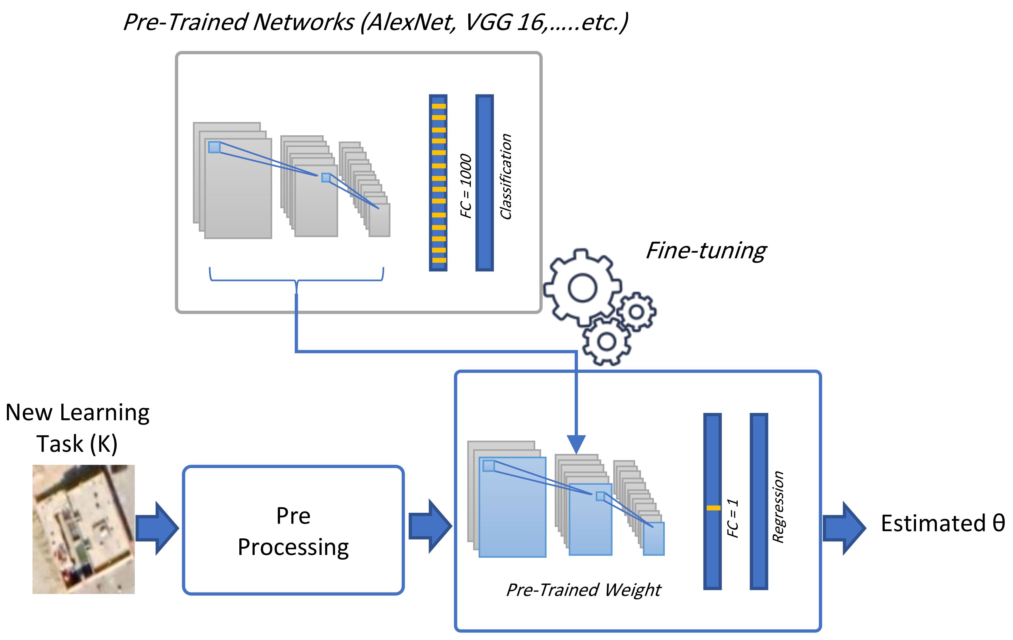
In this experiment, we investigate the transfer learning approach, as shown in Figure 3. We utilize AlexNet, VGG16, VGG19, GoogleNet, ResNet18, ResNet50, ResNet101, MobileNetV2, and EfficientNet. We employ the RMSE value to compare different pre-trained networks. We have also compared two optimization algorithms during this experiment: adaptive moment estimation (ADAM) and root mean square (RMS). ALL network training parameters are set as follows: learning rate: 0.001, epochs: 30, minimum batch size: 64. As shown in

Table 3. The achieved RMSE values with our proposed transfer learning approach for building angle orientation estimation.

Optimizer	AlexNet	VGG16	VGG19	GoogleNet	ResNet18	ResNet50	ResNet101	MobileNetV2	EfficientNet
ADAM	5.06	147.48	103.14	2.22	2.31	2.67	2.65	2.14	2.18
RMS	4.21	78.98	34.5	2.45	2.44	2.76	2.58	2.43	2.44

, MobileNetV2 has achieved the lowest RMSE value (2.14) with ADAM optimizer and (2.43) with RMS optimizer. EfficientNet has achieved the second rank of the RMSE value (2.18) with RMS optimizer and (2.44) RMSE value with ADAM optimizer. ALL ResNet architectures have achieved low RMS values as follows: ResNet18 (2.31) RMSE value with ADAM optimizer and (2.44) RMSE value with RMS optimizer, ResNet50 (2.67) RMSE value with ADAM optimizer and (2.76) RMSE value with RMS optimizer, and ResNet101 (2.65) RMSE value with ADAM optimizer and (2.58) RMSE value with RMS optimizer. AlexNet has achieved a high RMSE value (5.06) with the ADAM optimizer and (4.21) RMSE value with the RMS optimizer. On the contrary, both VGGNet models have achieved the worst RMSE values. VGGNet16 has achieved the highest RMSE value (147.48) with ADAM optimizer and (79.98) RMSE value with RMS optimizer. VGGNet19 has achieved a high RMS value (103.14) with ADAM optimizer and (34.5) RMSE value with RMS optimizer.

4.2. Experiment 2

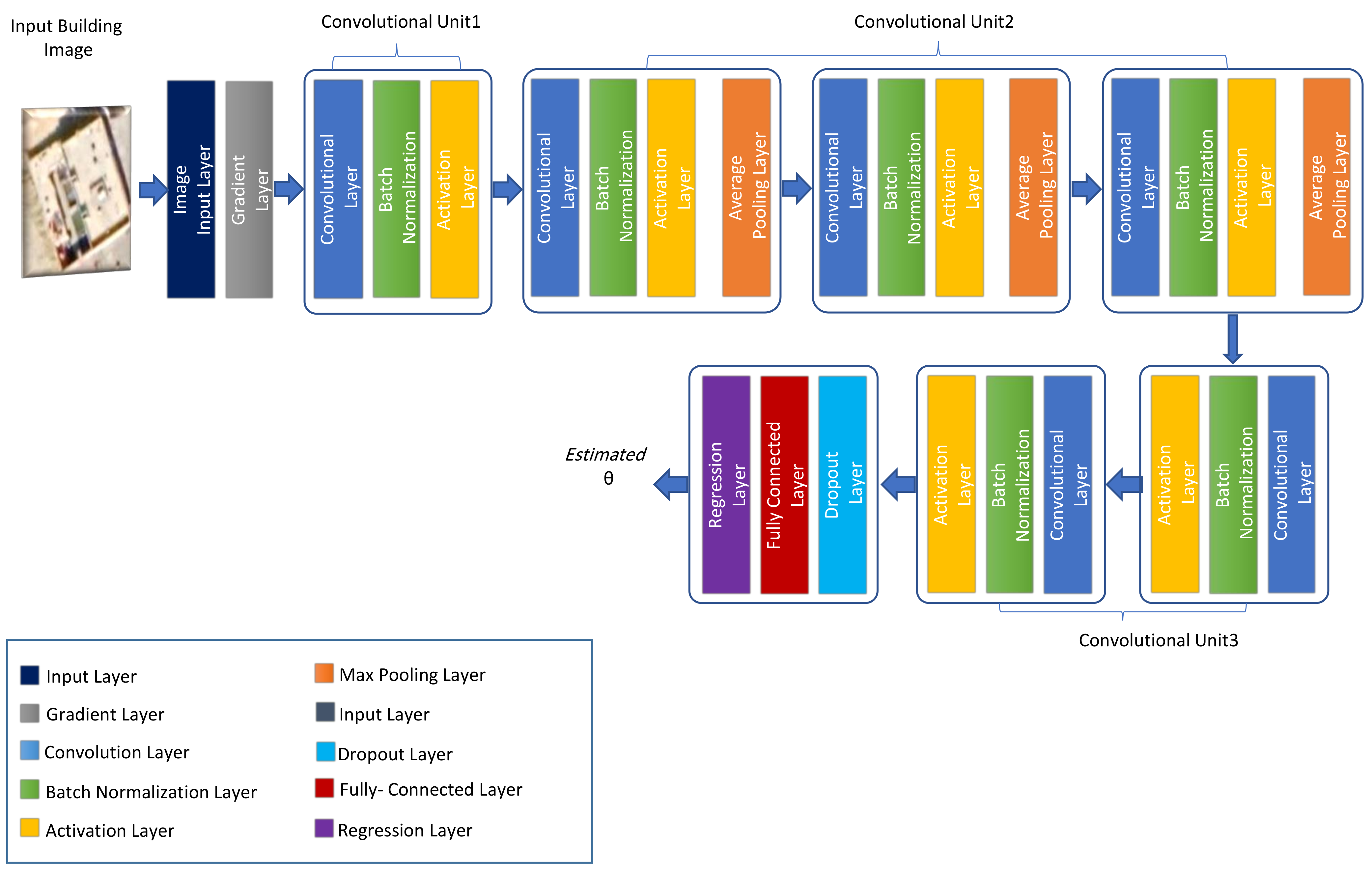
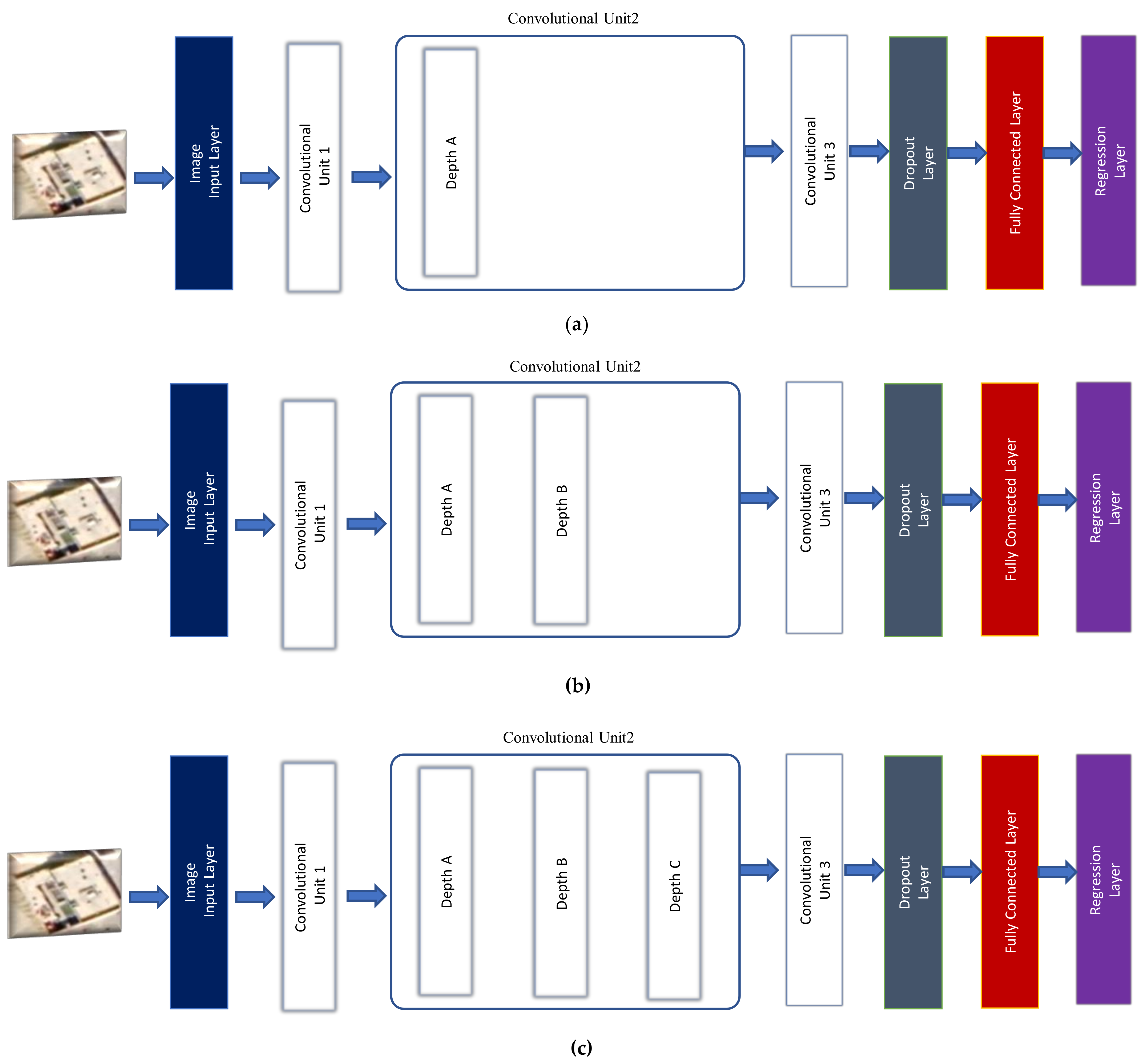
In this experiment, we investigate the performance of the second proposed DCRN approach. The network’s depth is considered an important parameter to determine the network performance. Therefore, we investigate the depth of convolutional unit 2 variation. This experimental setup utilizes the RMSE value to compare different depths, as shown in Figure 6. The network training parameters setup is as follows: learning rate: 0.001, epochs: 30, minimum batch size: 64.

Figure 6 shows the details of variation of convolutional unit 2 in its depth. We keep the remind of DCRN fixed without using the SG layer.

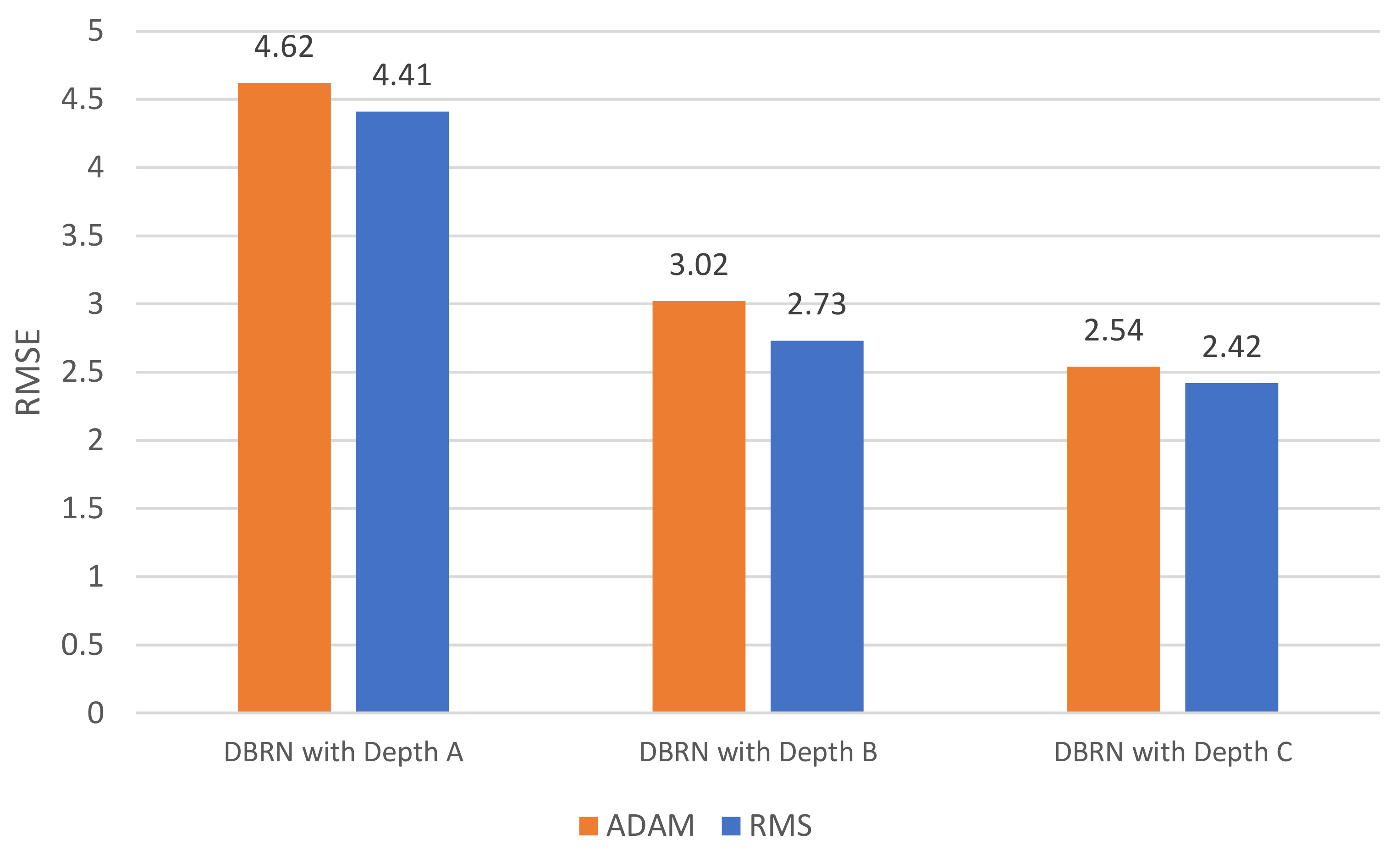
As shown in Figure 7, the DCRN with depth A has achieved the highest RMSE values with both utilized optimizers. The ADAM optimizer has achieved 4.62 RMSE value and RMS has achieved 4.41 RMSE value.DCRN with depth B has achieved 3.02 with ADAM optimizer and has achieved 2.73 with RMS optimizer. The lowest RMSE values have been achieved by using DCRN with depth C. The DCRN architecture with depth C has achieved 2.54 with ADAM optimizer and has achieved 2.42 with RMS optimizer.

4.3. Experiment 3

In this experiment, we investigate the SG layer effect on the proposed DCRN architecture. The network training setup is as follows: learning rate: 0.001, minimum batch size: 64, and epochs: 30. As shown in

Table 4. The RMSE values for DCRN approach with SG Layer based on different optimizers.

	RMSE Value	Adjusted R-Squared Value
DCRN with ADAM Optimizer	1.9372	0.9025
DCRN with RMS Optimizer	1.8914	0.9104

, the proposed DCRN has achieved the RMSE value (1.8914) using the RMS optimizer. However, the proposed DCRN has achieved an RMSE value (1.9372) using the ADAM optimizer. The RMS optimizer has achieved the Adjusted R-squared value (0.9104). However, the ADAM optimizer has achieved the lowest Adjusted R-squared value (0.9025) with our proposed DCRN architecture.

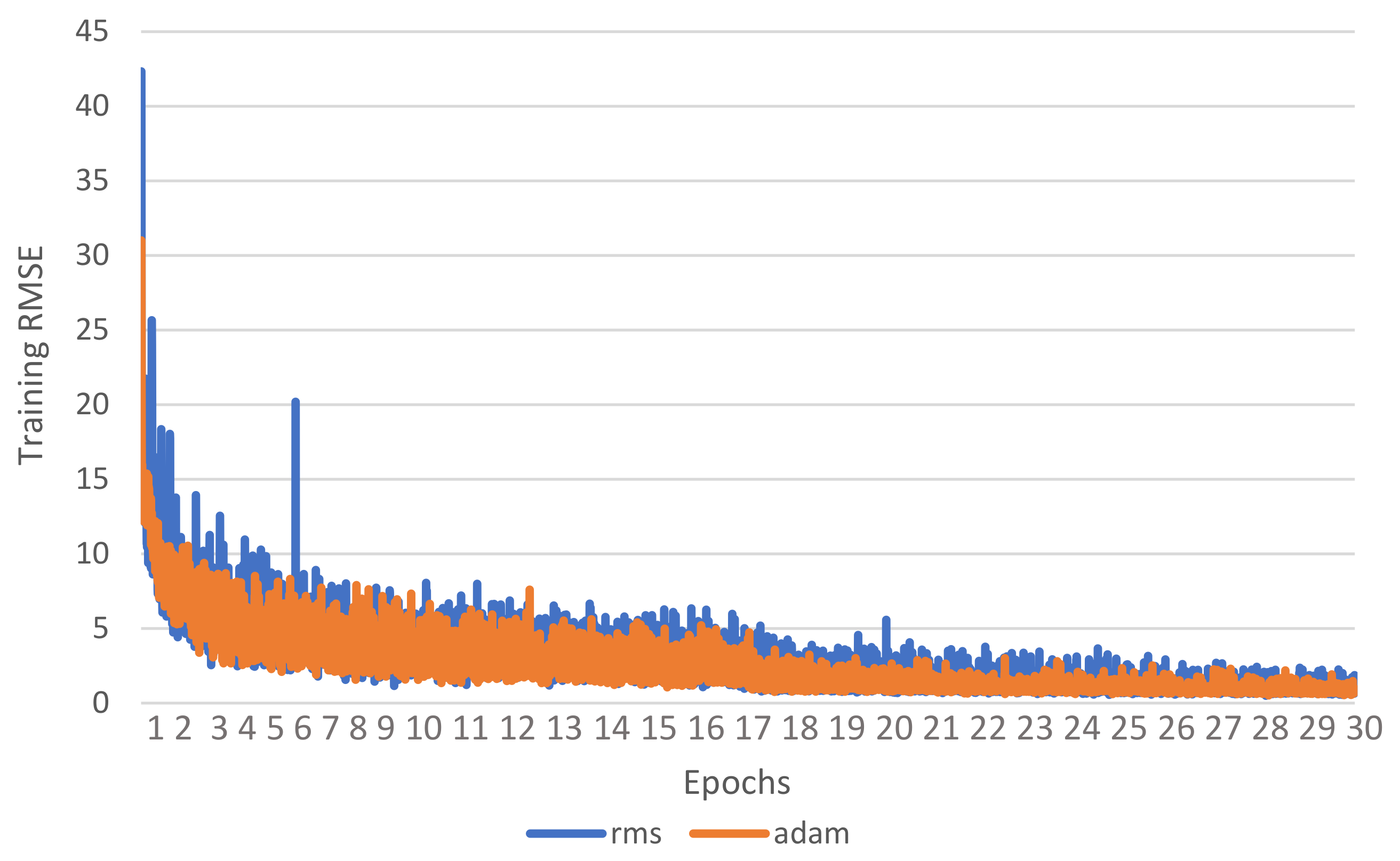
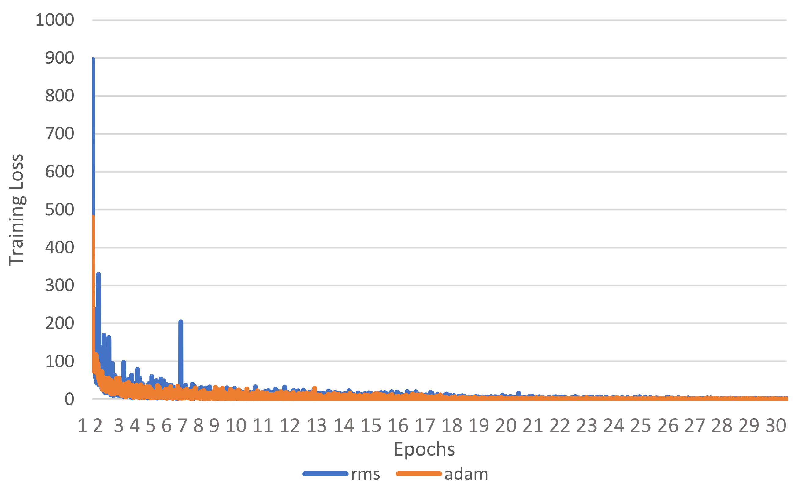
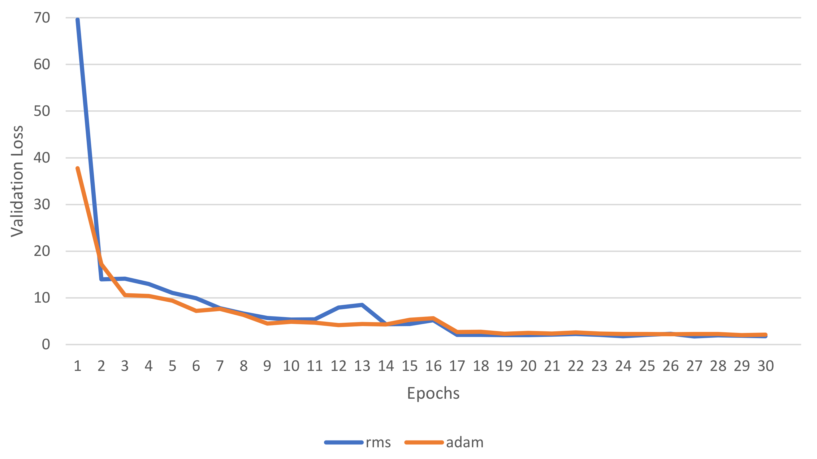
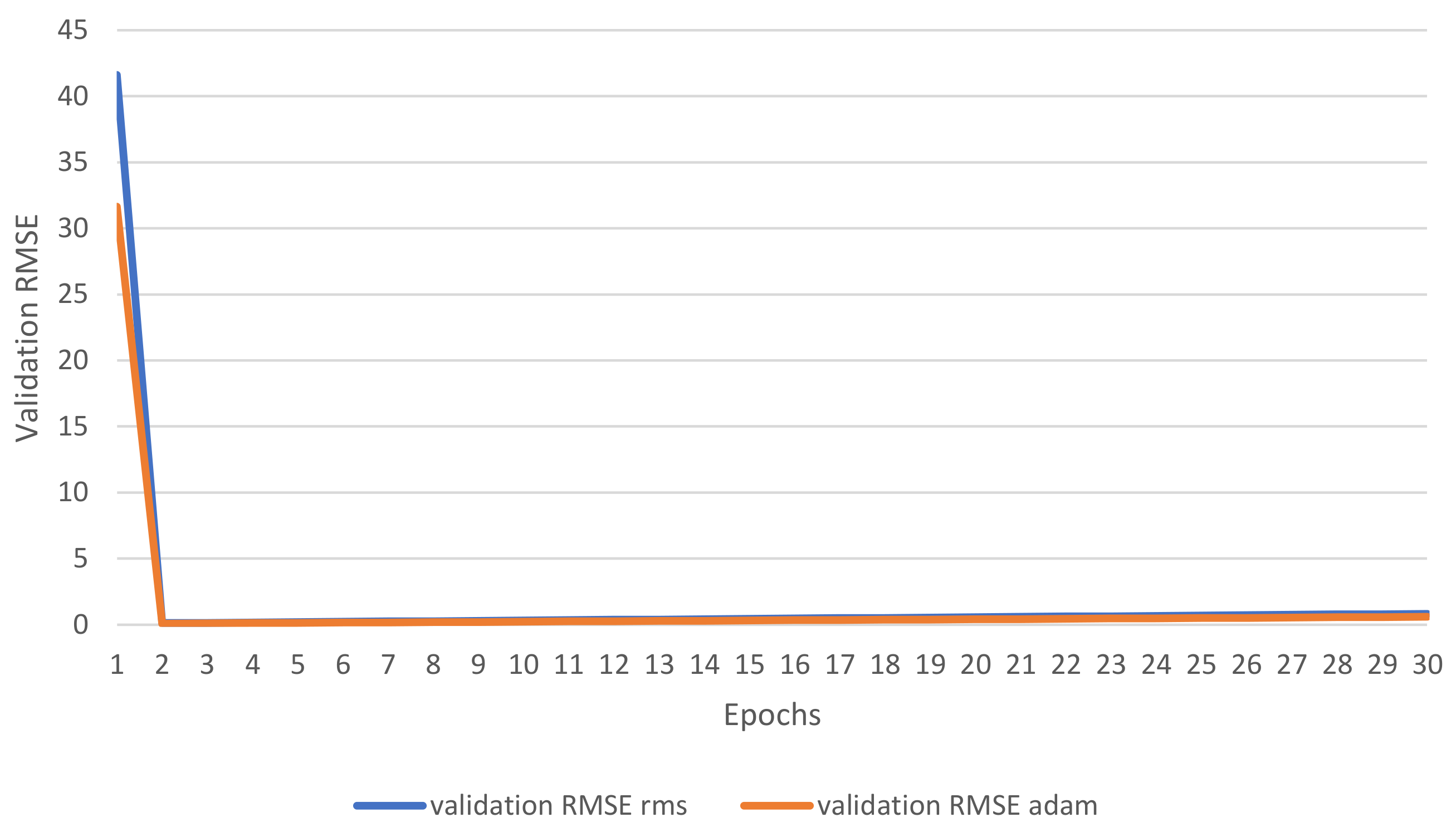
Also, in this experiment, we investigate both loss and RMS learning curves using our proposed SG layer with the architecture of depth c based on RMS and ADAM optimizers. The loss and RMS for the training set are shown in Figure 8 and Figure 9. The loss and RMS for the validation set are shown in Figure 10 and Figure 11.

We have noticed that both learning curves during the training cycle are oscillating and starting with high values as shown in Figure 8 and Figure 9. In Figure 10 and Figure 11, we visualize both learning curves during the validation cycle. In this experiment, the RMS optimizer loss and RMSE value have started highly during the first epochs However, the performance of both optimizers are very similar at the end of the epochs.

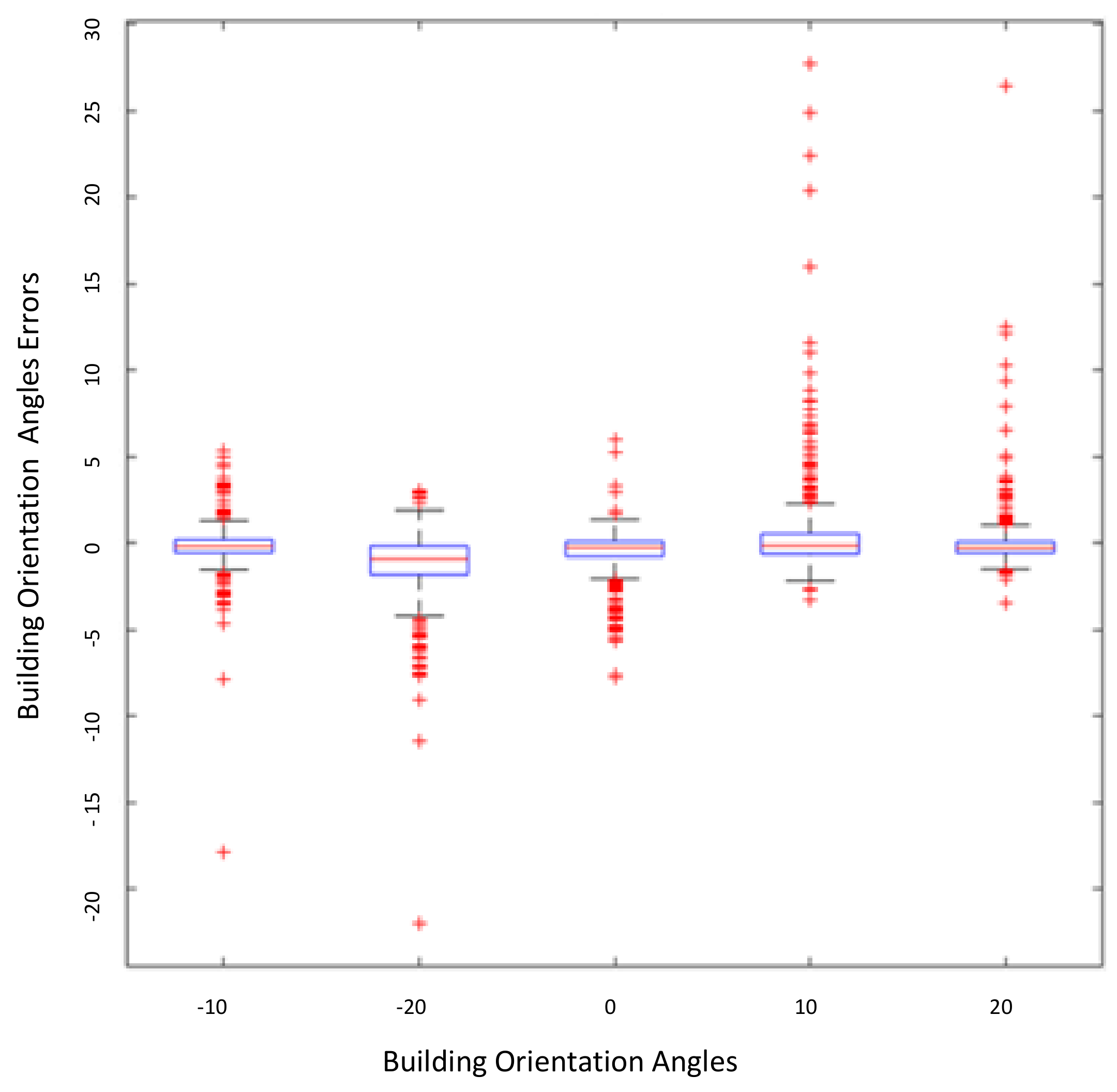
We visualize the residual plots of our proposed optimized DCRN approach for estimating the different building orientation angles as shown in Figure 12. The building orientation angle 0 has achieved the smallest boxplot with the lowest angle error variation between the angles. Similar boxplots are noticed for the estimation of angles (10, 20, and −10). However, the boxplots represent the estimation of (−20) angle is the largest boxplot. The angle 10 represents the largest variation between the angle’s errors.

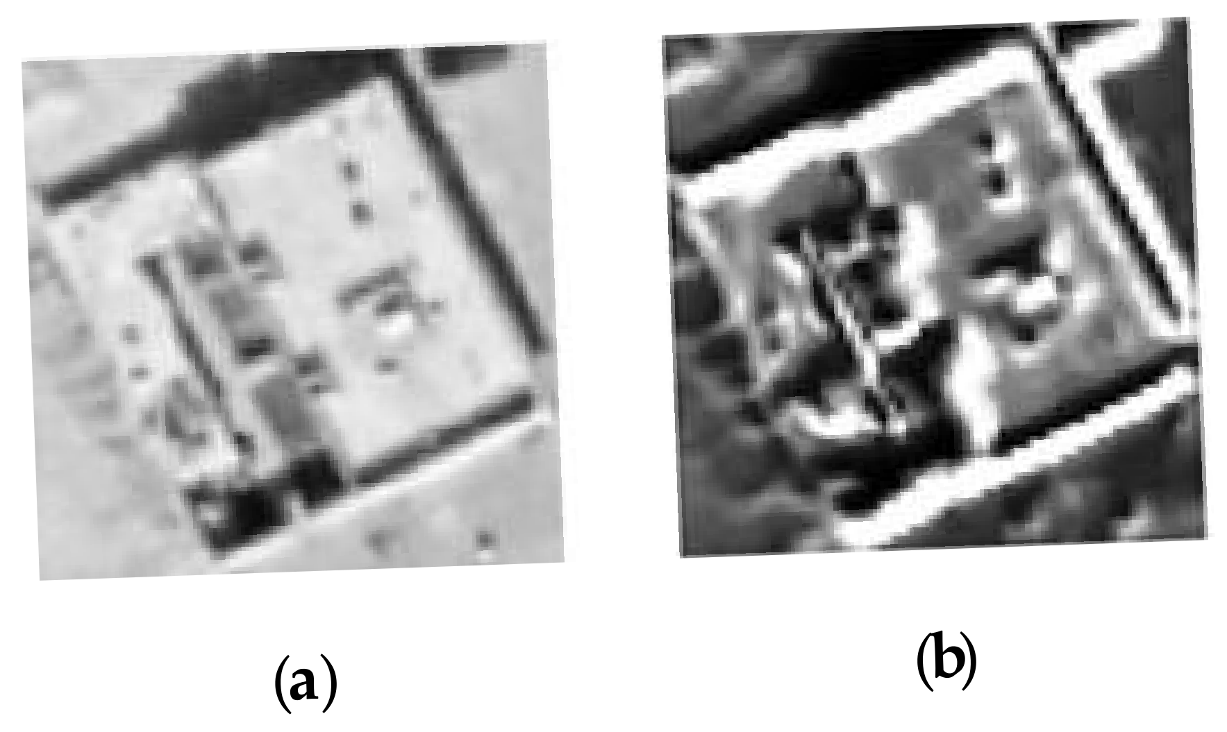
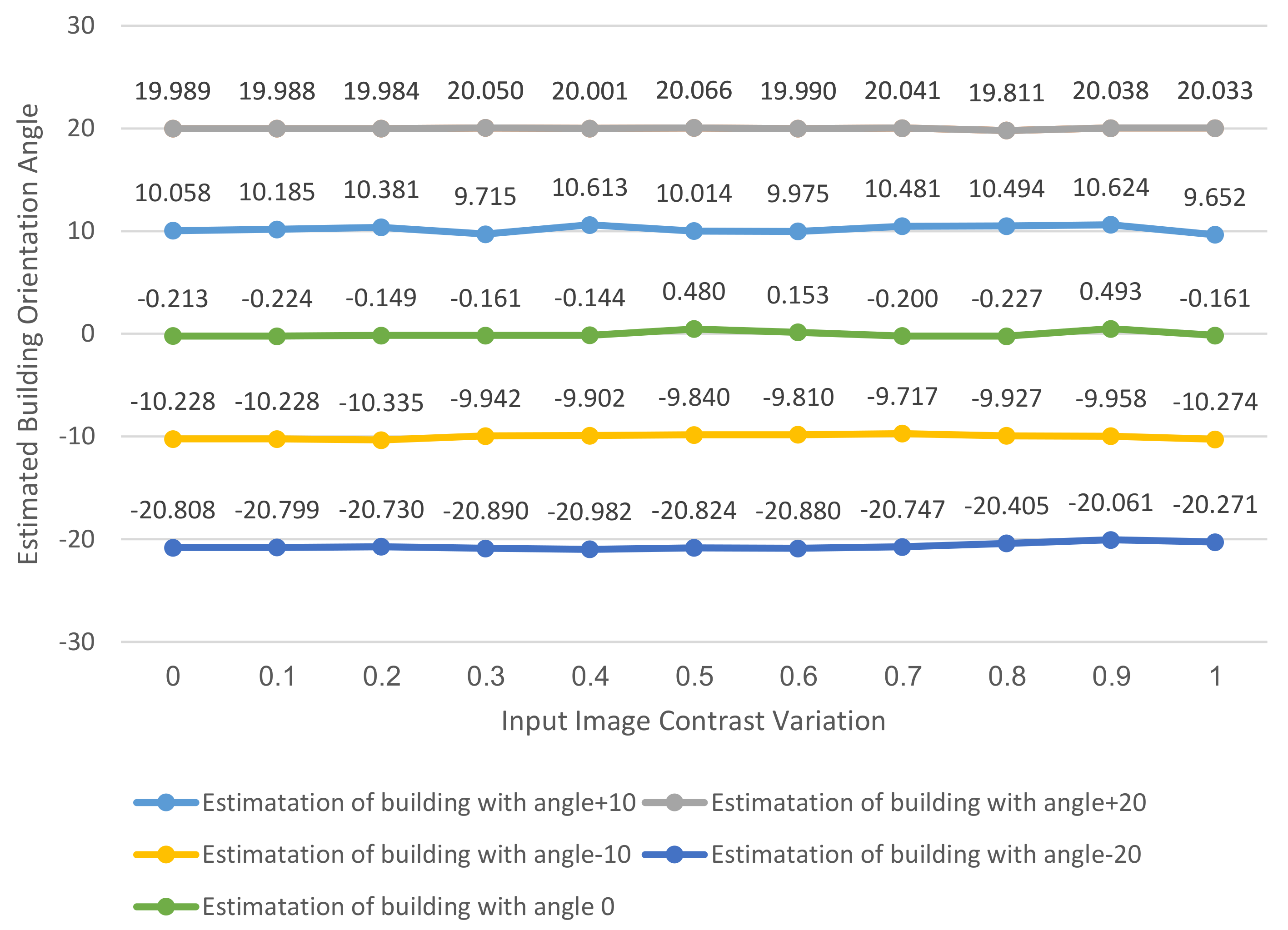
In this experiment, we visualize the robustness of our proposed method with the variation of the building image contrast as shown in Figure 13. We apply our proposed algorithm by simulating several contrast values in range [0–1]. The contrast variation is applied to the five angles in the test set.

4.4. Experiment 4

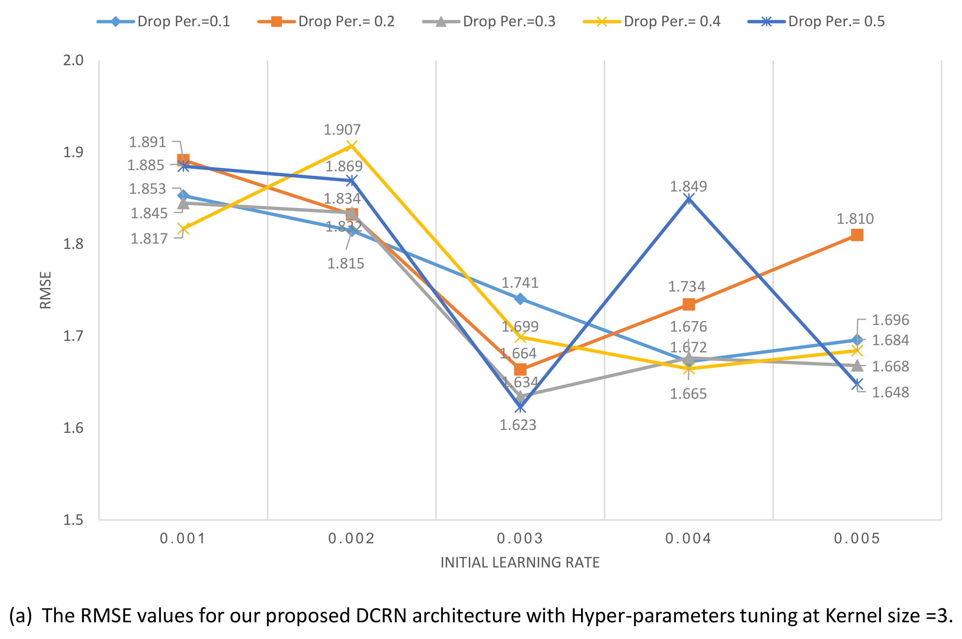
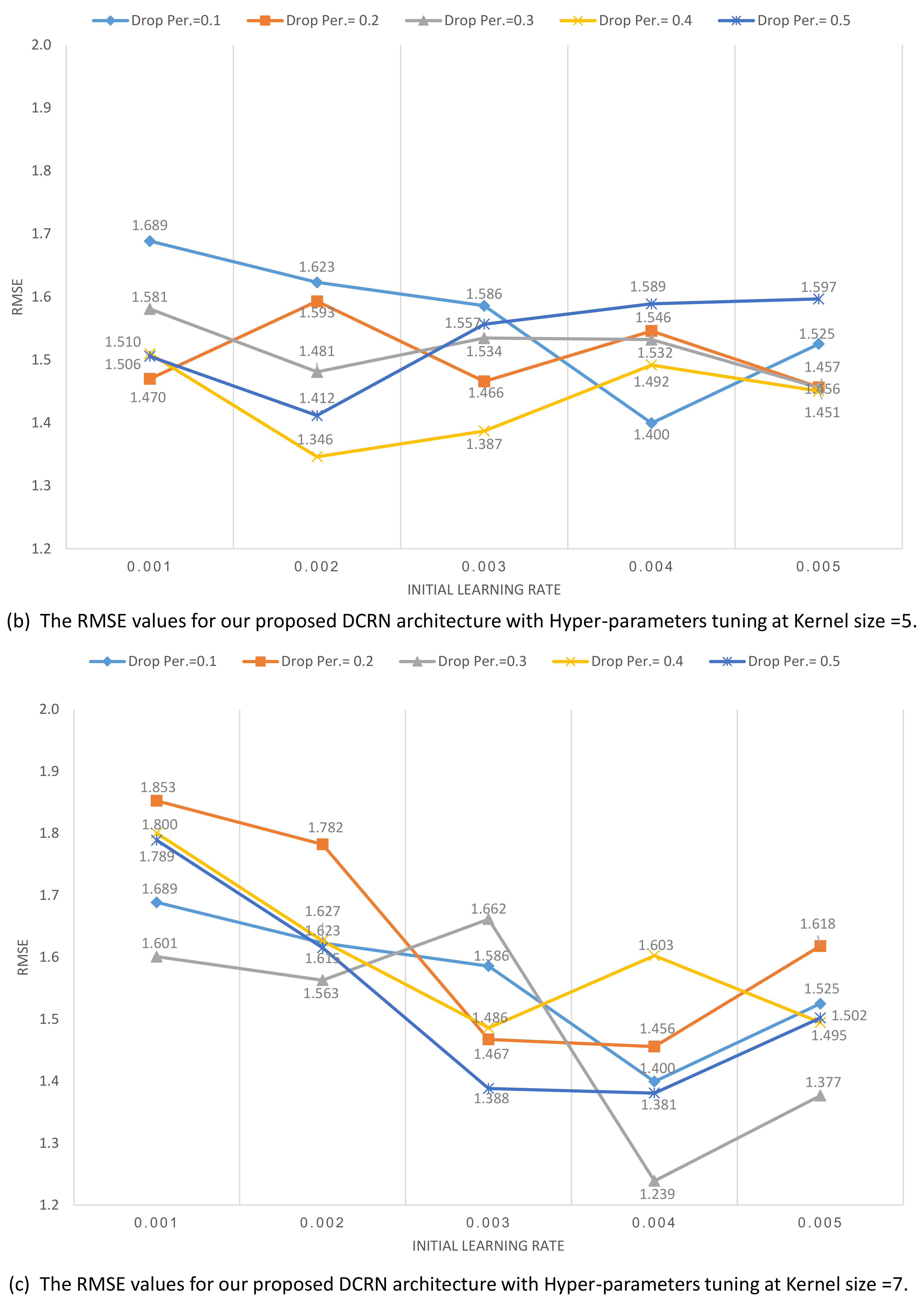
After investigating the DCRN depth layers and the best optimizer that working with it. We investigate the other hyper-parameters for DCRN architecture as shown in Figure 14. We investigate the dropout percentage, initial learning rate, and kernel sizes in each layer. The investigated hyper-parameters were examined as follows: dropout percentage (0.1, 0.2, 0.3, 0.4, 0.5), kernel size (3, 5, 7), and Initial learning rate (0.001, 0.002, 0.003, 0.004, 0.005). The results of hyper-parameters tuning of our proposed DCRN at kernel size = 3, 5, and 7 are shown in Figure 14a–c, respectively.

In this experiment, we have utilized the Experiment Manager tool in MATLAB 2020a which has generated 75 individual experiments. The lowest RMSE value (1.239) has been achieved with kernel size 7, initial learning rate 0.004, and drop percentage 0.3. Moreover, the optimized DCRN has achieved an Adjusted R-squared value of 0.99. The highest RMSE value (1.906) is achieved with kernel size 3 initial learning rate 0.002 and drop percentage 0.4.

In

Table 5. Our proposed approach building orientation angle estimation mean and SD values with building image contrast variation.

Building Orientation Angle	0	10	20	−10	−20
Mean	−0.03	10.2	19.9	−10.01	−20.61
SD	0.26	0.33	0.07	0.20	0.28

, we calculate the mean and the standard deviation (SD) values for the estimated angles results with the contrast variation of the input images. The estimation of buildings with orientation angle −10 has achieved the nearest mean value of 10.01 and the estimation of buildings with orientation angle 20 has achieved the lowest SD error. The estimation of buildings with orientation angle −20 has achieved a mean value of −20.61. On the contrary, the estimation of buildings with orientation angle +10 has achieved the largest SD value of 0.33.

4.5. Experiment 5

In this experiment, we compare our proposed optimized DCRN and the previous methods. The first method is based on morphological binary processing [42], the second method is based on Hough transform processing [3], and the remind methods are based on deep regression networks [46,49,59,60]. Firstly, to prove the generalization ability of our proposed approach, we visualize the building orientation angles mean ± variance values through all test set as shown in

Table 6. Our proposed building orientation angle estimation mean ± variance results vs. previous methods for all test set samples.

Building Orientation Angle	−10	−20	0	10	20	Mean Absolute Error
Morphological Processing [42]	−13.44 ± 1692.43	9.38 ± 2874.33	11.53 ± 1929.5	12.62 ± 2432.18	5.49 ± 8.61	12.29
Hough Transform [3]	−4.72 ± 912.73	−23.03 ± 323.72	−24.37 ± 327.85	−23.57 ± 288.56	−9.79 ± 7.88	19.21
Deep Learning Approach1 [46]	−9.65 ± 22.74	−16.57 ± 33.94	2.1 ± 11.59	7.27 ± 33.12	19.13 ± 27.47	1.90
Deep Learning Approach2 [59]	−10.12 ± 6.74	−18.51 ± 19.56	0.24 ± 2.5	8.58 ± 14.1	19.34 ± 9.23	0.79
Deep Learning Approach3 [49]	−9.91 ± 0.63	−19.7 ± 4.8	0.04 ± 0.23	9.81 ± 4.98	19.7 ± 1.03	0.18
Deep Learning Approach4 [60]	−9.39 ± 0.52	−19.47 ± 4.58	−0.01 ± 0.04	9.65 ± 4.17	19.35 ± 3.06	0.40
Our Optimized DCRN Approach	−10.03 ± 0.62	−19.8 ± 1.03	0.12 ± 0.37	9.58 ± 4.28	19.97 ± 1.01	0.16

. Secondly, we have selected random test samples with different building sizes, building designs, roof shapes, and roof colors to visualize our proposed approach robustness with buildings shape and color change.

The morphological processing approach has achieved its best performance when estimating angle −10 with a mean value of −13.44. However, the variance error has a value of 1692.43. The morphological processing approach has failed to estimate the building orientation angles 0, 20, and −20. The Hough transform approach has achieved its best performance when estimating angles −20 with a value of −23.03. However, the variance error of the estimation of angles −20 was high. The Hough transform approach has failed to estimate the orientation angles for angles 0, 10, and 20. The deep learning approach1 [46] has achieved its best performance during the estimation of buildings’ angles with a value of −10. However, the variance error was high at 22.74. It has achieved the worst results during the estimation of angle −20 with the highest variance value of 33.94. The deep learning approach2 [59] has achieved its best performance during the estimation of buildings’ angles with a value of −10. The deep learning approach3 [49] has achieved its best performance during the estimation of buildings’ angles with a value of 10. The deep learning approach4 [60] has achieved its best performance during the estimation of buildings’ angles with a value of 0. The deep learning approach4 has achieved the nearest mean value for estimating the building’s orientation angle 0. Our proposed approach has achieved the nearest mean values compared to the previous methods for estimating buildings with orientation angles −10, −20, and 20. For the estimation of angle −10, our optimized DCRN approach has achieved an average estimated value of −10.03 with a low variance error of 0.62. For the estimation of angle −20, our optimized DCRN approach has achieved an average estimated value of −19.8 with a low variance error of 1.03. For the estimation of angle 20, our optimized DCRN approach has achieved an average estimated value of 19.97 with a low variance error of 1.01. Finally, Our optimized DCRN approach has achieved the lowest mean absolute error for the angles’ means values with a value of 0.16.

For more explanation, we visualize ten different samples of building images as shown in

Table 7. Our proposed approach building orientation angle estimation results vs. previous methods.

No.	Image Sample	Correct Orientation Angle	Estimated Orientation Angle
			Morphological Processing [42]	Hough Transform [3]	Deep Learning Approach1 [46]	Deep Learning Approach2 [59]	Deep Learning Approach3 [49]	Deep Learning Approach4 [60]	Our Optimized DCRN Approach
1		0	87.51	−5.38	9.1	0.27	0.18	0.12	−0.11
2		0	−68.04	−4.6	0.02	9.06	0.3	0.32	−0.21
3		+10	−76.44	−22.4	4.97	9.36	10.5	9.9	10.05
4		+10	−60.05	23.71	5.4	7.65	9.69	9.8	9.84
5		−10	−12.42	−24.4	−13.52	−10.1	−10.2	−9.26	−9.93
6		−10	−27.98	−56.83	−13.12	−10.6	−10.4	−9.41	−10.23
7		−20	−67.34	14.4	−19.42	−20.9	−17.81	−19.8	−20.8
8		−20	−66.77	19.29	−23.48	−19.5	−19.49	−19.61	−19.68
9		+20	−2.3	64	20.22	19.49	19.9	19.5	20.56
10		+20	83.69	40	16.99	20.09	19.92	19.94	19.99

. The second column represents the original image sample, the third column represents the correct orientation angle of the building sample, the fourth column represents the estimated orientation angle based on morphological processing approach, the fifth column represents the estimated orientation angle based on the Hough transform processing approach, from sixth to ninth columns represent the estimated orientation angles based on the previous deep learning networks. Finally, the last column represents the estimated orientation angles based on our optimized DCRN approach.

4.6. Experiment 6

In this experiment, we perform a computational cost analysis for our proposed approach vs. the previous methods at two levels. In the first level, all methods are compared based on training and inference processes. We compare our proposed DCRN approach vs. the previous deep learning approaches, as shown in

Table 8. Our proposed DCRN approach for building orientation angle estimation processing time results vs. the previous deep learning methods.

	Deep Learning Approach1 [46]	Deep Learning Approach2 [59]	Deep Learning Approach3 [49]	Deep Learning Approach4 [60]	Our Optimized DCRN Approach
Training Time (min)	31	20	248	38	19
Inference Time (s)	0.02	0.01	0.03	0.02	0.01
Training/Inference	9.30 × 10${}^{+04}$	1.20 × 10${}^{+05}$	5.72 × 10${}^{+05}$	1.14 × 10${}^{+05}$	1.14 × 10${}^{+05}$

. In the second level, all methods are compared based on inference process only. we compare our proposed DCRN approach and the other buildings’ angle orientation estimation techniques based on traditional image processing, as shown in

Table 9. Our proposed DCRN approach for building orientation angle estimation processing time results vs.the previous traditional image processing methods.

	Processing Time (Mean ± Var) (s)
Morphological Processing [42]	0.29 ± 0.08
Hough Transform [3]	0.56 ± 0.17
Our Optimized DCRN	0.01 ± 0.014

.

Our proposed DCRN approach has achieved the lowest training time, with 19 min. On the other hand, the deep learning approach2 has achieved the second rank for training time with 20 min. The deep learning approach1 has achieved the third rank of the training time with 31 min. The deep learning approach4 has achieved a high training time of 38 min. The deep learning approach3 has achieved the highest training time with 248 min. Our proposed DCRN and the deep learning approach2 have achieved the lowest inference time with 0.01 s. Our proposed DCRN approach and deep learning approach2 have achieved the lowest inference time with a value of 0.01 s. The deep learning approach3 has achieved the highest inference time with a value of 0.03 s. Our proposed DCRN approach has achieved a low training/inference ratio with a value of 1.14 × ${10}^5$. The deep learning approach4 has achieved a similar training/inference ratio similar to our proposed DCRN approach. The deep learning approach1 has achieved the lowest training/inference ratio with a value of 9.3 × ${10}^4$.

As shown in Table 9, our proposed DCRN approach has achieved the highest performance of mean value 0.01 s of the processing inference time. The Morphological processing approach has achieved the mean value of 0.29 s of the processing inference time with the least variance value. The Hough transform approach has achieved the highest mean value of 0.56 s of the processing inference time.

4.7. Experiment 7

In this experiment, we try to answer the question of “how is the decision-making in each algorithm?” Each algorithm follows some procedures to get the ordination angle of the building. We visualize ten different samples of building images as shown in

Table 10. The deep activation kernels of our proposed approach vs. traditional methods.

No.	Image Sample	Morphological Processing [42]	Hough Transform [3]	Our Optimized DCRN
1
2
3
4
5
6
7
8
9
10

. The second column represents the original image sample, the third column represents the morphological processing approach, the third column represents the Hough transform processing approach, and the last column represents our proposed DCRN approach. In each algorithm, the estimated orientation angle is calculated by different methodologies. In the morphological approach, the angle is detected through the biggest binary blob in the image. In the Hough transform approach, the angle is detected through the average orientation angles of lines detected on the corners. In our proposed approach, the angle is detected through the convolutional filters, which are applied to the input images. Then, the filters construct their learnable parameters through the training process. In our proposed DCRN approach, we visualize the strongest activation kernel. As the complexity of building roof appearance, the unsupervised approaches reflects the low performance of estimated orientation angle. However, CNN features in most of the images reflect the main edges of the building, which reflect on the effectiveness of orientation angle estimation.

5. Discussion

In experiment 1, the plain networks have demonstrated a low performance. Furthermore, the VGGNet architecture failed to estimate building orientation angle after fine-tuning. AlexNet has achieved a high RMSE value with both utilized optimizers. Inception GoogleNet architecture has achieved a better performance than plain networks. Moreover, GoogleNet has achieved a lower RMSE value than ResNet18 architecture with ADAM optimizer. However, ResNet18 architecture has achieved a lower RMSE value than GoogleNet architecture. Both of EffiicentNet and ResNet18 have achieved a similar RMSE value with the RMS optimizer. We have concluded that the RMS optimizer has increased the effectiveness of deep plain networks such as AlexNet, VGG16, and VGG19. Besides that, the RMS optimizer has also increased the performance of ResNet101 architecture. Moreover, the ADAM optimizer has enhanced the performance of GoogleNet, ResNet18, ResNet50, MobileNetv2, and EfficientNet. We have concluded that the transfer-learning approach from image classification task to image regression task has some limitations in its accuracy and consumes long training time. The need to highly upsampling of the input image size to fit the pre-trained networks may decrease the estimation accuracy. The boundary of the buildings which visually detect each building orientation angle has low contrast in color images which makes a real need to increase the buildings’ boundary using image processing sharpening techniques.

In experiment 2, the proposed DCRN architecture with depth c has achieved the highest performance with the RMS optimizer. This means that increasing the network depth increased the overall system performance. We have concluded that DCRN architecture C has achieved the best performance that confirmed that the increase of DCRN architecture depth has increased the proposed model performance. However, DCRN with depth A and depth B has achieved a lower accuracy than architecture with depth C. On the other hand, our proposed DCRN architecture has achieved the lowest performance with depth A. In our proposed DCRN, the RMS optimizer has worked better with different DCRN depths. We have found that our proposed DCRN approach achieved lower RMS value than transfer-learning approach. From experiment 2, it is demonstrated that training a deep regression network from scratch is better than pre-trained networks fine-tuning. The color information for building orientation angle estimation is not useful. The low image input layer for the deep network as in our proposed DCRN network has performed better than the high size image input layer in the pre-trained networks.

In experiment3, our proposed SG layer has enhanced the performance of DCRN architecture as expected from experiments 1 and 2. The proposed gradient layer has solved the shadows, poor building edges appearance, and low contrast problems. Moreover, the SG layer has worked better with the RMS optimizer and has achieved the highest performance. We have found that the RMS optimizer during training and validation phases has highly oscillated more than ADAM optimizer. However, it achieved a 1.8 RMSE value lower than the ADAM optimizer in the existence of the SG layer. Both evaluation metrics RMSE and Adjusted R-squared values have proven the superior performance of the RMS optimizer with our estimation task. The gradient layer was very efficient and help the deep network to extract more discriminated features.

In experiment 4, we have performed the hyper-parameters tuning for our proposed DCRN architecture to achieve the best performance. The lowest RMSE values have been achieved with the high kernel size (7), the second rank of the lowest RMSE value has been achieved with kernel size (5). Experiment 4 has demonstrated that the small kernel size has increased the RMSE value for our proposed DCRN architecture and has decreased its performance. Furthermore, the lowest RMSE value has been achieved with the high initial learning rate (0.004), the second rank of the lowest RMSE value has been achieved with the initial learning rate (0.003). Experiment 4 has demonstrated that the low learning initial rate value has increased the RMSE value for our proposed DCRN architecture and consequently has decreased its performance. Finally, the lowest RMSE value has been achieved with the low drop percentage (0.3), the second rank of the lowest RMSE value has achieved with drop percentage (0.1). Furthermore, the high drop percentage value has increased the RMSE value for our proposed DCRN architecture and has decreased its performance. We have concluded that the hyper-parameters tuning plays a crucial role in our proposed DCRN network performance. The residual plots error variation through the estimated angles reflect the low performance during the estimation of −20 angle. However, the error variation in all other angles is accepted. This provides an additional evidence for the superior capabilities of deep regression networks to extract building characteristics from high-resolution satellite images. We have proved the robustness of our proposed approach with the variation of building image contrast. We have noticed the stability of our building orientation angle estimation approach with different contrast conditions. We have noticed that each building orientation angle estimation has been varied individually with the contrast variation.

In experiment 5, we compare our proposed approach and the traditional image processing techniques and the other deep learning techniques. The results showed that the high superiority of our proposed DCRN architecture compared with the previous methods. The morphological-based approach lacked robustness and achieved the highest error values. This bad performance of traditional morphological binary processing refers to the sensitivity of the algorithm to the details inside the building roof, the design of the building, and the shadows effect. Furthermore, Hough transform-based approach has achieved better performance than the morphological processing approach in some of the angles estimation results. However, the Hough lines are very sensitive to non-real corners of the building because of the variation of roof design. In some samples, the two previous approaches failed to estimate the direction of orientation angles. The deep learning approach1 based on VGG16 and the deep learning approach2 based on AlexNet have achieved the worst estimation results among the other deep learning approaches. The deep learning approach3 based on ResNet101 architecture and the deep learning approach4 based on Xception architecture have achieved better results than VGG16 and AlexNet Architectures. On the other hand, our optimized DCRN approach has achieved the best results in most samples. Our proposed approaches have achieved the lowest error values. The deep learning approach presented in [46] was embedded with the detection task. This proves that a separated network for object orientation detection is better than the embedded one [46]. Our optimized DCRN approach reflects its super-capability in the estimation of building orientation angle with the minimum error values from different angles after hyper-parameters optimization.

In experiment 6, we have performed a computational cost analysis for our proposed approach and the other approaches in the literature. The findings clearly has indicated that the plain networks have achieved the lowest training time, inference time, and training/inference ratio. Furthermore, our proposed DCRN architecture has achieved the lowest training and inference time. The deep learning approach2 based on AlexNet architecture has a similar inference time as our proposed DCRN approach. However, the deep learning approach4 based on Xception architecture has the same training/inference ratio as our proposed DCRN approach. Our Proposed DCRN architecture has achieved a lower processing time than the Hough transform-based and morphological-based approaches. The morphological-based approach has achieved the highest error values with a high variance of processing time. However, our proposed DCRN has achieved the lowest error values with the lowest variance of the processing time.

In experiment 7, we visualize the CNN features aiming to ensure the effectiveness of our proposed DCRN architecture. The visualization of the previous methods has ensured that the problems found in these methods required more processes, which increased the algorithm’s complexity. The building’s roof shapes are very complex, and finding the edges of such shapes is very difficult. Furthermore, sharped corners and the variations in building roof design generated corners, which confused the Hough transform algorithm. However, the visualized activated kernels of the highest kernels show that the correct edges of the building with correct orientation angles were detected.

6. Conclusions

In this paper, we propose two different approaches for building orientation estimation. The first approach is based on the transfer learning approach. The lowest RMSE value (2.2) based on transfer-learning of MobileNetV2 architecture has been achieved with the ADAM optimizer. The second approach based on our proposed DCRN architecture has achieved an RMSE value of 2.4. Besides that, the SG layer has achieved an RMSE value of 1.8. The optimized DCRN network has achieved better performance with the lowest RMSE value 1.2. The comparison of our proposed approaches vs. previous methods reflects the high performance of our solution for estimating the building orientation angle. An explanation based on CNN features visualization is also provided for our DCRN architecture. The visualized kernels reflect the correct edges in the estimation of the building orientation angle. The optimizer plays a critical role to enhance the deep network performance. RMS optimizer has achieved a lower RMSE value than ADAM optimizer. The cost processing time of our approach is reasonable and achieved the lowest variance error. Experiments have been carried on 15,190 building images with different designs, shapes, angles, and lighting conditions. These experiments have verified the effectiveness of our proposed approach. We proved that building characteristics could be estimated through high-resolution satellite images. For future works, other building characteristics would be estimated, there is still a challenge to decrease the RMSE value of the estimated orientation angle, and the processing time can be decreased through decreasing network complexity. Several modifications to the DCRN network architecture can increase its performance such as residual and inception units. The loss function modification can play a crucial role to increase the estimation performance and decrease the error. The hyper-parameters tuning can be accelerated and the hyper-parameters optimization of the DCRN network can increase the DCRN network performance.

References

1. Coutts, A.M.; Harris, R.J.; Phan, T.; Livesley, S.J.; Williams, N.S.; Tapper, N.J. Thermal infrared remote sensing of urban heat: Hotspots, vegetation, and an assessment of techniques for use in urban planning. Remote Sens. Environ. 2016, 186, 637–651. [Google Scholar] [CrossRef]
2. Kadhim, N.; Mourshed, M.; Bray, M. Advances in remote sensing applications for urban sustainability. Euro-Mediterr. J. Environ. Integr. 2016, 1, 7. [Google Scholar] [CrossRef] [Green Version]
3. Wang, R.; Hu, Y.; Wu, H.; Wang, J. Automatic extraction of building boundaries using aerial LiDAR data. J. Appl. Remote Sens. 2016, 10, 016022. [Google Scholar] [CrossRef]
4. Zeng, Y.; Huang, W.; Liu, M.; Zhang, H.; Zou, B. Fusion of satellite images in urban area: Assessing the quality of resulting images. In Proceedings of the 2010 18th International Conference on Geoinformatics, Beijing, China, 18–20 June 2010; pp. 1–4. [Google Scholar]
5. Quinn, J.A.; Nyhan, M.M.; Navarro, C.; Coluccia, D.; Bromley, L.; Luengo-Oroz, M. Humanitarian applications of machine learning with remote-sensing data: Review and case study in refugee settlement mapping. Philos. Trans. R. Soc. A Math. Phys. Eng. Sci. 2018, 376, 20170363. [Google Scholar] [CrossRef] [Green Version]
6. Hau, C.C. Handbook of Pattern Recognition and Computer Vision; World Scientific: Singapore, 2015. [Google Scholar]
7. Dey, V.; Zhang, Y.; Zhong, M. A review on image segmentation techniques with remote sensing perspective. In Proceedings of the ISPRS TC VII Symposium—100 Years ISPRS, Vienna, Austria, 5–7 July 2010; Volume 38. [Google Scholar]
8. Zhang, X.; Ai, T.; Stoter, J.; Kraak, M.J.; Molenaar, M. Building pattern recognition in topographic data: Examples on collinear and curvilinear alignments. Geoinformatica 2013, 17, 1–33. [Google Scholar] [CrossRef] [Green Version]
9. Ball, J.; Anderson, D.; Chan, C.S. Comprehensive survey of deep learning in remote sensing: Theories, tools, and challenges for the community. J. Appl. Remote Sens. 2017, 11, 042609. [Google Scholar] [CrossRef] [Green Version]
10. LeCun, Y.; Bottou, L.; Bengio, Y.; Haffner, P. Gradient-based learning applied to document recognition. Proc. IEEE 1998, 86, 2278–2324. [Google Scholar] [CrossRef] [Green Version]
11. Liang, H.; Sun, X.; Sun, Y.; Gao, Y. Text feature extraction based on deep learning: A review. EURASIP J. Wirel. Commun. Netw. 2017, 2017, 1–12. [Google Scholar] [CrossRef]
12. Kim, J.R.; Shim, W.H.; Yoon, H.M.; Hong, S.H.; Lee, J.S.; Cho, Y.A.; Kim, S. Computerized bone age estimation using deep learning based program: Evaluation of the accuracy and efficiency. Am. J. Roentgenol. 2017, 209, 1374–1380. [Google Scholar] [CrossRef]
13. Lore, K.G.; Akintayo, A.; Sarkar, S. LLNet: A deep autoencoder approach to natural low-light image enhancement. Pattern Recognit. 2017, 61, 650–662. [Google Scholar] [CrossRef] [Green Version]
14. Kemker, R.; Salvaggio, C.; Kanan, C. Algorithms for semantic segmentation of multispectral remote sensing imagery using deep learning. ISPRS J. Photogramm. Remote Sens. 2018, 145, 60–77. [Google Scholar] [CrossRef] [Green Version]
15. Ma, L.; Liu, Y.; Zhang, X.; Ye, Y.; Yin, G.; Johnson, B.A. Deep learning in remote sensing applications: A meta-analysis and review. ISPRS J. Photogramm. Remote Sens. 2019, 152, 166–177. [Google Scholar] [CrossRef]
16. Li, M.; Zang, S.; Zhang, B.; Li, S.; Wu, C. A review of remote sensing image classification techniques: The role of spatio-contextual information. Eur. J. Remote Sens. 2014, 47, 389–411. [Google Scholar] [CrossRef]
17. Zhu, X.X.; Tuia, D.; Mou, L.; Xia, G.S.; Zhang, L.; Xu, F.; Fraundorfer, F. Deep learning in remote sensing: A comprehensive review and list of resources. IEEE Geosci. Remote Sens. Mag. 2017, 5, 8–36. [Google Scholar] [CrossRef] [Green Version]
18. Zhang, Y. Optimisation of building detection in satellite images by combining multispectral classification and texture filtering. ISPRS J. Photogramm. Remote Sens. 1999, 54, 50–60. [Google Scholar] [CrossRef]
19. Yang, X.; Sun, H.; Fu, K.; Yang, J.; Sun, X.; Yan, M.; Guo, Z. Automatic ship detection in remote sensing images from google earth of complex scenes based on multiscale rotation dense feature pyramid networks. Remote Sens. 2018, 10, 132. [Google Scholar] [CrossRef] [Green Version]
20. Ji, H.; Gao, Z.; Mei, T.; Ramesh, B. Vehicle detection in remote sensing images leveraging on simultaneous super-resolution. IEEE Geosci. Remote Sens. Lett. 2019, 17, 676–680. [Google Scholar] [CrossRef]
21. Bégué, A.; Arvor, D.; Bellon, B.; Betbeder, J.; De Abelleyra, D.; PD Ferraz, R.; Lebourgeois, V.; Lelong, C.; Simões, M.; Verón, S.R. Remote sensing and cropping practices: A review. Remote Sens. 2018, 10, 99. [Google Scholar] [CrossRef] [Green Version]
22. Bolanos, S.; Stiff, D.; Brisco, B.; Pietroniro, A. Operational surface water detection and monitoring using Radarsat 2. Remote Sens. 2016, 8, 285. [Google Scholar] [CrossRef] [Green Version]
23. Hatamizadeh, A.; Sengupta, D.; Terzopoulos, D. End-to-end trainable deep active contour models for automated image segmentation: Delineating buildings in aerial imagery. In Proceedings of the European Conference on Computer Vision, Glasgow, UK, 23–28 August 2020; pp. 730–746. [Google Scholar]
24. Sun, S.; Mu, L.; Wang, L.; Liu, P.; Liu, X.; Zhang, Y. Semantic Segmentation for Buildings of Large Intra-Class Variation in Remote Sensing Images with O-GAN. Remote Sens. 2021, 13, 475. [Google Scholar] [CrossRef]
25. Yi, Y.; Zhang, Z.; Zhang, W.; Zhang, C.; Li, W.; Zhao, T. Semantic segmentation of urban buildings from VHR remote sensing imagery using a deep convolutional neural network. Remote Sens. 2019, 11, 1774. [Google Scholar] [CrossRef] [Green Version]
26. Liu, J.; Wang, S.; Hou, X.; Song, W. A deep residual learning serial segmentation network for extracting buildings from remote sensing imagery. Int. J. Remote Sens. 2020, 41, 5573–5587. [Google Scholar] [CrossRef]
27. Abdollahi, A.; Pradhan, B.; Alamri, A.M. An ensemble architecture of deep convolutional Segnet and Unet networks for building semantic segmentation from high-resolution aerial images. Geocarto Int. 2020, 1–16. [Google Scholar] [CrossRef]
28. Wang, C.; Li, L. Multi-Scale Residual Deep Network for Semantic Segmentation of Buildings with Regularizer of Shape Representation. Remote Sens. 2020, 12, 2932. [Google Scholar] [CrossRef]
29. Shahin, A.I.; Almotairi, S. SVA-SSD: Saliency visual attention single shot detector for building detection in low contrast high-resolution satellite images. PeerJ Comput. Sci. 2021, 7, e772. [Google Scholar] [CrossRef]
30. Li, Y.; Hu, W.; Dong, H.; Zhang, X. Building damage detection from post-event aerial imagery using single shot multibox detector. Appl. Sci. 2019, 9, 1128. [Google Scholar] [CrossRef] [Green Version]
31. Zhang, L.; Wu, J.; Fan, Y.; Gao, H.; Shao, Y. An Efficient Building Extraction Method from High Spatial Resolution Remote Sensing Images Based on Improved Mask R-CNN. Sensors 2020, 20, 1465. [Google Scholar] [CrossRef] [PubMed] [Green Version]
32. Ma, H.; Liu, Y.; Ren, Y.; Yu, J. Detection of Collapsed Buildings in Post-Earthquake Remote Sensing Images Based on the Improved YOLOv3. Remote Sens. 2020, 12, 44. [Google Scholar] [CrossRef] [Green Version]
33. Liasis, G.; Stavrou, S. Satellite images analysis for shadow detection and building height estimation. ISPRS J. Photogramm. Remote Sens. 2016, 119, 437–450. [Google Scholar] [CrossRef]
34. Nemoto, K.; Hamaguchi, R.; Sato, M.; Fujita, A.; Imaizumi, T.; Hikosaka, S. Building change detection via a combination of CNNs using only RGB aerial imageries. Remote Sens. Technol. Appl. Urban Environ. II 2017, 10431, 104310J. [Google Scholar]
35. More, N.; Singh, R.; Murugan, G. Automatic Building Roof Detection Using Novel Image Morphology Operations. In Proceedings of the 2nd International Conference on Advances in Science & Technology (ICAST), Bahir Dar, Ethiopia, 2–4 August 2019. [Google Scholar]
36. Karatsiolis, S.; Kamilaris, A.; Cole, I. IMG2nDSM: Height Estimation from Single Airborne RGB Images with Deep Learning. Remote Sens. 2021, 13, 2417. [Google Scholar] [CrossRef]
37. Li, X.; Wang, M.; Fang, Y. Height estimation from single aerial images using a deep ordinal regression network. IEEE Geosci. Remote Sens. Lett. 2020. [Google Scholar] [CrossRef]
38. Liu, C.J.; Krylov, V.A.; Kane, P.; Kavanagh, G.; Dahyot, R. IM2ELEVATION: Building Height Estimation from Single-View Aerial Imagery. Remote Sens. 2020, 12, 2719. [Google Scholar] [CrossRef]
39. Cao, Y.; Huang, X. A deep learning method for building height estimation using high-resolution multi-view imagery over urban areas: A case study of 42 Chinese cities. Remote Sens. Environ. 2021, 264, 112590. [Google Scholar] [CrossRef]
40. Sun, J.; Zhou, W.; Li, H. Orientation estimation network. In Proceedings of the International Conference on Image and Graphics, Shanghai, China, 13–15 September 2017; pp. 151–162. [Google Scholar]
41. Amini, H.; Arefi, H. CNN-based estimation of pre-and post-earthquake height models from single optical images for identification of collapsed buildings. Remote Sens. Lett. 2019, 10, 679–688. [Google Scholar] [CrossRef]
42. Ghandour, A.J.; Jezzini, A.A. Autonomous building detection using edge properties and image color invariants. Buildings 2018, 8, 65. [Google Scholar] [CrossRef] [Green Version]
43. Nguyen, T.H.; Daniel, S.; Gueriot, D.; Sintes, C.; Caillec, J.M.L. Unsupervised Automatic Building Extraction Using Active Contour Model on Unregistered Optical Imagery and Airborne LiDAR Data. arXiv 2019, arXiv:1907.06206. [Google Scholar] [CrossRef] [Green Version]
44. Bachiller-Burgos, P.; Manso, L.J.; Bustos, P. A variant of the Hough Transform for the combined detection of corners, segments, and polylines. EURASIP J. Image Video Process. 2017, 2017, 32. [Google Scholar] [CrossRef] [Green Version]
45. Kadhim, N.; Mourshed, M. A shadow-overlapping algorithm for estimating building heights from VHR satellite images. IEEE Geosci. Remote Sens. Lett. 2017, 15, 8–12. [Google Scholar] [CrossRef] [Green Version]
46. Chen, Y.; Gong, W.; Chen, C.; Li, W. Learning orientation-estimation convolutional neural network for building detection in optical remote sensing image. In Proceedings of the 2018 Digital Image Computing: Techniques and Applications (DICTA), Canberra, Australia, 10–13 December 2018; pp. 1–8. [Google Scholar]
47. Wang, J.; Lu, C.; Jiang, W. Simultaneous ship detection and orientation estimation in SAR images based on attention module and angle regression. Sensors 2018, 18, 2851. [Google Scholar] [CrossRef] [Green Version]
48. Tang, T.; Zhou, S.; Deng, Z.; Lei, L.; Zou, H. Arbitrary-oriented vehicle detection in aerial imagery with single convolutional neural networks. Remote Sens. 2017, 9, 1170. [Google Scholar] [CrossRef] [Green Version]
49. Hara, K.; Vemulapalli, R.; Chellappa, R. Designing deep convolutional neural networks for continuous object orientation estimation. arXiv 2017, arXiv:1702.01499. [Google Scholar]
50. Phisannupawong, T.; Kamsing, P.; Torteeka, P.; Channumsin, S.; Sawangwit, U.; Hematulin, W.; Jarawan, T.; Somjit, T.; Yooyen, S.; Delahaye, D.; et al. Vision-based spacecraft pose estimation via a deep convolutional neural network for noncooperative docking operations. Aerospace 2020, 7, 126. [Google Scholar] [CrossRef]
51. Li, H.; Li, Q.; Wu, G.; Chen, J.; Liang, S. The impacts of building orientation on polarimetric orientation angle estimation and model-based decomposition for multilook polarimetric SAR data in Urban areas. IEEE Trans. Geosci. Remote Sens. 2016, 54, 5520–5532. [Google Scholar] [CrossRef]
52. Maslikowski, L.; Samczynski, P.; Baczyk, M.; Krysik, P.; Kulpa, K. Passive bistatic SAR imaging—Challenges and limitations. IEEE Aerosp. Electron. Syst. Mag. 2014, 29, 23–29. [Google Scholar] [CrossRef]
53. Kandel, I.; Castelli, M. How Deeply to Fine-Tune a Convolutional Neural Network: A Case Study Using a Histopathology Dataset. Appl. Sci. 2020, 10, 3359. [Google Scholar] [CrossRef]
54. Deng, J.; Dong, W.; Socher, R.; Li, L.J.; Li, K.; Fei-Fei, L. Imagenet: A large-scale hierarchical image database. In Proceedings of the 2009 IEEE Conference on Computer Vision and Pattern Recognition, Miami, FL, USA, 20–25 June 2009; pp. 248–255. [Google Scholar]
55. Chen, F.; Wang, N.; Yu, B.; Qin, Y.; Wang, L. A Strategy of Parallel Seed-Based Image Segmentation Algorithms for Handling Massive Image Tiles over the Spark Platform. Remote Sens. 2021, 13, 1969. [Google Scholar] [CrossRef]
56. Yang, X.; Sun, H.; Sun, X.; Yan, M.; Guo, Z.; Fu, K. Position detection and direction prediction for arbitrary-oriented ships via multitask rotation region convolutional neural network. IEEE Access 2018, 6, 50839–50849. [Google Scholar] [CrossRef]
57. Sameen, M.I.; Pradhan, B.; Aziz, O.S. Classification of very high resolution aerial photos using spectral-spatial convolutional neural networks. J. Sensors 2018, 2018, 7195432. [Google Scholar] [CrossRef] [Green Version]
58. Hutter, F.; Lücke, J.; Schmidt-Thieme, L. Beyond manual tuning of hyperparameters. KI Künstliche Intell. 2015, 29, 329–337. [Google Scholar] [CrossRef]
59. Fischer, P.; Dosovitskiy, A.; Brox, T. Image orientation estimation with convolutional networks. In Proceedings of the German Conference on Pattern Recognition, Aachen, Germany, 7–10 October 2015; pp. 368–378. [Google Scholar]
60. Lucas, J.; Kyono, T.; Werth, M.; Gagnier, N.; Endsley, Z.; Fletcher, J.; McQuaid, I. Estimating Satellite Orientation through Turbulence with Deep Learning. In Proceedings of the Advanced Maui Optical and Space Surveillance Technologies Conference (AMOS), Marriott Maui, Maui, HI, USA, 15–18 September 2020. [Google Scholar]
Figure 1. (a) High-resolution satellite image shows different building orientation angles in dense building view in Riyadh city, (b) linear building alignment representation, (c) curvilinear building alignment representation, and (d) grid building alignment representation with different orientation angles.
Electronics 10 02970 g001
Figure 2. A sample of building images with different orientation angles from our collected dataset from Riyadh city (a) building image with orientation angle 0, (b) building image with orientation angle +10, (c) building image with orientation angle −10, (d) building image with orientation angle −20, and (e) building image with orientation angle +20.
Electronics 10 02970 g002
Figure 3. The first proposed approach based on transfer learning for building orientation angle estimation.
Electronics 10 02970 g003
Figure 4. The second proposed approach based on DCRN for building angle orientation estimation.
Electronics 10 02970 g004
Figure 5. A sample for building image enhancement using SG layer: (a) Before SG layer; (b) After SG layer.
Electronics 10 02970 g005
Figure 6. The proposed DCRN with three architectures (a) depth A, (b) depth B, and (c) depth C.
Electronics 10 02970 g006
Figure 7. The achieved RMSE values with our proposed DCRN with three architectures depths A, B, and C.
Electronics 10 02970 g007
Figure 8. The proposed DCRN training loss function performance with SG layer based different optimizers.
Electronics 10 02970 g008
Figure 9. The proposed DCRN training RMSE performance with SG layer based different optimizers.
Electronics 10 02970 g009
Figure 10. The proposed DCRN validation loss performance with SG layer based different optimizers.
Electronics 10 02970 g010
Figure 11. The proposed DCRN validation RMSE performance with SG layer based different optimizers.
Electronics 10 02970 g011
Figure 12. The residual variation in building orientation angle estimation based on Boxplots diagram.
Electronics 10 02970 g012
Figure 13. The effect of building image contrast variation on the building orientation estimation results for our proposed approach.
Electronics 10 02970 g013
Figure 14. The RMSE values for our proposed DCRN architecture with Hyper-parameters tuning.
Electronics 10 02970 g014aElectronics 10 02970 g014b