Article

Effective Voting Ensemble of Homogenous Ensembling with Multiple Attribute-Selection Approaches for Improved Identification of Thyroid Disorder

1
School of Mechanical and Manufacturing Engineering, National University of Sciences and Technology, Islamabad 44000, Pakistan
2
Department of Electrical Engineering, Riphah International University, Islamabad 44000, Pakistan
3
Department of Electrical and Computer Engineering, Faculty of Engineering and Applied Science, Memorial University of Newfoundland, St. John’s, NL A1B 3X5, Canada
4
National Centre of Artificial Intelligence (NCAI), Islamabad 44000, Pakistan
*
Author to whom correspondence should be addressed.
Submission received: 9 November 2021 / Revised: 27 November 2021 / Accepted: 30 November 2021 / Published: 3 December 2021

Abstract

:
Thyroid disease is characterized by abnormal development of glandular tissue on the periphery of the thyroid gland. Thyroid disease occurs when this gland produces an abnormally high or low level of hormones, with hyperthyroidism (active thyroid gland) and hypothyroidism (inactive thyroid gland) being the two most common types. The purpose of this work was to create an efficient homogeneous ensemble of ensembles in conjunction with numerous feature-selection methodologies for the improved detection of thyroid disorder. The dataset employed is based on real-time thyroid information obtained from the District Head Quarter (DHQ) teaching hospital, Dera Ghazi (DG) Khan, Pakistan. Following the necessary preprocessing steps, three types of attribute-selection strategies; Select From Model (SFM), Select K-Best (SKB), and Recursive Feature Elimination (RFE) were used. Decision Tree (DT), Gradient Boosting (GB), Logistic Regression (LR), and Random Forest (RF) classifiers were used as promising feature estimators. The homogeneous ensembling activated the bagging- and boosting-based classifiers, which were then classified by the Voting ensemble using both soft and hard voting. Accuracy, sensitivity, mean square error, hamming loss, and other performance assessment metrics have been adopted. The experimental results indicate the optimum applicability of the proposed strategy for improved thyroid ailment identification. All of the employed approaches achieved 100% accuracy with a small feature set. In terms of accuracy and computational cost, the presented findings outperformed similar benchmark models in its domain.

1. Introduction

The thyroid gland is located near the base of the neck and is responsible for secreting thyroid hormones, which play an important role in human metabolism [1]. When this gland is active, it secretes an excessive amount of hormone, which is referred to as hyperthyroidism. In contrast, insufficient thyroid hormone secretion results in hypothyroidism. The thyroid gland creates the thyroid hormones levothyroxine also known as T4 and triiodothyronine, also referred to as T3 in [2,3].
Hyperthyroidism is characterized by an abnormally high level of secretion. The human body’s metabolism is quick, and a person may have symptoms such as rapid weight loss, irregular heartbeat, high blood pressure, and so on [4,5]. On the contrary, hypothyroidism is caused by a lack of hormone secretion, which may cause a person to experience sluggishness in metabolism, abrupt weight gain, slow heartbeat with a low pulse rate. Another very common sign is low blood pressure. All these are the main symptoms of hypothyroidism [6,7]. For early prediction and diagnosis of thyroid disease, a blood test is usually performed by most medical experts. T4, T3, and TSH hormone levels are measured [8]. It is very important and the need of the hour to raise public awareness related to the symptoms, kinds, and diagnostic methods of this disease. Thyroid function testing is the most commonly used diagnostic test in the endocrine system. It is used as a screening tool to confirm the proper diagnosis of hyperthyroidism and hypothyroidism, to evaluate the effectiveness of medicinal treatment, and to monitor patients with differentiated thyroid cancer [9]. However, these methods are complex, time taking, and have low diagnosis efficiency, with soreness and bruising effects on the human body [10].
In the last few years, artificial intelligence has been widely used in various aspects for the better classification of thyroid disease. Aside from clinical examination, machine learning (ML) algorithms have been used effectively to achieve proper interpretation of thyroid data and early diagnosis of thyroid illness. Several studies have been conducted to determine the efficacy of these approaches. For example, Singh in [11] used thyroid nodule ultrasound images to apply the K-nearest neighbors (KNN), support vector machines (SVM), and Bayesian classification. Erol et al. [12] used a multilayer perceptron and radial basis function neural (MLPRBFN) network to classify thyroid disease structurally. Aside from these research findings, there are others (stated in Section 1.2) that use a wide range of learning methodologies to discover some significant insights about thyroid illness.
The goal of this study was to develop an efficient, homogeneous ensemble of ensembles that could be utilized, in conjunction with some attribute-selection strategies, to improve thyroid illness detection. Two thyroid datasets were examined in this study. After completing the necessary preprocessing stages, the Select From Model (SFM), Recursive Feature Elimination (RFE), and Select K-best (SKB) feature-selection techniques were deployed. The Logistic Regression (LR), Random Forest (RF), Decision Trees (DT), and Gradient Boosting (GB) were used for attribute estimation. The homogeneous ensemble was used to activate the bagging- and boosting-based classifiers, which were then further graded by voting ensemble (soft and hard) voting. Accuracy, mean square error (MSE), hamming loss, and various other performance evaluation measures have been implemented. This is the order in which the rest of the manuscript is structured: classification of thyroid disease by using ML methodologies is discussed in detail in Section 1, which includes a review of the relevant literature. Section 2 illustrates how the tests will be carried out according to the planned process or methodology. A detailed description of the used datasets is also included in this part. Section 3 summarizes the findings and results with discussions. Lastly, concluding notes are included in the final section to wrap off this research.

1.1. Research Contribution

Aside from the clinical and necessary examination, correct interpretation of thyroid illness is also necessary for better diagnosis. Therefore, this work contributed the following findings for the efficient and effective treatment of thyroid disorder.
  • Researchers achieved a lot of success in detecting thyroid illnesses, however, it is advised to utilize several parameters to diagnose thyroid problems. More criteria would necessitate more clinical testing for patients, which would be both costly and time-demanding. As a result, predictive models must be constructed which use as few parameters as feasible in detecting the illnesses while preserving both money and time for patients. When compared to prior studies, the dataset of this research contributes fewer, but very crucial and effective characteristics for better diagnosis of the disease;
  • It is critical to clean the sample data before modeling to assure that the data best reflect the situation. A dataset may comprise the missing and extreme values that are outside of the anticipated range and differ from the rest of the data. These are known as outliers, while the understanding and elimination of these outlier values may frequently enhance the performance of the machine-learning models. Therefore, in this study, the early preprocessing includes the detection and replacement of the missing values and the outliers with the mean values of the used features;
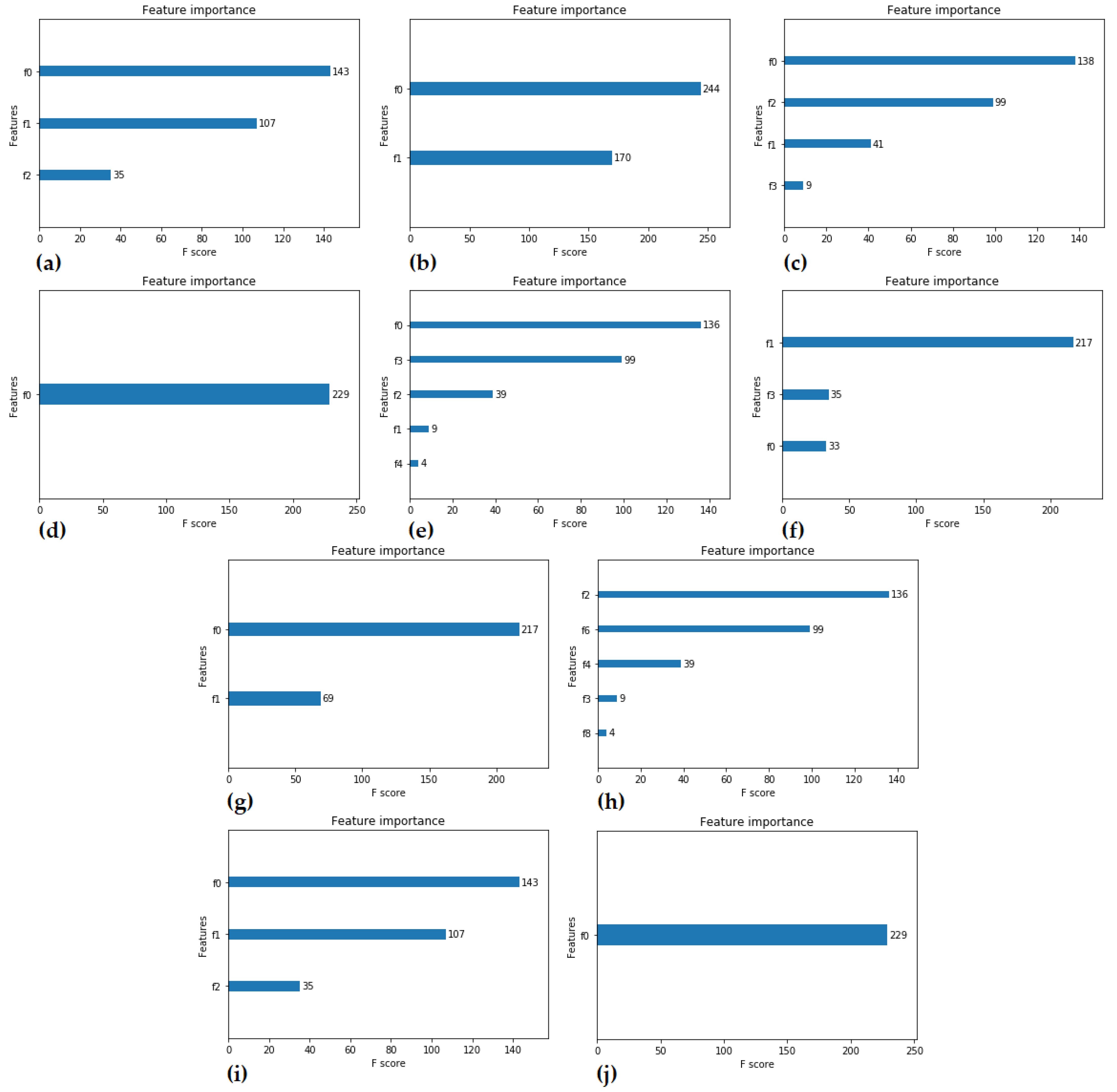
  • The feature-selection process uses feature significance ratings with the help of estimated feature importance from the used dataset. The training dataset is used to choose features, and then the model is trained using the selected features and evaluated on the test set. Both datasets were subjected to the XGBoost (XGB) feature importance to acquire a clear picture of the attribute relevance before selection;
  • Feature selection is a procedure in which you automatically pick those characteristics in your dataset that contribute the most to the output variables. The presence of irrelevant characteristics in your data might reduce the performance of many models. Feature selection before modeling not only improves accuracy but also reduces training time and the likelihood of overfitting. In this study, we implemented three popular attribute-selection techniques which are; SFM, RFE, and SKB;
  • The concept of a multilevel ensemble is introduced in this experimental work where the predictions of the bagging and boosting ensemble classifiers further undergo the voting ensemble with soft and hard voting. This methodology obtained state-of-the-art results on both proposed and open source datasets. For performance evaluation, multiple metrics such as recall, hamming loss, precision, etc., have been used.

1.2. Literature Review

In the healthcare industry, data-mining techniques such as classification, segmentation, correlation, clustering, and regression may be used to detect diseases [13]. Every year, a significant number of people are hospitalized with thyroid disorders. As a result, obtaining an early and accurate diagnosis is becoming increasingly challenging for healthcare facilities. The mentioned literature review will highlight several machine-learning techniques used to classify thyroid illness in various research. Nowadays, early detection and indications play a very crucial part in the effective diagnosis of various diseases. This requires the use of ML algorithms for accurate prediction. Mushtaq et al. [14] used the KNN algorithm for breast cancer classification. It provides a method for determining the distance between two sets of data. The performance of KNN is dependent on the K value, which is the number of adjacent entities. To discover an effective KNN, this research investigates KNN performance employing multiple distance functions and K values. There are multiple research domains in which researchers used different ML techniques for the better and more efficient detection and diagnosis of diseases.
The research in [15] employs two ML methods to identify thyroid conditions by using SVM and RF. The Thyroid Dataset from the University of California Irvine (UCI) was used for the investigation. Both methods were evaluated in terms of accuracy, recall, F-score, and precision. The SVM and RF models scored 91%, and 89% accuracies, respectively. Studies showed that SVM outperforms RF in the identification of thyroid issues. ML classifiers were used to predict thyroid issues in [16]. Data preparation techniques were adopted to make the data more basic so that algorithms could detect the risk of patients acquiring this disease. Machine learning is widely used for disease prediction. SVM, DT, LR, artificial neural network (ANN), and KNN are some of the approaches that scientists employ to predict if a patient may acquire thyroid illness. A website has been built to collect user input to provide educated estimations regarding type of illness. Sonuc et al. in [17] divided thyroid illness into three different groups based on data from Iraqi citizens, where some of them had an overactive thyroid and others had hypothyroidism. The SVM, DT, RF, NB, LR, KNN, and linear discriminant analysis (LDA), in addition to multilayer perceptron (MLP), was implemented to classify thyroid issues. The most accurate classifiers in descending order were RF, DT, NB, LR, KNN, and LDA, followed by MLP with 89 and 88% accuracy, respectively. The supervised learning approach was selected for inclusion in the study [18]. Anaconda and python platforms were used to create these algorithms for identifying the type of thyroid illness. The authors employed a variety of methods, including SVM, KNN, DT, naïve Bayes (NB), RF, and LR, among others. The results were plotted to evaluate how well LR matches up to RF in terms of accuracy. A low-cost thyroid diagnostic report is now available to patients using this technique. To identify thyroid texture, researchers in this study [19] offer three machine-learning-based methods known as the SVM, RF, and ANN. The researchers generated 30 spectral energy-based attributes for these classifiers during training via autoregressive modeling on a signal variant of 2D thyroid US pictures. Instead of using text-based descriptors, they employed image-based characteristics to illustrate thyroid tissues. When all three methods were used collectively, accuracy hovered around 90%.
Zhu et al. [20] proposed the use of ANN to develop a model for distinguishing benign from malignant nodules and for enhancing the accuracy of US-based objective diagnosis. Key sonographic markers and statistically significant changes made up the input layer of the ANN, which was utilized to predict nodule malignancy. The size, structure, echogenicity, internal composition, nodules, and peripheral halo of ultrasonography malignant nodules had a substantial association. When used on the training cohort, the ANN accurately predicted 82.3% of thyroid cancer cases with a value of 0.818 for area under the curve (AUC) and 84.5% accuracy rate. This method’s findings had an accuracy, sensitivity, and specificity of 83.1%, 83.8%, and 81.82 %, respectively, in the validation cohort. The AUC score for this investigation was 0.828. Clinical datasets were used in [21] and compared SVM, NB, and DT classifiers. The SVM algorithm is most extensively used in ML. Researchers mixed two feature selection techniques to compare the model’s performance. The filter technique was used first to pick the features, and the classifier’s effectiveness was assessed using the wrapper approach. The Fisher Discriminant Ratio (FDR) value was being used in binary classification to rank features based on significance. Three performance indicators were used to evaluate the addition of advanced features to the categorization model. Sequential forward and sequential backward selection are two well-known systematic attribute selection techniques, utilized in this case analysis [22]. In nonlinear optimization problems, the evolutionary method is a popular strategy for picking features. The SVM was used to detect hypothyroidism. Thyroid disease was examined using two distinct types of data in this study. The first dataset was used from the UCI repository, while the second dataset featured real data from the Imam Khomeini Hospital at the K. N. Toosi University of Technology’s Intelligent System Lab. To speed up CH diagnosis and therapy selection, a data-mining approach was applied by researchers. As a part of this cross-sectional study [23], authors deployed the SVM, MLP, Chi-Squared Automatic Interaction Detector (CHAID), and Iterative Dichotomiser-3 by integrating classification algorithm. By using the aforementioned classification methods, and bootstrap aggregating (Bagging), and boosting procedures, the negative impacts of dataset imbalance on classification outcomes were minimized. When using SVM-Bagging, precision and specificity were both 100%, the recall was 73.33%, and the F-measure was 84.62%. The investigative findings by authors in [24] revealed the DT attribute partitioning criteria for thyroid disease detection. Thyroid nodules may be effectively and efficiently classified using the method outlined below. In this study, methodologies such as DT, SVM, and NB were used to make a comparative diagnosis of thyroid illness. The accuracy goal for this classification is 99.89%. Previous attempts at employing the DT had disappointing results. Data from the UCI was used by Geetha et al. [25] in their analysis. The Hybrid Differential Evolution (HDE) kernel-based Naïve algorithm used high dimensionality to limit the existing 21 features to 10 attributes before running the algorithm. The accuracy of the kernel-based NB classification method has risen to 92% as a result of this development. As a hybrid model, it is critical to have a strong knowledge base that can be leveraged to tackle difficult learning tasks such as clinical diagnosis and prognostication. This research looked at a variety of ML methods and thyroid disease-prevention diagnostics in [26]. Depending on a patient’s medical history, algorithms such as SVM, KNN, and DT were employed to assess the risk of thyroid illness. A three-stage approach for treating thyroid illness was devised by another team of researchers led by Chen et al. in [27]. The author Fedushko et al. proposed a big-data- and operational intelligence-based system, including distinct machine-learning and preprocessing techniques for effective classification in [28]. The (FS-PSO-SVM) CAD technique with particle swarm optimization performed better than the current methods and obtained a precision of 98.59% by utilizing 10-fold cross-validation. Dogantekin et al. classified thyroid illness with an accuracy of 91.86% using feature extraction, and feature reduction classification phases with generalized discriminant analysis (GDA), and wavelet support vector machines (WSVM) [29]. The researchers Keleş et al. developed an expert system for the detection of thyroid illness termed as an expert system for thyroid disease diagnosis (ESTDD). The neuro-fuzzy classification (NEFCLASS) method was used to apply fuzzy rules, and the results showed 95.33% accuracy [30]. According to Ozyilmaz et al., using a variety of neural network approaches including back-propagation-based MLP, the radial-based function, and adaptive conic-section function in neural networks, thyroid diagnostic accuracy was shown to be 88% [31].

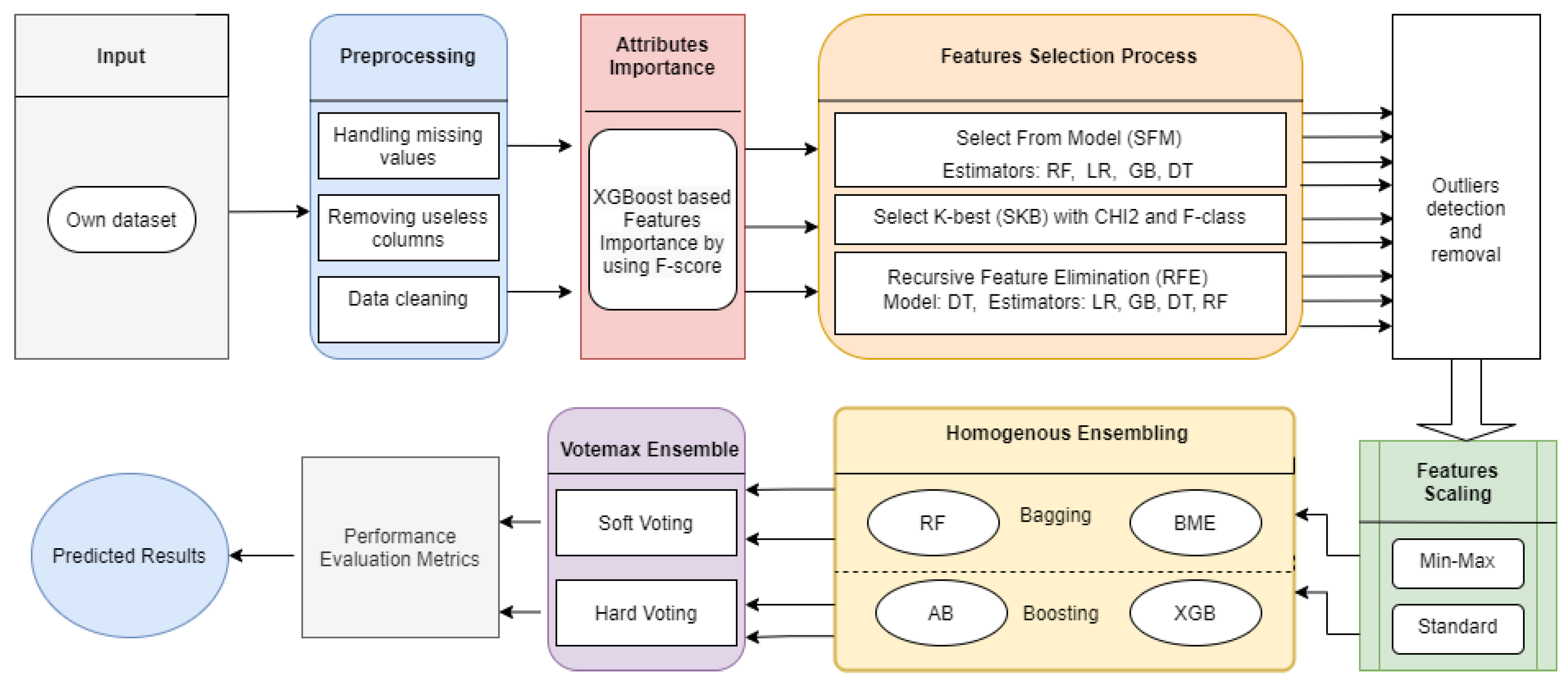
2. Materials and Methods

The research technique is shown in Figure 1. Before beginning the analysis, it is crucial to display and visualize the data. The purification, cleaning, and reduction of useless data, as well as missing values, can be accomplished by data preprocessing to improve the data representation and accuracy of the model. Next, we used XGBoost classifier to visually represent the importance of attributes based on the F-score [32]. Furthermore, the three used feature-selection techniques, SFM, SKB and RFE, are presented with their estimators in Figure 1.
The next step was the detection and removal of the outliers. It is very essential to detect and locate the outliers after attributes selection, hence the absence and presence of the outliers are proportional to the total number of selected features. The next step is to normalize the data from the selected features by using the scaling approach.
For this purpose, both standard and min–max scaling were implemented. Feature scaling is used to make the data more regular. Finally, the homogenous ensemble bagging (RF and Bagging Meta Estimator (BME)) and boosting (AdaBoost (AB) and XGB) are performed. After the classification, the predictions undergo the voting ensemble again, involving both soft and hard voting. The performance evaluation measures are further used for the clear assessment of implemented methodologies.

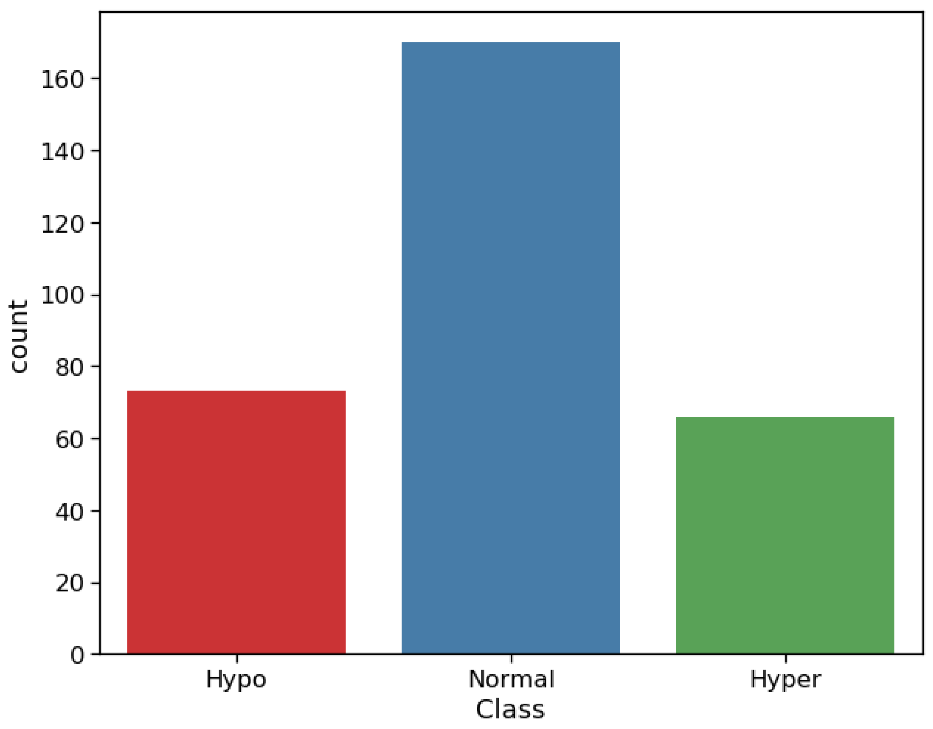
2.1. Dataset Description

This experimental research work focused on the dataset related to thyroid disease. The dataset was collected and gathered from a popular district headquarter hospital of the Punjab province, the city Dera Ghazi Khan, Pakistan. The dataset is carefully evaluated and verified by two expert endocrinologists from a well-known and famous hospital in Karachi, Pakistan [33]. The dataset contains 309 entities directly associated with the total number of subjects. Each person undergoes ten different screening tests that are further represented as features and one target variable represented as ‘Class’. This outcome variable is further categorized into three distinct classes expressed as ‘Hypo’ for Hypothyroidism, Normal, and Hyperthyroidism is denoted as ‘Hyper’. There is a total of 13 missing values represented as ‘?’ in a ‘T3’ feature. Table 1 shows the details of this dataset. The descriptions of the output variable and categories have been illustrated in Figure 2.

2.2. Data Preprocessing

The dataset used in this research study is in the form of a CSV file. Therefore, there is a chance of the missing values, and it had few useless columns such as the ‘Sr. No.’ and ‘Reference IDs’ of the patients. These attributes should be removed from the dataset as they do not have any specific impact on the outcome variable ‘Class’, and severely affect the performance of the models. This dataset also contains very few integer and real values, and most of the attribute details are in the form of strings and characters. Hence, it is difficult for the libraries to perform operations on these values directly. We convert these characters or strings into real numbers or integer values, for example, in ‘Pregnancy’ the value ‘Yes’ represented as 1 and ‘No’ is denoted as 0. All the remaining features have been changed in a similar aspect. The 13 missing values present in the ‘T3’ represented by ‘?’ were assigned with the mean values to obtain better performance. All the data cleaning process has been conducted in the preprocessing step.

2.3. XGBoost-Based Feature Importance by Using F-Score

Strategies that allocate a score to input features depending on how valuable they are at forecasting an outcome variable are known as feature importance. In a predictive modeling project, feature relevance scores play a significant role in providing information about the attributes and insight into the model. It lays the foundation of dimensionality reduction for high-dimensional data and attribute selection, which can increase the efficiency and efficacy of a forecasting model on the problem. Statistical correlation scores, coefficients generated as part of linear and regression models, RF and DT oriented attributes scores, permutation-based scores, and F-score-based attribute importance are some of the most commonly used methods [32]. Using the SFM class, the XGB-based feature importance is implemented [34], which takes a model and transforms it into a subset with chosen characteristics. It is possible to use a model that has already been trained using the complete training dataset with this method. When a threshold is reached, it can choose which attributes to use. SFM’s convert() function uses this threshold to ensure that features selected for training and testing are the same. The following example shows how to use XGB to first train and then test a model on a proposed dataset. The model is then wrapped in an SFM instance based on the feature importance determined from the training data. The training dataset is used to choose features, and the model is trained using the subset of features that have been selected. Finally, the model is evaluated on the test dataset and uses the same feature-selection methods as before. This technique is very helpful for a better diagnosis of thyroid disorder. Figure 3 illustrates the feature importance with the highest F-scores for the selected features by each attribute-selection technique.

2.4. Attribute Selection Approaches

The process of identifying the most reliable, nonredundant, most relevant characteristics for use in model development is known as feature selection. As the number and diversity of datasets expand, it is critical to reduce their size methodically. The primary objective of feature selection is to boost the effectiveness of a predictive model while lowering the modeling computational cost. The details of each feature-selection method have been discussed in Table 2.

2.4.1. Selection from Model (SFM)

The SFM is a meta-transformer that may be used in conjunction with any estimator that gives significance to each feature via a particular property (such as coef function, feature importance) or by an importance extractor. If the matching relevance of the attribute values is less than the specified threshold parameter, the characteristics are considered irrelevant and deleted. There are established mechanisms for calculating a threshold using a text input in addition to providing the threshold numerically. For example, "median", ’’mean’’ and fractional multiples of these, such as “0.1*mean” are available heuristics. In conjunction with the qualifying criteria, the max features option may be used to restrict the number of selected features. The implementation of SFM has been performed by using the sklearn package [35]. The estimators used in this approach are LR [36], RF [37], DT [38], GB [39].

2.4.2. Recursive Feature Elimination (RFE)

RFE is a feature-selection algorithm with a wrapper framework. This indicates that a distinct classification algorithm is provided and utilized in the method’s core, which is wrapped by RFE, and further used to assist in the feature selection process. This method contrasts with the filter-oriented attribute selection where each feature is selected based on the highest and lowest score. RFE is a wrapper-based method that internally employs filter-based characteristics selection. RFE finds a set of attributes by starting with all the features in the training sample and successfully eliminating features until the target number is reached. The whole attribute-selection procedure is achieved by fitting the provided ML algorithm employed in the model’s core, ranking features by significance, removing the least essential features, and refitting the model. This process is continued until only a certain number of characteristics remain. Features are rated using either the supplied ML model (e.g., some algorithms such as DT provide importance ratings) or a statistical technique. RFE is implemented in the sklearn ML package [35]. To obtain effective utilization of the RFE transformation, we first set up the class with the algorithm of choice provided by the “estimator” parameter and the number of attributes to pick via the “ n features to select” function. In this experimental study, the used core model is DT and the estimators are the same as discussed in Section 2.4.1, which are, LR, RF, DT, and GB.

2.4.3. Univariate Feature Selection Based Select K-Best (SKB)

In this approach, the statistical measures can be used to identify the characteristics with the strongest link to the output variable. The Select K-Best class in the sklearn package is used with a series of various statistical tests to pick a particular number of features. This research work selects the following best characteristics, as detailed in Table 2. The first method was based on the chi-squared (chi2) test that used the statistical or t analysis for non-negative features. The other parameter implemented in SKB is the f-class-if function denoted as (FCI), which calculates the ANOVA, and F-value for the sample that has been supplied.

2.5. Automatic Outlier Detection and Removal using Isolation Forest (ISO)

It is critical to purify the data samples before modeling to guarantee that the observations accurately reflect the situation. A dataset may comprise extreme values that are beyond the anticipated range and dissimilar to the rest of the data. These extreme independent values are known as the outliers. These are unique observations that stand out from the others. Understanding and even eliminating these outlier values can help enhance ML modeling and model ability in general. Because of the unique characteristics of each dataset, there is no exact technique to describe and detect outliers in general. The common practice includes the evaluation of the raw data and determining if a given result is an anomaly or not. Statistical techniques can be used to detect occurrences that appear to be unusual or implausible based on the available data. After that, the fit model will determine which samples in the training sample are outliers and which are inliers. The model will next be fitted to the remaining instances and assessed on the complete test dataset once the outliers have been eliminated from the training dataset. The ISO method is employed in this research, which is a tree-based outlier-detection method. It is based on modeling regular data in such a way that oddities that are both limited in number and distinct in feature space are isolated [40]. Table 3 represents the outlier detection in the dataset for each feature-selection technique with the mean absolute error (MAE).

2.6. Homogenous Ensemble

Ensemble techniques in ML and data mining employ several learning algorithms to achieve higher prediction performance than each of the individual learning algorithms alone. A homogenous ensemble is a series of classification models of the same type, where each is constructed on a distinct sample of data [41]. The two crucial types of the homogenous ensemble are bagging and boosting, which have been implemented in this research as initial ensembles.

2.6.1. Bagging

To improve accuracy, bagging is a method that significantly decreases the variation. As a result, overfitting is no longer an issue, which was a major problem with many prediction models. Homogeneous weak classifiers learn data in parallel, independently of one another, and then integrate them by averaging the results. Because the weak base classifiers are merged to produce a single but powerful classification model, the approach is more reliable than using single models. The biggest problem with these models is that they are computationally expensive. When we train a model, we obtain a function that takes an input, gives an output, and is defined concerning the training dataset, regardless of whether we are interacting with regression or a classification problem. The fitted model is also subject to variability due to the theoretical variation of the training dataset.
The concept of bagging is straightforward, where we want to build a model with a reduced variance by “averaging” the predictions from multiple different models. However, in practice, we are unable to build entirely independent models due to a large amount of required data. To fit almost independent models, we rely on the good “approximate characteristics” of bootstrap samples. This starts with creating several bootstrap samples, each one acting as a separate and nearly independent dataset taken from the real distribution. For each of these data, we may then train a weak learner, and eventually combine them such that their outputs are averaged, resulting in an ensemble classifier with reduced variation. Approximate independence and identical distribution are characteristics of bootstrap samples, and this is also true for learned base models. The bagging classifiers used in this research are as follows.
  • Random Forest (RF) [42];
  • Base Meta Estimator (BME) [43].

2.6.2. Boosting

This ensemble technique is the most commonly used and powerful. It was developed for classification issues and was later extended to include regression problems as well. The combined multiple weak models are no longer fitted separately from each other in sequential approaches. The aim is to fit models repeatedly so that the training of a model at each stage is dependent on the models fitted in prior phases. Boosting is the most well-known of these techniques, and it results in an ensemble model that is less biased than the weak learners that comprise it. AB, XGB, Gradient Boosting Machine (GBM), and Light GBM are the available boosting algorithms. In the case of boosting, if two models are predicted incorrectly then their outcomes are analyzed and combined for extraction of a better prediction. As a result, boosting demonstrates the ensemble fundamental concepts of transforming a weak classifier into a better one. The boosting models used in this research are:
  • AdaBoost (AB) [44];
  • XGBoost (XGB) [45].

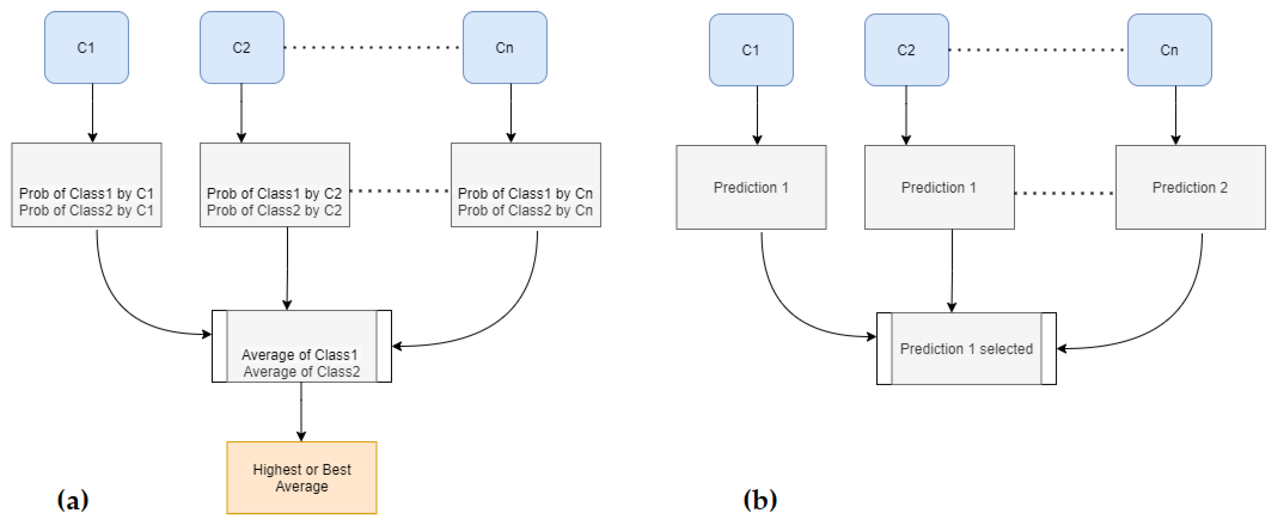
2.7. Voting Ensemble of Homogenous Ensemble

A voting ensemble (sometimes known as a "majority voting ensemble") is an ML ensemble model that incorporates predictions from many other models. It is a strategy that may be used to increase model performance, ideally outperforming any single model in the ensemble. The predictions from various models are combined in a voting ensemble. It may be used to classify or predict data. In the task of regression, this entails determining the average of the models’ predictions. In the event of categorization, the votes for each label are added together, and the label with the highest number of votes is predicted.
A voting ensemble can be thought of as a metamodel, or a model of models. It may be used as a metamodel with any collection of already trained ML models, and the existing models are not aware that they are being utilized in the ensemble. When we have two or even more models that execute a predictive modeling assignment well, a voting ensemble is ideal. The ensemble models must generally agree on their forecasts [46]. There are two ways to predict majority votes for classification, one method is hard voting and the other is soft voting [47]. Details of both voting techniques are as follows.

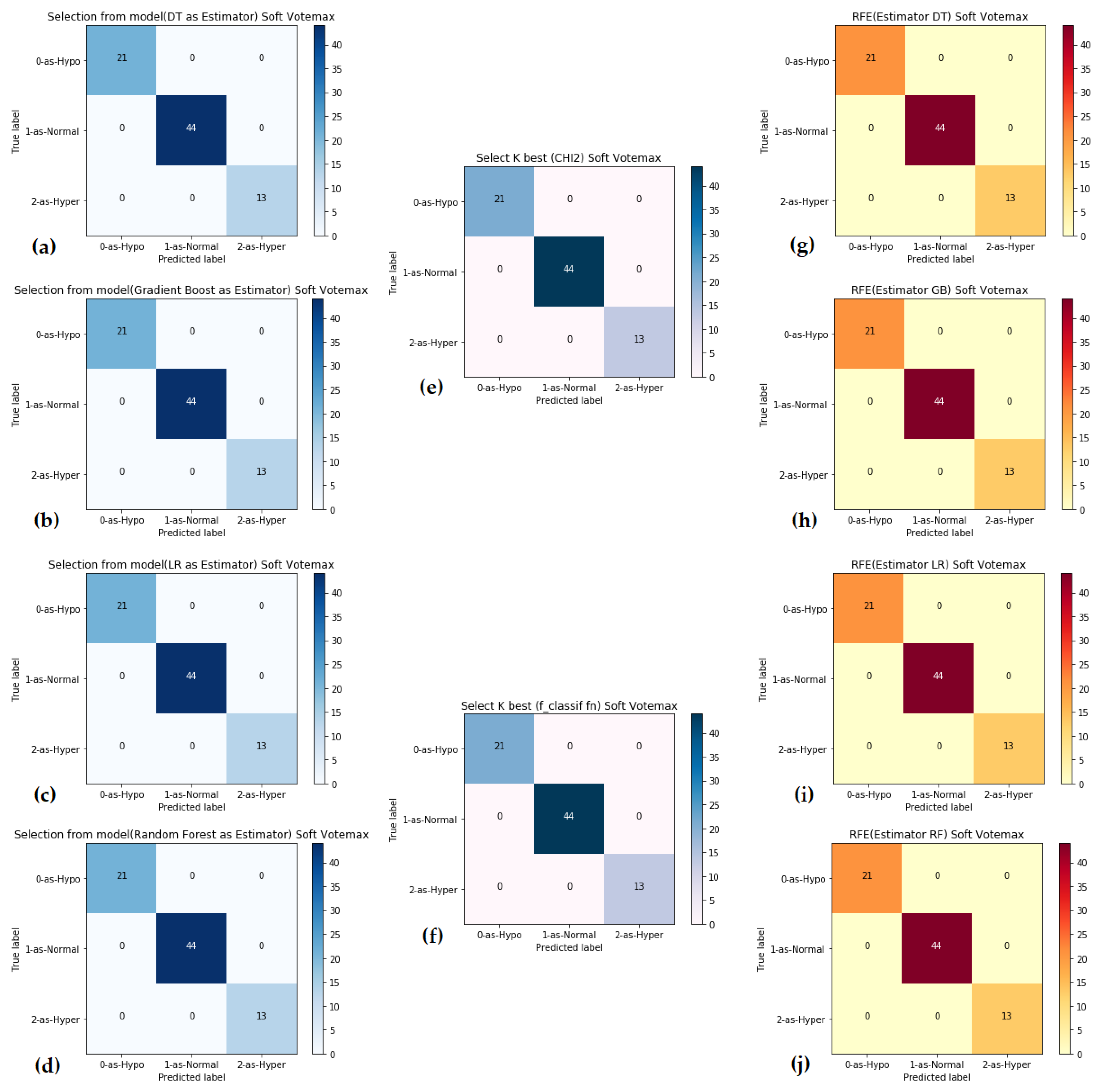
2.7.1. Soft Voting Ensemble

Figure 4a illustrates the soft voting process. Soft voting entails adding up the anticipated probabilities or scores for each target class estimating the class label with the greatest likelihood. It also predicts the class with the highest summed probability based on the models. Let us consider that the classifiers from C 1 , C 2 , C n and distribution of the probabilities for each classifier are P r o b m a x n and P r o b m i n n . Consider if the total number of classes is ‘two’ then the representation of these classes are C l a s s 1 = 0 and C l a s s 2 = 1 . The weight assignment for each classifier is denoted as W 1 , W 2 , W n . The calculation of the probabilities for the target class are as follows:
P r o b ( C l a s s 1 ) = W 1 P r o b m i n 1 + W 2 P r o b m i n 2 + + W n P r o b m i n n
P r o b ( C l a s s 2 ) = W 1 P r o b m a x 1 + W 2 P r o b m a x 2 + + W n P r o b m a x n
The averages of the target variable classes are calculated as:
A v g ( C l a s s 1 ) = ( P r o b m i n 1 + P r o b m i n 2 + + P r o b m i n n ) n
A v g ( C l a s s 2 ) = ( P r o b m a x 1 + P r o b m a x 2 + + P r o b m a x n ) n

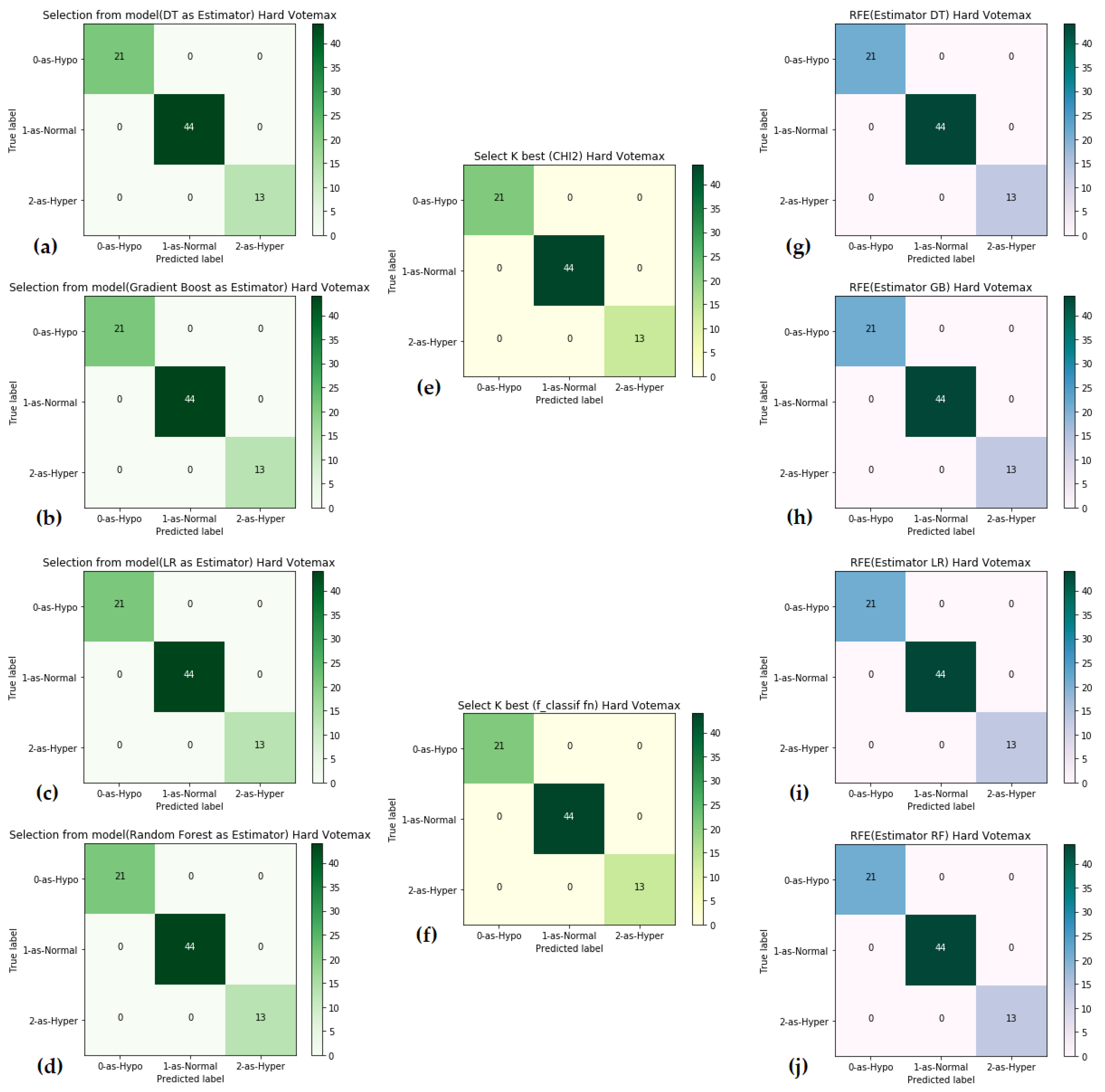
2.7.2. Hard Voting Ensemble

Hard voting entails adding up all the guesses for each class label and forecasting the class value with the most votes. In hard voting, we anticipate the class with the most votes from models. The mode of all predictions provided by multiple classifiers is used to classify input data using the hard voting classifier. When the weights associated with the distinct various algorithms are identical, majority voting is treated differently. In this case, consider again the total number of classifiers are n , represented as C 1 ,   C 2 ,   , C n whereas their predictions are denoted as P 0 and P 1 . The equation below and Figure 4b express the phenomena of hard voting classification.
| C 1 ,   C 2 ,   , C n |
| P 0 , P 0 , , P 1 |

2.8. Performance Assessment Metrics

Classification algorithms may be assessed in a variety of ways. Metrics analysis should be appropriately interpreted while assessing various learning methods. Some of the metrics generated from the confusion matrix are used to assess a diagnostic test for the classification of breast cancer [48,49] and human physiological conditions [50,51] using various ML classifiers. The confusion matrix includes a few key terms, such as A = True positive (TP), B = True negative (TN), C = False positive (FP), and D = False negative (FN). TP indicates that the system correctly predicts the outcome, and the outcome is also correct. The term FP refers to when the system predicts a right value, but the outcome is incorrect. TN indicates that the system predicts a false value, and the output is also a false value. The term FN refers to the system’s prediction that the outcome would be a false value when the outcome is a true value.

2.8.1. Confusion Matrix-Based Metrics

The most significant and often used metric for assessing classifier performance is accuracy which is calculated by dividing the number of accurate prediction samples by the total number of observations in the dataset.
A c c u r a c y = A + B A + B + C + D × 100 %
The ratio of genuine projected positive samples to the true positive samples is described as true positive rate (TPR) or recall.
S e n s i t i v i t y / R e c a l l / T P R = A A + D × 100 %
The F-measure is sometimes referred to as the F1-score. It explained the harmonic mean of accuracy and memory. A model is regarded as excellent if its score is one or it has a low false test rate, but a value of 0 indicates poor performance. The F1-score equation:
F 1   s c o r e = 2 A 2 A + C + D × 100 %
The Matthews correlation coefficient (MCC) was developed by Brain W. Matthews in 1975. This coefficient represents the connection between the observed and anticipated classifications. MCC is determined using the confusion matrix, and a + 1 number reflects flawless prediction, while a 1 value indicates a disagreement between forecasting and true values. MCC is defined below.
M C C = A × B C × D ( A + C ) ( A + D ) ( B + C ) ( B + D ) × 100 %
Precision or positive predictive value (PPV) is the percentage of relevant occurrences among the retrieved events.
P r e c i s i o n / P P V = A A + C × 100 %

2.8.2. Statistical Test

Cohen kappa is a statistical measure used to measure the degree of agreement between two evaluators. It may also be used to gauge how well a categorization model is doing in the real world.
c o h e n   k a p p a = p 0 p e 1 p e × 100 %
where p 0 represents the overall model accuracy, and p e represents the degree of agreement between the predicted values of the classes and the actual class values.

2.8.3. Loss and Error Finding

Mean absolute error (MAE) is a measure of how far off the original and forecasted values are from each other, and are averaged across the whole data set.
M A E = 1 N ( i = 1 N | Y i Y | ) × 100 %
Mean square error (MSE) reflects the difference between the actual and projected values, calculated by squaring the average difference across the whole dataset.
M S E = 1 N ( i = 1 N ( Y i Y ) 2 ) × 100 %
where Y i is the original value, Y represents the predicted value.
In statistics, the Hamming loss (HL) is the percentage of erroneously predicted labels.
H a m m i n g   L o s s = 1 | N | . | L | ( j = 1 | L | i = 1 | N | ( Y i , j Z i , j ) ) × 100 %
where Y i , j is equal to the target, and Z i , j denotes the forecasted value.

3. Results and Discussion

The proposed methodology of an ensemble of homogenous ensemble hybrids with three feature-selection approaches and multiple estimators is presented in this section. The experiment has been performed on the Jupyter notebook with a python platform involving multiple ML libraries and packages. The splitting method with a ratio of 75% training and 25% testing has been implemented, with hyperparameters tuned for the classifiers.
Table 4 demonstrates the accuracy of the RF and BME including their training and prediction time for each attribute-selection technique with the used estimator and function. It is clearly shown that all the classifiers obtained 100% accuracy with all the estimators in the implemented feature selection approaches. Only LR estimator from SFM attribute selection obtained 98.71% by using RF base learner. The lowest training and prediction time with 100% accuracy was attained by the RFE feature selection with DT estimator, only 01 selected feature, and the BME forecasting bagging model. The performance of the boosting predictors AB and XGB has been shown in Table 5. All the estimators with their feature-selection methods attained 100% accuracy. The exception is the FCI function in the SKB method with XGB classifier, which obtained 97.43% accuracy.
Table 6 reveals the second stage of the ensemble known as a voting ensemble with both soft and hard voting strategies. Although the computational cost of this ensemble stage is slightly higher than the first stage in terms of the accuracy and other implemented performance assessment measures, the proposed method attained a state-of-the-art result with zero error and loss and 100% precision, recall, MCC, kappa, etc. The proper implementation of the voting ensemble of homogenous ensemble refers to a minor delay in the computational operation due to the process of identifying the calculated or assigned weights and averages for the bagging and boosting classifiers in soft and hard voting.
Figure 5 represents the confusion matrices for the soft voting ensemble of the bagging (RF, BME) and boosting (AB, XGB) predictors. Soft voting involves equal weights for each classifier. Figure 5a–d represents the confusion matrices with SFM feature selection, whereas Figure 5e,f exhibit the SKB, and RFE is included in Figure 5g–j, illustrating the performance of each implemented estimator or function.
Similarly, Figure 6 illustrates the hard voting ensemble. Figure 6a–d represents the SFM, Figure 6e and Figure 6f denote SKB, and Figure 6g–j illustrates the confusion matrices for the RFE attribute-selection approach with the estimators.
As shown in Table 7, the method used in this research work has been investigated alongside other existing studies on the same dataset. The results of the proposed study were obtained by utilizing a variety of homogenous (bagging, boosting) ensembles with multiple feature-selection techniques. In this study, the researchers aimed for greater accuracy, reduced training, and prediction times. The hybrid implementation of the multiple feature selection, outlier, and anomaly detection with initial ensemble classifiers is performed by bagging and boosting techniques. The final prediction was conducted by another second stage of the ensemble process of the voting (soft and hard). The proposed method used a combination of complex algorithms and distinct strategies. This study attained the best results with higher accuracy, recall, and F1-score of 100% by utilizing less training and prediction time compared with existing hybrid models. This comparison concludes that existing approaches are not only more expensive to implement, but they also require more time to train and validate results.

4. Conclusions

The early detection and diagnosis of disease are critical for human survival. Recognition and identification have become more precise and accurate due to the use of machine-learning algorithms. Thyroid disease is difficult to diagnose because its symptoms can be mistaken for those of other ailments. New features in the thyroid dataset have a positive impact on classifier performance, and the results show that it provides better accuracy than previous studies. This research work focused on the implementation of the voting ensemble of a homogenous ensemble in combination with three separate attribute-selection techniques. The necessary preprocessing and detection of the outliers from the selected features were conducted before the classification process. The bagging and boosting ensembles contribute two algorithms for the initial ensemble. The bagging ensembles focused on the random forest and bagging meta estimator (BME) algorithms whereas the boosting ensemble implementation includes AdaBoost and XGBoost. Among all implemented ensemble techniques, the BME shows better performance by achieving the best accuracy in less training and prediction time. The consistency in the execution is independent of the total number of features selected for the datasets. In the second part of the classification, a voting ensemble with both hard and soft voting was implemented. Results show that all the feature-selection techniques, in combination with multiple estimators and ensemble techniques, attained the highest accuracy of 100% with a very low computational cost. Our proposed approach also obtained 100% results in terms of other used performance evaluation metrics. In comparison with existing studies, our method achieved the best results on the thyroid illness dataset.

Author Contributions

Conceptualization, methodology, and drafting, T.A., S.O.G., Z.M.; formal analysis, investigation, and validation, T.A., S.A., Z.M.; data curation, writing—review and editing, S.A., Z.M., A.W.; resources, supervision, and project administration, S.O.G., M.J., Y.A., and S.I.B. All authors have read and agreed to the published version of the manuscript.

Funding

This research received no external funding.

Institutional Review Board Statement

The study was conducted according to the latest guidelines of the Declaration of Helsinki. It was reviewed and approved by the Institutional Review Board of the Department of Robotics and Artificial Intelligence, School of Mechanical and Manufacturing Engineering, National University of Sciences and Technology, Pakistan.

Informed Consent Statement

Informed consent for participation was obtained from all subjects involved in the study. Written informed consent has been obtained from the patient(s) prior to publishing of this paper.

Data Availability Statement

The datasets analyzed in this article are not publicly available. Requests to access the datasets should be directed to [email protected].

Acknowledgments

The administrative and technical support from the District Head Quarter Hospital, Dera Ghazi Khan, Pakistan is acknowledged for providing the dataset and documentation for this study.

Conflicts of Interest

The authors declare no conflict of interest. It is declared that the research was conducted in the absence of any commercial or financial relationships that could be construed as a potential conflict of interest.

References

  1. American Thyroid Association. Thyroid Function Tests. Available online: https://www.thyroid.org/thyroid-function-tests/ (accessed on 15 August 2021).
  2. Shroff, S.; Pise, S.; Chalekar, P.; Panicker, S.S. Thyroid Disease Diagnosis: A Survey. In Proceedings of the 2015 IEEE 9th International Conference on Intelligent Systems and Control (ISCO), Coimbatore, India, 9–10 January 2015; pp. 1–6. [Google Scholar]
  3. Thyroid Cancer. Available online: https://seer.cancer.gov/statfacts/html/thyro.html (accessed on 1 September 2021).
  4. Ioniţă, I.; Ioniţă, L. Prediction of Thyroid Disease Using Data Mining Techniques. BRAIN Broad Res. Artif. Intell. Neurosci. 2016, 7, 115–124. [Google Scholar]
  5. Medline Plus. Hyperthyroidism, Graves, Disease, Overactive Thyroid, MedlinePlus. Available online: https://medlineplus.gov/hyperthyroidism.html (accessed on 15 August 2021).
  6. Sampath, P.; Packiriswamy, G.; Pradeep Kumar, N.; Shanmuganathan, V.; Song, O.Y.; Tariq, U.; Nawaz, R. IoT Based health—Related topic recognition from emerging online health community (med help) using machine learning technique. Electronics. 2020, 9, 1469. [Google Scholar] [CrossRef]
  7. Reid, J.R.; Wheeler, S.F. Hyperthyroidism: Diagnosis and Treatment. Am. Fam. Physician 2005, 72, 623–630. [Google Scholar]
  8. Pal, R.; Anand, T.; Dubey, S.K. Evaluation and Performance Analysis of Classification Techniques for Thyroid Detection. Int. J. Bus. Inf. Syst. 2018, 28, 163–177. [Google Scholar] [CrossRef]
  9. Prasad, V.; Rao, T.S.; Babu, M.S.P. Thyroid Disease Diagnosis via Hybrid Architecture Composing Rough Data Sets Theory and Machine Learning Algorithms. Soft Comput. 2016, 20, 1179–1189. [Google Scholar] [CrossRef]
  10. Healthline. Thyroid Functions Tests. Available online: https://www.healthline.com/health/thyroid-function-tests (accessed on 15 August 2021).
  11. Singh, N.; Jindal, A.A. Segmentation Method and Comparison of Classification Methods for Thyroid Ultrasound Images. Int. J. Comput. Appl. 2012, 50, 43–49. [Google Scholar] [CrossRef]
  12. Erol, R.; Oğulata, S.N.; Şahin, C.; Alparslan, Z.N. A Radial Basis Function Neural Network (RBFNN) Approach for Structural Classification of Thyroid Diseases. J. Med. Syst. 2008, 32, 215–220. [Google Scholar] [CrossRef] [PubMed]
  13. Begum, A.; Parkavi, A. Prediction of Thyroid Disease Using Data Mining Techniques. In Proceedings of the 2019 5th International Conference on Advanced Computing & Communication Systems (ICACCS), Coimbatore, India, 15–16 March 2019; pp. 342–345. [Google Scholar]
  14. Mushtaq, Z.; Yaqub, A.; Sani, S.; Khalid, A. Effective K-Nearest Neighbor Classifications for Wisconsin Breast Cancer Data Sets. J. Chin. Inst. Eng. 2020, 43, 80–92. [Google Scholar] [CrossRef]
  15. Shivastuti, H.K.; Manhas, J.; Sharma, V. Performance Evaluation of SVM and Random Forest for the Diagnosis of Thyroid Disorder. Int. J. Res. Appl. Sci. Eng. Technol. 2021, 9, 945–947. [Google Scholar]
  16. Zhang, B.; Tian, J.; Pei, S.; Chen, Y.; He, X.; Dong, Y.; Zhang, L.; Mo, X.; Huang, W.; Cong, S. Machine Learning—Assisted System for Thyroid Nodule Diagnosis. Thyroid 2019, 29, 858–867. [Google Scholar] [CrossRef]
  17. Sonuç, E. Thyroid Disease Classification Using Machine Learning Algorithms. J. Phys. Conf. Ser. 2021, 1963, 012140. [Google Scholar]
  18. Yadav, D.C.; Pal, S. Thyroid Prediction Using Ensemble Data Mining Techniques. Int. J. Inf. Technol. 2019, 1–11. [Google Scholar] [CrossRef]
  19. Poudel, P.; Illanes, A.; Ataide, E.J.; Esmaeili, N.; Balakrishnan, S.; Friebe, M. Thyroid Ultrasound Texture Classification Using Autoregressive Features in Conjunction with Machine Learning Approaches. IEEE Access 2019, 7, 79354–79365. [Google Scholar] [CrossRef]
  20. Zhu, L.-C.; Ye, Y.-L.; Luo, W.-H.; Su, M.; Wei, H.-P.; Zhang, X.-B.; Wei, J.; Zou, C.-L. A model to Discriminate Malignant from Benign Thyroid Nodules Using Artificial Neural Network. PLoS ONE 2013, 8, e82211. [Google Scholar] [CrossRef] [PubMed]
  21. Singh, A.K. A Comparative Study on Disease Classification Using Machine Learning Algorithms. In Proceedings of the 2nd International Conference on Advanced Computing and Software Engineering (ICACSE), Sultanpur, India, 8–9 February 2019. [Google Scholar]
  22. Kousarrizi, M.N.; Seiti, F.; Teshnehlab, M. An Experimental Comparative Study on Thyroid Disease Diagnosis Based on Feature Subset Selection and Classification. Int. J. Electr. Comput. Sci. IJECS-IJENS 2012, 12, 13–20. [Google Scholar]
  23. Mousavi, S.S.Z.; Zanjireh, M.M.; Oghbaie, M. Applying Computational Classification Methods to Diagnose Congenital Hypothyroidism: A Comparative Study. Inf. Med. Unlocked 2020, 18, 100281. [Google Scholar] [CrossRef]
  24. Nguyen, D.T.; Kang, J.K.; Pham, T.D.; Batchuluun, G.; Park, K.R. Ultrasound Image-Based Diagnosis of Malignant Thyroid Nodule Using Artificial Intelligence. Sensors 2020, 20, 1822. [Google Scholar] [CrossRef] [PubMed] [Green Version]
  25. Geetha, K.; Baboo, S.S. An Empirical Model for Thyroid Disease Classification Using Evolutionary Multivariate Bayseian Prediction Method. Glob. J. Comput. Sci. Technol. 2016, 16, 1–10. [Google Scholar]
  26. Chaubey, G.; Bisen, D.; Arjaria, S.; Yadav, V. Thyroid Disease Prediction Using Machine Learning Approaches. Natl. Acad. Sci. Lett. 2021, 44, 233–238. [Google Scholar] [CrossRef]
  27. Chen, H.-L.; Yang, B.; Wang, G.; Liu, J.; Chen, Y.-D.; Liu, D.-Y. A Three-Stage Expert System Based on Support Vector Machines for Thyroid Disease Diagnosis. J. Med. Syst. 2012, 36, 1953–1963. [Google Scholar] [CrossRef]
  28. Fedushko, S.; Ustyianovych, T.; Gregus, M. Real-Time High-Load Infrastructure Transaction Status Output Prediction Using Operational Intelligence and Big Data Technologies. Electronics 2020, 9, 668. [Google Scholar] [CrossRef] [Green Version]
  29. Dogantekin, E.; Dogantekin, A.; Avci, D. An Expert System Based on Generalized Discriminant Analysis and Wavelet Support Vector Machine for Diagnosis of Thyroid Diseases. Expert Syst. Appl. 2011, 38, 146–150. [Google Scholar] [CrossRef]
  30. Keleş, A.; Keleş, A. ESTDD: Expert System for Thyroid Diseases Diagnosis. Expert Syst. Appl. 2008, 34, 242–246. [Google Scholar] [CrossRef]
  31. Ozyilmaz, L.; Yildirim, T. Diagnosis of Thyroid Disease Using Artificial Neural Network Methods. In Proceedings of the 9th International Conference on Neural Information Processing, 2002. ICONIP’02, Singapore, 18–22 November 2002; pp. 2033–2036. [Google Scholar]
  32. Valko, M.; Hauskrecht, M. Feature Importance Analysis for Patient Management Decisions. Stud. Health Technol. Inform. 2010, 160, 861. [Google Scholar]
  33. Abbad Ur Rehman, H.; Lin, C.-Y.; Mushtaq, Z. Effective K-Nearest Neighbor Algorithms Performance Analysis of Thyroid Disease. J. Chin. Inst. Eng. 2021, 44, 77–87. [Google Scholar] [CrossRef]
  34. Brownlee, J. Feature Importance and Feature Selection with XGBoost in Python. Machine Learning Mastery. Available online: https://machinelearningmastery.com/feature-importance-and-feature-selection-with-xgboost-in-python/ (accessed on 15 October 2021).
  35. Hao, J.; Ho, T.K. Machine Learning Made Easy: A Review of Scikit-Learn Package in Python Programming Language. J. Educ. Behav. Stat. 2019, 44, 348–361. [Google Scholar] [CrossRef]
  36. Seddik, A.F.; Shawky, D.M. Logistic Regression Model for Breast Cancer Automatic Diagnosis. In Proceedings of the 2015 SAI Intelligent Systems Conference (IntelliSys), London, UK, 10–11 November 2015; pp. 150–154. [Google Scholar]
  37. Dikshit, A.; Pradhan, B.; Alamri, A.M. Short-Term Spatio-Temporal Drought Forecasting Using Random Forests Model at New South Wales, Australia. Appl. Sci. 2020, 10, 4254. [Google Scholar] [CrossRef]
  38. Chowdhary, C.L.; Mittal, M.; Pattanaik, P.; Marszalek, Z. An Efficient Segmentation and Classification System in Medical Images Using Intuitionist Possibilistic Fuzzy C-Mean Clustering and Fuzzy SVM Algorithm. Sensors 2020, 20, 3903. [Google Scholar] [CrossRef] [PubMed]
  39. Wang, X.; Gong, G.; Li, N. Automated Recognition of Epileptic EEG States Using a Combination of Symlet Wavelet Processing, Gradient Boosting Machine, and Grid Search Optimizer. Sensors 2019, 19, 219. [Google Scholar] [CrossRef] [Green Version]
  40. Brownlee, J. Data Preparation for Machine Learning: Data Cleaning, Feature Selection, and Data Transforms in Python. Machine Learning Mastery. 2020. Available online: https://machinelearningmastery.com/data-preparation-for-machine-learning/ (accessed on 15 October 2021).
  41. Lal, A.; Datta, B. Performance Evaluation of Homogeneous and Heterogeneous Ensemble Models for Groundwater Salinity Predictions: A regional-Scale Comparison Study. Water Air Soil Pollut. 2020, 231, 1–21. [Google Scholar] [CrossRef]
  42. Wen, L.; Hughes, M. Coastal Wetland Mapping Using Ensemble Learning Algorithms: A Comparative Study of Bagging, Boosting and Stacking Techniques. Remote Sens. 2020, 12, 1683. [Google Scholar] [CrossRef]
  43. Alam, M.Z.; Rahman, M.S.; Rahman, M.S. A Random Forest Based Predictor for Medical Data Classification Using Feature Ranking. Inform. Med. Unlocked 2019, 15, 100180. [Google Scholar] [CrossRef]
  44. Palacios-Navarro, G.; Hogan, N. Head-Mounted Display-Based Therapies for Adults Post-Stroke: A Systematic Review and Meta-Analysis. Sensors 2021, 21, 1111. [Google Scholar] [CrossRef] [PubMed]
  45. Shen, Z.; Wu, Q.; Wang, Z.; Chen, G.; Lin, B. Diabetic Retinopathy Prediction by Ensemble Learning Based on Biochemical and Physical Data. Sensors 2021, 21, 3663. [Google Scholar] [CrossRef] [PubMed]
  46. Liew, X.Y.; Hameed, N.; Clos, J. An Investigation of XGBoost-Based Algorithm for Breast Cancer Classification. Mach. Learn. Appl. 2021, 6, 100154. [Google Scholar] [CrossRef]
  47. Brownlee, J. How to Develop Voting Ensembles with Python. Machine Learning Mastery. Available online: https://machinelearningmastery.com/voting-ensembles-with-python/ (accessed on 15 October 2021).
  48. Mushtaq, Z.; Yaqub, A.; Hassan, A.; Su, S.F. Performance Analysis of Supervised Classifiers Using PCA Based Techniques on Breast Cancer. In Proceedings of the 2019 International Conference on Engineering and Emerging Technologies (ICEET), Lahore, Pakistan, 21–23 February 2019; pp. 1–6. [Google Scholar]
  49. Sahu, B.; Mohanty, S.; Rout, S. A Hybrid Approach for Breast Cancer Classification and Diagnosis. EAI Endorsed Trans. Scalable Inf. Syst. 2019, 6, e2. [Google Scholar] [CrossRef]
  50. Arif, S.; Khan, M.J.; Naseer, N.; Hong, K.-S.; Sajid, H.; Ayaz, Y. Vector Phase Analysis Approach for Sleep Stage Classification: A Functional Near-Infrared Spectroscopy-Based Passive Brain-Computer Interface. Front. Hum. Neurosci. 2021, 15, 658444. [Google Scholar] [CrossRef]
  51. Arif, S.; Arif, M.; Munawar, S.; Ayaz, Y.; Khan, M.J.; Naseer, N. EEG Spectral Comparison between Occipital and Prefrontal Cortices for Early Detection of Driver Drowsiness. In Proceedings of the 2021 International Conference on Artificial Intelligence and Mechatronics Systems (AIMS), Bandung, Indonesia, 28–30 April 2021; pp. 1–6. [Google Scholar]
  52. Rehman, H.A.U.; Lin, C.-Y.; Mushtaq, Z.; Su, S.-F. Performance Analysis of Machine Learning Algorithms for Thyroid Disease. Arab. J. Sci. Eng. 2021, 46, 9437–9449. [Google Scholar] [CrossRef]
Figure 1. General block diagram of the proposed methodology for the diagnosis of thyroid illness.
Electronics 10 03026 g001
Figure 2. Details of the ‘Class’ variable categories of the dataset.
Electronics 10 03026 g002
Figure 3. Feature importance by using XGBoost based on F-scores for the selected attributes via used feature-selection techniques, (ad) The selected features for SFM using RF, LR, GB, DT, (e,f) for SKB using Chi2, FCI, (gj) attributes selection for RFE using RF, LR, GB, DT, respectively.
Electronics 10 03026 g003
Figure 4. Ensemble phenomena: (a) soft voting, (b) hard voting.
Electronics 10 03026 g004
Figure 5. Confusion matrices for the soft voting ensemble of the bagging and boosting classifiers by implementing various attribute-selection methodologies with multiple estimators. (ad) DT, GB, LR, RF estimators with SFM feature selection, (e) Chi2, (f) FCI with SKB feature selection, and (gj) DT, GB, LR, RF estimators with RFE attribute selection, respectively.
Electronics 10 03026 g005
Figure 6. Confusion matrices for the hard voting ensemble of the bagging and boosting classifiers by implementing various attribute-selection methodologies with multiple estimators. (ad) DT, GB, LR, RF estimators with SFM feature selection, (e) Chi2, (f) FCI with SKB feature selection, and (gj) DT, GB, LR, RF estimators with RFE attribute selection, respectively.
Electronics 10 03026 g006
Table 1. Details about the dataset related to thyroid disorders from the registered hospital.
Thyroid Dataset
Attributes NamesRange of Features
Serial Numbers1 to 309
Hospital Reference IDsUnique Number
PregnancyYes, No
Body Mass Index (BMI)Overweight
Optimal
Underweight
Blood Pressure (BP)Low
Healthy
High
Pulse Rate (PR)50 to 110
T30.15 TO 3.7
(Having 13 Missing values denoted by ‘?’)
TSH0.05 to 100
T40.015 to 30
GenderFemale
Male
Age6 to 62
Class‘0’ as Hypo
‘1’ as Hyper
‘2’ as Normal
Table 2. Details of the attributes selected by the feature-selection approach with the execution time.
Features Selection TechniquesEstimators or Functions UsedTotal Features in the Dataset after CleaningSelected FeaturesTime Required for Features Selection (s)
Select From Model (SFM)LR09020.010
RF09030.135
DT09010.032
GB09040.154
Select K Best
(SKB)
Chi209050.014
FCI09030.006
Recursive Feature Elimination
(RFE)
LR09050.092
RF09020.235
DT09010.010
GB09031.172
Table 3. Detail of the detected outliers and MAE values in the selected features.
Feature-Selection TechniqueEstimator or Function UsedTotal Features in the Dataset after CleaningTotal Entries Present in the DatasetEntities in 75% Training of the DataNumber of Selected FeaturesOutliers Detected in the Selected FeaturesMAE
Values
Select From Model (SFM)LR0930923102230.0001
RF0930923103230.0001
DT093092310100.0001
GB0930923104230.0001
Select K Best
(SKB)
Chi20930923105230.0001
FCI0930923103220.026
Recursive Feature Elimination
(RFE)
LR0930923105230.0001
RF0930923102190.295
DT093092310100.0001
GB0930923103230.0001
Table 4. Description of the accuracy with training and prediction time for the bagging classifiers.
Homogenous Ensemble (Bagging)
Feature-Selection TechniquesEstimators or Functions UsedSelected FeaturesBagging ClassifiersAccuracy (%)Training
Time (s)
Prediction
Time (s)
Select From Model (SFM)LR02RF98.710.28690.0029
BME100.00.01490.0020
RF03RF100.00.08610.0079
BME100.00.01390.0009
DT01RF100.00.30400.0029
BME100.00.02690.0019
GB04RF100.00.08730.0079
BME100.00.28440.0009
Select K Best
(SKB)
Chi205RF100.00.06430.0039
BME100.00.01080.0019
FCI03RF100.00.07430.0049
BME100.00.03290.0050
Recursive Feature Elimination
(RFE)
LR05RF100.00.02890.0030
BME100.00.00890.0009
RF02RF100.00.02590.0029
BME100.00.01290.0019
DT01RF100.00.03200.0039
BME100.00.01290.0009
GB03RF100.00.03290.0049
BME100.00.01290.0020
Table 5. Description of the accuracy with training and prediction time for the boosting classifiers.
Homogenous Ensemble (Boosting)
Feature-Selection TechniquesEstimators or Functions UsedSelected FeaturesBoosting ClassifiersAccuracy (%)Training
Time (s)
Prediction
Time (s)
Select From Model (SFM)LR02AB100.00.10370.0049
XGB100.00.98980.0009
RF03AB100.00.10470.0050
XGB100.01.31600.0019
DT01AB100.00.04900.0059
XGB100.01.33540.0009
GB04AB100.00.11870.0049
XGB100.00.97520.0008
Select K Best
(SKB)
Chi205AB100.00.07570.0049
XGB100.01.06820.0216
FCI03AB100.00.06780.0069
XGB97.431.00340.0009
Recursive Feature
Elimination
(RFE)
LR05AB100.00.05940.0059
XGB100.01.04840.0009
RF02AB100.00.06280.0059
XGB100.01.06140.0009
DT01AB100.00.09270.0049
XGB100.01.15960.0009
GB03AB100.00.06380.0059
XGB100.01.04720.0019
Table 6. Performance assessment measures for the soft and hard voting of the homogenous ensemble classifiers.
Ensemble of the Homogenous Ensemble (Voting Classifier)
Feature-Selection TechniquesEstimators or Functions usedSelected FeaturesVoting
Classifiers
Accuracy (%)Training
Time (s)
Prediction
Time (s)
Recall (%)Precision (%)F1-score (%)MCC (%)Cohen
Kappa (%)
MSE (%)MAE (%)Hamming
Loss (%)
Select From Model (SFM)LR02Soft100.01.0620.007100.0100.0100.0100.0100.00.00.00.0
Hard100.01.1030.007100.0100.0100.0100.0100.00.00.00.0
RF03Soft100.00.1760.010100.0100.0100.0100.0100.00.00.00.0
Hard100.00.1520.009100.0100.0100.0100.0100.00.00.00.0
DT01Soft100.01.4150.010100.0100.0100.0100.0100.00.00.00.0
Hard100.01.2160.014100.0100.0100.0100.0100.00.00.00.0
GB04Soft100.00.1900.009100.0100.0100.0100.0100.00.00.00.0
Hard100.01.0600.009100.0100.0100.0100.0100.00.00.00.0
Select K Best
(SKB)
Chi205Soft100.00.2080.015100.0100.0100.0100.0100.00.00.00.0
Hard100.00.3750.008100.0100.0100.0100.0100.00.00.00.0
FCI03Soft100.00.1590.013100.0100.0100.0100.0100.00.00.00.0
Hard100.00.1750.022100.0100.0100.0100.0100.00.00.00.0
Recursive Feature Elimination
(RFE)
LR05Soft100.01.0950.031100.0100.0100.0100.0100.00.00.00.0
Hard100.01.1380.009100.0100.0100.0100.0100.00.00.00.0
RF02Soft100.01.1250.009100.0100.0100.0100.0100.00.00.00.0
Hard100.01.3630.011100.0100.0100.0100.0100.00.00.00.0
DT01Soft100.01.1020.011100.0100.0100.0100.0100.00.00.00.0
Hard100.01.2300.010100.0100.0100.0100.0100.00.00.00.0
GB03Soft100.01.0870.016100.0100.0100.0100.0100.00.00.00.0
Hard100.01.0730.011100.0100.0100.0100.0100.00.00.00.0
Table 7. The comparison of the performance evaluation metrics and computational cost of the proposed research methodology with existing studies.
Ref.MethodologyAccuracy (%)Recall (%)F1-Score (%)Training Time (s)Prediction Time (s)Dataset
[52]KNN + WLSVC (L1)97.896970.530.361DHQ, DG Khan,
Pakistan
DT + WLSVC (L2)76.967610.6810.372
SVM + WLSVC (L2)86.079850.5110.361
[33]KNN (Euclidean) + WCHI1001001001.0320.806DHQ, DG Khan,
Pakistan
KNN (Minkowski) + WCHI99.399991.180.827
KNN (Chebyshev) + WCHI98.797981.110.808
KNN (Manhattan) + WCHI99.399991.010.749
KNN (Correlation) + WCHI77.376760.8990.655
This studyHomogenous ensemble + Voting (hard) + SFM (RF)1001001000.1520.009DHQ, DG Khan,
Pakistan
Homogenous ensemble + Voting (soft) + SKB (FCI)1001001000.1590.013
Bagging (BME) + RFE (DT)1001001000.01290.0009
Homogenous ensemble + Voting (hard) + RFE (GB)1001001001.0730.011
Publisher’s Note: MDPI stays neutral with regard to jurisdictional claims in published maps and institutional affiliations.

