Review

A Survey on EEG Signal Processing Techniques and Machine Learning: Applications to the Neurofeedback of Autobiographical Memory Deficits in Schizophrenia

by
Miguel Ángel Luján
1,
María Verónica Jimeno
2,
Jorge Mateo Sotos
1,
Jorge Javier Ricarte
2 and
Alejandro L. Borja
1,*
1
Departamento de Ingeniería Eléctrica, Electrónica, Automática y Comunicaciones, Universidad de Castilla-La Mancha, 02071 Albecete, Spain
2
Departamento de Psicología, Universidad de Castilla-La Mancha, 02071 Albecete, Spain
*
Author to whom correspondence should be addressed.
Submission received: 27 October 2021 / Revised: 29 November 2021 / Accepted: 2 December 2021 / Published: 5 December 2021

Abstract

:
In this paper, a general overview regarding neural recording, classical signal processing techniques and machine learning classification algorithms applied to monitor brain activity is presented. Currently, several approaches classified as electrical, magnetic, neuroimaging recordings and brain stimulations are available to obtain neural activity of the human brain. Among them, non-invasive methods like electroencephalography (EEG) are commonly employed, as they can provide a high degree of temporal resolution (on the order of milliseconds) and acceptable space resolution. In addition, it is simple, quick, and does not create any physical harm or stress to patients. Concerning signal processing, once the neural signals are acquired, different procedures can be applied for feature extraction. In particular, brain signals are normally processed in time, frequency, and/or space domains. The features extracted are then used for signal classification depending on its characteristics such us the mean, variance or band power. The role of machine learning in this regard has become of key importance during the last years due to its high capacity to analyze complex amounts of data. The algorithms employed are generally classified in supervised, unsupervised and reinforcement techniques. A deep review of the most used machine learning algorithms and the advantages/drawbacks of most used methods is presented. Finally, a study of these procedures utilized in a very specific and novel research field of electroencephalography, i.e., autobiographical memory deficits in schizophrenia, is outlined.

1. Introduction

The brain is the most complex organ and is composed of billion neurons and trillions of connections called synapses. Its main functions include the interpretation of external information and governing many aspects, such as intelligence, creativity, emotion, and memory. As a consequence of all this activity, neurons produce ionic currents and electric signals resulting in small voltage fluctuations. These signals are generally time-varying, non-Gaussian, non-stationary, random, and are often non-linear in nature [1,2]. Therefore, the measuring and monitoring of electrical activity in the brain is of primary importance as it can provide profound information related to the physiological, functional, and pathological status of the brain. It can be very useful for the identification of brain rhythms, diagnosis of brain disorders, detection of brain impairments, and consequently the possibility to provide, in some cases, precise treatment to correct or improve certain brain-health conditions in patients [3,4,5].
In this regard, the general process followed in medical studies to extract, analyze, and classify the brain signals can be observed in Figure 1. This process is commonly divided into four steps, signal acquisition, preprocessing, feature extraction, and classification [6], which are described as follows.
First, brain signals should be acquired for a later analysis. As will be shown, different methods can be employed by means of the use of several electrodes situated on the surface of the scalp or inside the brain. Thereafter, the stored data have to be preprocessed as it surely is modified by noise and external interferences. The noise present in the signal is due to the electrical distribution network, surrounding electronic equipment, or may be due to body functions, e.g., body movements, eye-blinking, breathing, or sweating. To remove noise components present in the signal proper filtering techniques can be used [7,8,9]. Once the brain signal is clear of interference and artifacts, feature extraction is performed [10,11,12] due to the huge volume of EEG signal data collected, which makes its direct processing extremely complicated. Feature extraction aims to reduce the amount of data by creating new features from the initial measured dataset that are non-redundant, contain the relevant information of the input data, and permit better classification by means of reduced representation obtained instead of the complete initial set of raw data [12]. Feature extraction is required to decrease the data dimensionality, thus transforming a set of data from a high-dimensional space into a low-dimensional space. This low-dimensional representation preserves the more significant properties of the original data. In this regard, operating in high-dimensional spaces is normally undesirable as raw data are often sparse, present redundant information, and take up a lot of hard drive resources. Then, the characteristics of the measured simplified signal can be tested, either in the time and/or frequency domain for classification during the execution of machine learning methods. Machine learning procedures involve the use of training data collection, with or without known results to develop algorithms that can learn from historical data and improve the system through experience. As a result, a classification method to compare certain feature signal characteristics can be developed to make predictions or decisions [13,14,15,16,17,18], for instance, to provide diagnosis of mental diseases/impairments.
In this paper, the digital techniques and machine learning methods generally employed during brain signal processing are presented. In addition, autobiographical memory and a deep analysis of different studies devoted to signal processing in this research field are shown. More specifically, the paper is divided into the following sections: In Section 2 and Section 3, the methods employed for signal acquisition and signal processing are presented, respectively. First, the methods and arrangements used to obtain the brain signals and how to treat the data acquired are considered to demonstrate EEG principle and basic properties. Next, the most popular techniques employed in EEG signal processing are studied. Section 4 shows the machine learning techniques that can be applied in EEG applications for classification. Section 5 presents how all these processes, i.e., EEG signal processing and machine learning, have been applied to determine the main characteristics of autobiographical memory up to the present. It also describes the experimental results and their interpretation, as well as experimental outlines obtained in previous research. Finally, the conclusions of the work are summarized in Section 6.

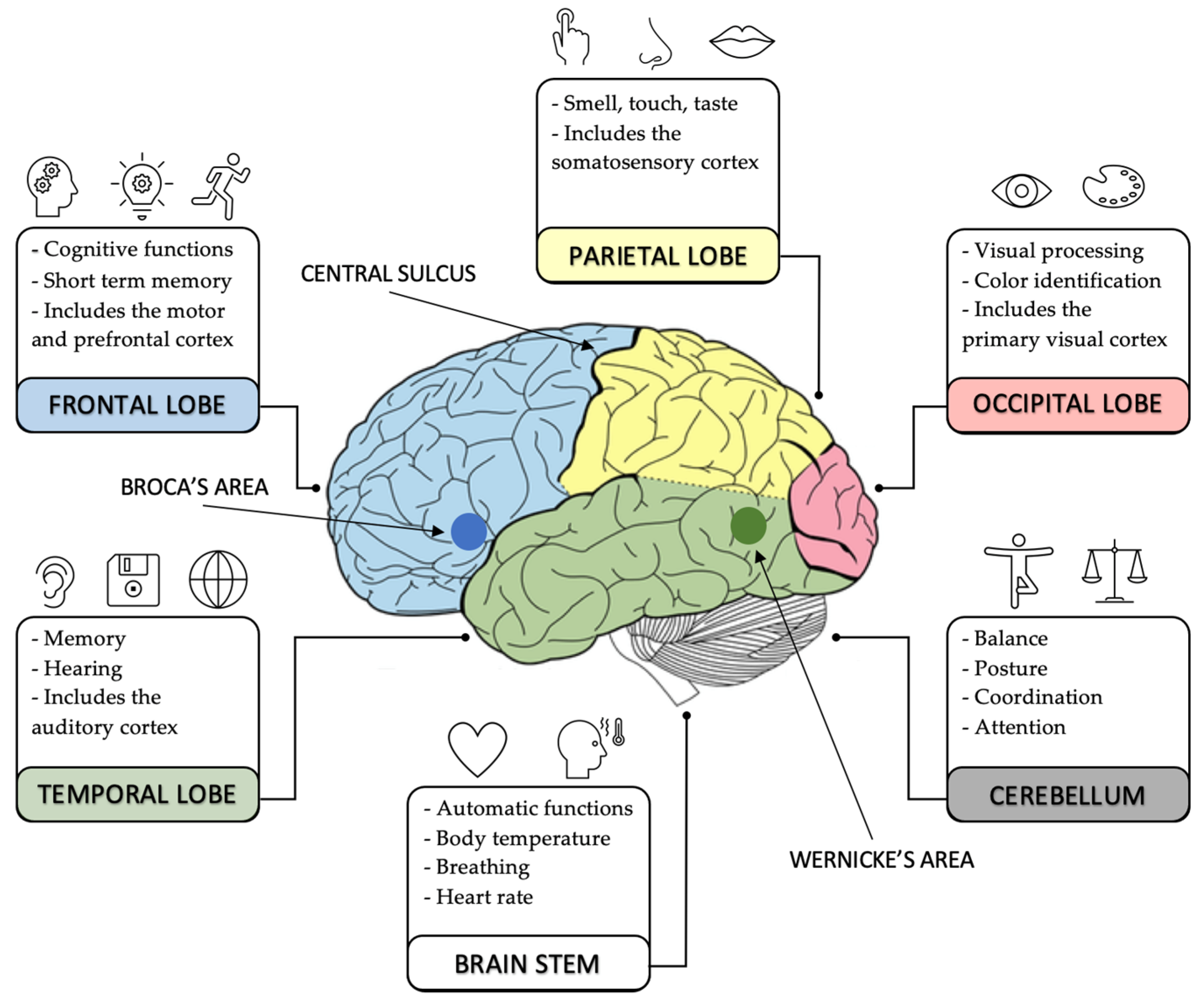
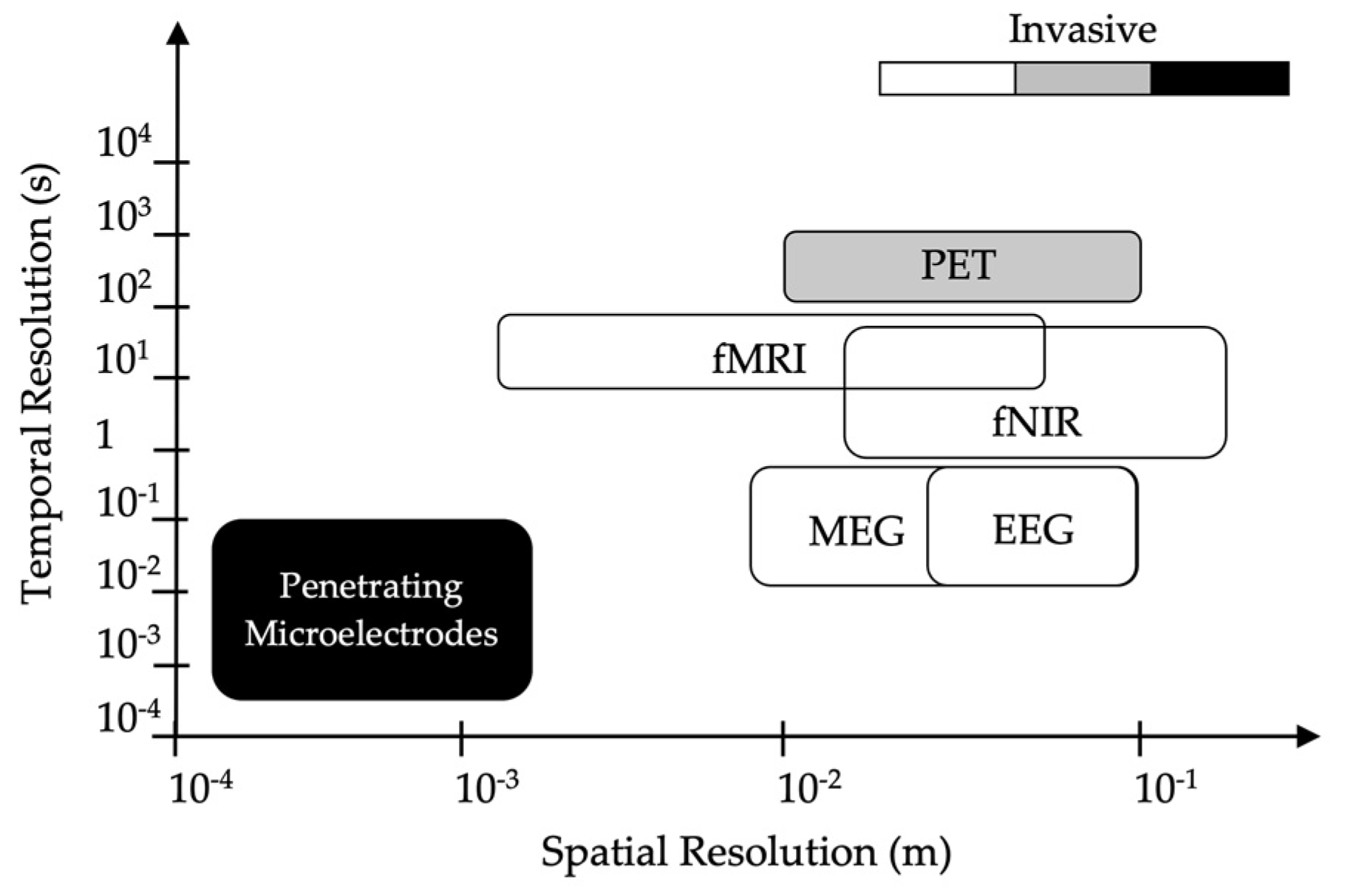
2. Brain and EEG Signal Acquisition

The brain is composed of the cerebrum, cerebellum, and brainstem. More specifically, the cerebrum has two hemispheres, the left and the right hemisphere, which perform higher functions, such as vision, touch, hearing, as well as learning and reasoning, [19,20,21,22]. On the other hand, the cerebellum is underneath the cerebrum and its tasks are to control balance and posture. The brainstem acts as a relay center, connecting the cerebrum and cerebellum to the spinal cord. It accomplishes automatic functions, such as sleep cycles, digestion, and breathing, to name a few. Both hemispheres are joined by a group of fibers called the corpus callosum that communicates between one side and the other. The right hemisphere is related to spatial orientation, non-verbal expression, feelings, creativity, intuition, emotions, and artistic manifestations. The left hemisphere, which is more complex, is mainly related to oral and verbal expression, symbols, the abstract, logic and science.
In addition, the hemispheres are divided into four lobes, i.e., frontal, parietal, temporal, and occipital, as shown in Figure 2. Again, the lobes are divided into areas that perform precise functions. The brain does not function independently, and there are many complex relationships between lobes and between the right and left hemispheres.
The frontal lobe is located in the frontward area of the brain, extending to the central sulcus. It is involved in language, emotion, reasoning, and motor control. The frontal lobe also comprises the motor cortex (involved in movement), the prefrontal cortex (responsible for cognitive functions), and the Broca’s area, located within the left hemisphere (essential for language production). The parietal lobe is situated proximately behind the frontal lobe. It processes data coming from the senses. The parietal lobe holds the somatosensory cortex (necessary for managing sensory information). The temporal lobe is located on the side of the head and it is associated with memory, emotion, hearing, and some aspects of language. The temporal lobe includes the auditory cortex (responsible for processing auditory information) and Wernicke’s area (key for speech comprehension). At last, the occipital lobe is situated in the back zone of the brain and comprises the visual cortex (required for visual data).
In principle, any type of brain signal could be used to provide information about the physiological, functional, and pathological status of the brain, as well as for control. Regarding this last point, brain–computer interfaces (BCI) acquire brain signals and translate them into commands that can carry out desired actions to enhance, replace, restore, or improve human functions. Important advanced BCI research programs and projects have been encouraged by new understanding of brain functions, through the development of powerful low-cost computer equipment. These projects, e.g., Neuralink [24], OpenBCI [25], or Tobii [26], concentrate on developing new augmentative communication and control technology. For instance, Neuralink is creating the future of brain interfaces, developing fully implanted devices that will help people with paralysis. OpenBCI is an open-source brain–computer interface platform working on hardware boards that can be used to measure and record electrical activity produced by the brain that is compatible with standard EEG electrodes. Tobii creates new insights into human behavior and intuitive user interfaces with eye tracking.
Brain control and monitoring is possible due to the small voltage waves and impulses that can be measured and monitored by means of different techniques. Presently, numerous invasive and noninvasive recordings methodologies are employed to store large amounts of images and signals [26,27,28,29,30], summarized in Table 1. In general, numerous complementary approaches are available for recording and imaging the patterns of the brain, such as magnetic, electrical, neuroimaging, and brain stimulations recordings.
Invasive technologies are significantly less susceptible to artifacts, and have higher voltage amplitudes and resolution. In addition, invasive measurement techniques where electrodes are implanted deep in the brain can allow the recording of individual neurons. Arrays of electrodes provide measurements from multiple neurons, increasing the spatial resolution, giving associated data conversely to single recordings. However, invasive recording technologies present risks of surgery and are invasive for patients. Alternatively, several noninvasive recording technologies, where surface electrodes are placed on the scalp are employed, have also been proposed. In this particular case, information acquired present a higher degree of external interference and artifacts (such as 50-Hz power distribution, eye movements, facial movements, briefing, chewing, swallowing, etc.), but measurements do not require surgery. In addition, surface recordings provide high temporal resolutions (on the order of milliseconds) and complete descriptions of the anatomy and physiology of underlying brain structures. Due to interference and the low amplitude in the acquired signals, it is important to augment neural activity.
More specifically, electric recordings are based on measurements of electric fields (and therefore associated electric currents) emanating from active populations of neurons that happen in the brain during its activity. These electronic recordings include different precise methods, making use of electrodes, like in electroencephalography (EEG) (where the electrodes are positioned on the surface of the scalp), electrocorticography (ECoG) (where the implanted electrodes are positioned on the upper layers of cerebral cortex), local field potential (LFP) (where arrays of electrodes are positioned inside the brain), and single unit recordings or spikes (where arrays of microelectrodes are inserted close to neurons). Concerning magnetic recordings, the magnetoencephalography (MEG) technique is usually used, and it measures the magnetic field induced by electrical activity in the brain. Among noninvasive technologies, imaging methods analyze metabolic changes. The activation of neurons requires oxygen, which is absorbed from surrounding blood vessels. As a consequence, this higher level of oxygen is detected and represented. The blood flow and uptake of oxygen by neurons is relatively slow, on the order of seconds. Hence, this method offers good spatial resolution but a very reduced temporal resolution. The commonly used imaging methods can be defined as functional near-infrared recordings (fNIR) (this method measures near-infrared light absorbance of hemoglobin), functional magnetic resonance imaging (fMRI) (this method detects the variations in oxygenated and deoxygenated hemoglobin in the blood), and positron emission tomography (PET) (this method identifies radioactive substances due to the metabolic activity caused by the brain).
In addition to previous neural recording technologies, neural stimulation technologies can be used. In this case, a specific region of the brain is excited by means of an external electrical or magnetic stimulation to obtain a desired brain response. It is worthwhile to mention that recording electrodes can also be employed for stimulations. The techniques used in brain stimulations are transcranial magnetic stimulation (TMS) (this method is based on the magnetic field changes of a coil situated next to the skull), transcranial direct current stimulation (tDCS) (this method excites precise portions of the brain by means of small currents), and deep brain stimulation (DBS) (this method uses electrodes fixed in specific brain areas). Depending on the target application, temporal and spatial resolutions require different acquisition techniques, as can be seen in Figure 3.
More precisely, penetrating electrodes used in brain stimulation have the highest spatial and temporal resolutions, but the invasive nature of this technique reduces its application to limited number of cases. Regarding non-invasive techniques, EEG and MEG have one of the highest temporal resolutions with spatial resolutions of the order of centimeters. On the other hand, fMRI has the highest spatial resolution compared to EEG and MEG; nonetheless, it possesses lower temporal resolution. Finally, fNIR and PET present the lowest spatial and temporal resolutions, respectively.
In practice, EEG is one of the most commonly used methods for capturing neural signals compared to other techniques, as it provides low costs, simplicity, tolerance to motion from subjects, and no radiation exposure risks (the only disadvantages are related to its low spatial resolution or poor signal-to-noise ratio). It was proposed in 1927 by Hans Berger, who defined EEG as a technique for functional exploration the central nervous system by means of recording the brain’s electrical activity in real time [31]. In order to record and store the electrical activity of the brain, the subject wears an EEG cap on top of the head, which requires regular spatial location of electrodes on the scalp for capturing this electrical activity in the form of waves. The 10-20 EEG placement system is an internationally recognized method (by the International Federation of Societies for Electroencephalography and Clinical Neurophysiology or the American EEG Society) employed for this purpose, and is shown in Figure 4.
The 10–20 system settings specify a constant distance of 20% and 10% between electrodes (21 electrodes in total, excluding the earlobe electrodes) by using specific anatomic landmarks. In addition, the odd electrodes are on the left side and the even ones are on the right side. In order to set a larger number of electrodes, the 10–20 system settings recommend placing the rest of the electrodes equidistantly. In Figure 4c, the locations of the 75 electrodes, counting the reference electrodes established by the American EEG Society, can be observed.
The EEG signals obtained during measurements are normally divided into frequency bands, see Figure 4d. Mainly, based on the frequency band and signal amplitude, five major brain waves can be distinguished. First, the delta band is the slowest wave with the highest amplitude (between 20 and 200 μV), lying within the frequency range of 0.5 to 4 Hz. It is related with deep sleep and can also appear in a waking state. Theta waves are within the range of 4 to 7.5 Hz, have relatively high amplitude (>20 μV) and are mainly to signifying drowsiness in young children or arousal in adults. These waves are also related to creative inspiration and deep meditation.
Alpha waves are normally located in the occipital region, but can be present in posterior lobes. These waves present frequencies in the range of 8 to 13 Hz, have low to moderate amplitudes (between 30 and 50 μV) and commonly appears as a round- or sinusoidal-shaped signal. This brain rhythm can be associated with relaxed awareness without any attention or concentration. Finally, beta waves present frequencies within the range of 14 to 26 Hz (sometimes higher frequencies are mentioned) with small amplitudes (between 5 and 30 μV). These waves are generated principally over the frontal and central regions of the brain and can be associated with thinking. Frequencies exceeding 30 Hz (mainly up to 45 Hz) correspond to the gamma band (occasionally designated as fast beta waves) characterized by their tiny amplitudes (<5 μV).
The identification and understanding of the aforementioned brain rhythms obtained from measured EEG signals are not trivial (the nature of EEG signals is highly non-linear, non-Gaussian, random, and non-correlated). Therefore, in many cases, advanced signal processing tools are used to quantify the information and to help with the identification of brain rhythms and in the diagnosis of brain disorders and impairments. The next section describes the EEG signal processes that are generally employed to obtain complete neurofeedback analyses.

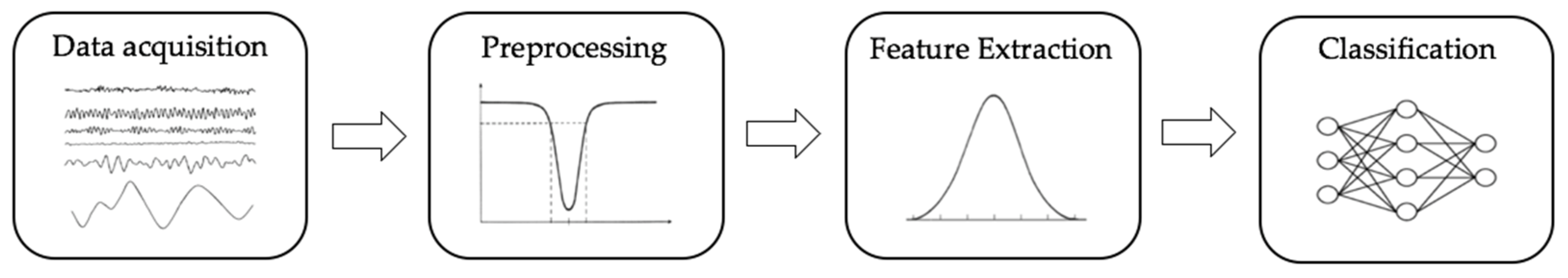
3. EEG Signal Processing

The measured raw EEG signals can contain interference that is divided into system artifacts and patient-related (physiological). The patient-related or internal artifacts are due to body movements, eye-blinking, breathing, or sweating. The system artifacts are due to 50/60 Hz power-feeding interference, electrical noise from the electronic equipment and components, impedance fluctuations of the electrodes, or cable defects. Consequently, it is of key importance to process and retain effective information of EEG signals, removing artifacts and interference with the aim of obtaining clear information for later classification and diagnosis. Different filtering schemes for removing EEG artifacts that are commonly applied to raw EEG signals are summarized in Table 2.
As can be observed, EEG signals are modified using three types of filters. High-pass filters (cut-off frequency below 0.5 Hz) avoid very low frequency interference, like breathing. Low-pass filters (cut-off frequency of approximately 50–70 Hz) can be employed to eliminate high-frequency noise, and Notch filters (at 50/60 Hz) are often necessary to improve rejection of electric power supply artifacts. Once the EEG signal has been preprocessed and cleaned of noise and external interference, it can be finally treated to extract its main properties or features for later classification (see Figure 1).
A feature can be defined as a unique characteristic that allows to understand the neural activity and assess the state of the brain. EEG features depends on various factors, e.g., age, mental state of subject, or sex, to name a few. Thus, and as can be presumed, the underlying dynamics happening in the brain involve many aspects (linear as well as non-linear), which determine these characteristic features. In this regard, several signal processing methods have been proposed to isolate and extract significant features that help to diagnose complex features that can take place.
These signal processing methods are divided in four fundamental domains [33,34,35,36,37,38,39,40], as can be seen in Table 3. Furthermore, various algorithms have been established to visualize brain activity using restructured images from EEGs. Each domain presents advantages and problems, where each technique is optimal depending on the information that one wants to extract.
Temporal analysis permits to identify normal and abnormal wave outlines in the EEG signal, and it is useful to identify the presence or absence of brain rhythms. In general, EEG signals are often correlated in time. Consequently, time samples can be estimated employing previous samples by means of autoregressive models (for stationary signals) or adaptive autoregressive models (for nonstationary signals), such as linear prediction (LP) and independent component analysis (ICA). The main features that can be obtained from the latter classification are event related potentials (ERP), statistics of signal power (mean, standard deviation, 1st difference, 2nd difference, entropy), Hjorth features (activity, mobility, complexity), fractal dimension (FD), and high order crossings (HOC).
In some cases, temporal methods cannot provide significant features. This can happen due to poor temporal or spatial resolutions in a recorded signal, where only oscillatory activity could be captured. Theoretically, these oscillations may be represented by basic sinusoid functions making use of the Fourier transform (FT). In these cases, spectral analysis gives additional information, resolving the dominant frequencies present in the EGG signal. The main methods employed in this case are fast Fourier transform (FFT), short-time Fourier transform (STFT), spectrogram, autoregressive method (ARM), and Eigenvectors, where the main features that are extracted are band power and high order spectra (HOS). Typically, for neuronal signals, short-time Fourier transform (STFT) or spectrograms offer better results as short-time windows are employed by dividing the data into small time intervals.
The benefits of temporal and frequency studies can be combined to obtain improved EEG studies. For nonperiodic signals, time-frequency transformations are usually applied for signal decomposition, providing a great deal of important information. Signals can be decomposed into single instantaneous frequencies over time by applying different methods, i.e., Wigner–Ville distribution, scalogram, Hilbert–Huang spectrum or discrete wavelet transform (DWT). The advantage of this method is that non-linear, nonstationary neural information can be converted into linear and stationary components. In addition, this technique allows to obtain a compromise between time and frequency resolutions to have an optimum representation of the signals.
Finally, spatial-time-frequency analysis estimates the distribution of brain rhythms and characteristic features over different brain regions. Spatial referencing methods can be useful to augment local activity, filtering the noise measured from different electrodes and approximate the variance of the EEG information.

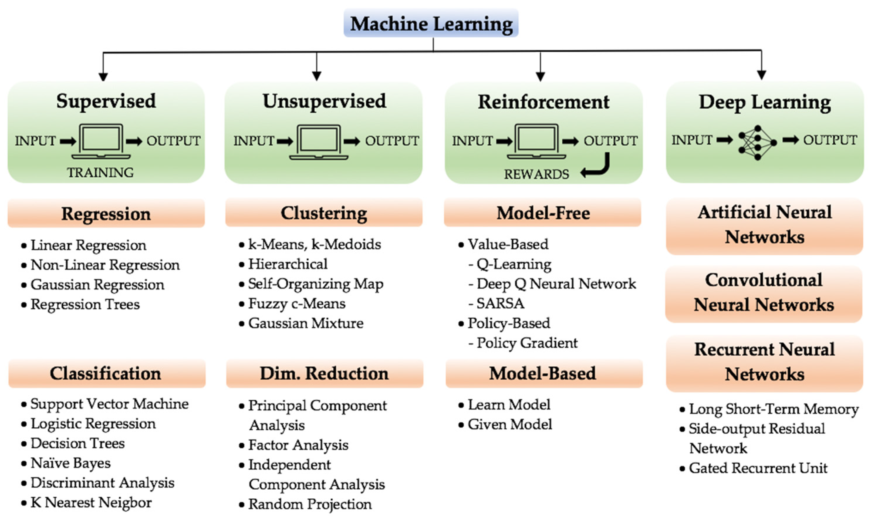
4. Machine Learning Algorithms Employed in EEG Signal Classification

This section provides a concise description of machine learning methods used in EEG analysis for classification. Once feature extraction is successfully carried out, the processed EEG data are finally ready for classification by means of machine learning algorithms.
Machine learning can be defined as computer models and algorithms that are able to automatically learn and adapt from data and experience without explicit instructions or human intervention [41,42,43,44,45,46,47,48]. As can be seen in Figure 5, machine learning methods can be classified into four categories: supervised learning, unsupervised learning deep learning, and reinforcement learning— the first three being more common.
Supervised learning algorithms utilize predefined inputs and known outputs to construct a model using data points with known outcomes. Thereafter, the system is able to make decisions or predictions (predict forthcoming outputs using new data) from the acquired training and experience. Supervised learning can be divided into two categories i.e., regression and classification. Representative regression learning algorithms are linear regression, non-linear regression, Gaussian process regression, and regression trees, generally used for the prediction of continuous variables. Classification algorithms like support vector machines (SVM), logistic regression, decision trees, naïve Bayes, discriminant analysis, and k nearest neighbor (kNN) are employed for categorical output variables; only two classes of values are possible, such as yes–no, male–female, true–false, etc.
On the contrary, in unsupervised learning, algorithms involve only input datasets but no outputs, inferring the outcome patterns without any reference, so that the machine does not need any external supervision to learn from the data. This method is classified into clustering and dimensionality reduction. Clustering algorithms, such K-means, k-medoids, hierarchical clustering, self-organizing map, fuzzy c-means and Gaussian mixture, typically match the input data that presents similarities into clusters and categorizes them according to the presence or absence of those similarities. Dimensionality reduction is obtained by reducing the number of input variables in a dataset to simplify the classification and better fit a predictive model while minimizing the loss of information; for instance, principal component analysis, factor analysis, independent component analysis, and random projection. Unsupervised learning can carry out more complex tasks than supervised learning, but it is essentially more difficult to implement.
In reinforcement learning, the employed algorithms learn from their own experiences; an agent learns from an unidentified environment to achieve a purpose. That is, the algorithms are capable of making the best decision according to a procedure in which the correct decisions are rewarded. The main elements of a reinforcement learning system are the agent, the environment, the action, the policy and the reward. The agent is the program that is trained with the objective of achieving a specific task. The environment is the world, real or virtual, in which the agent executes actions. The action is a change made by an agent that modifies the status of the environment and the policy are the criterions that the agent follows when making actions. The reward is the evaluation of an action that can be positive or negative. Reinforcement learning procedures are classified as model-free and model-based algorithms. Model-free algorithms do not construct an explicit model of the environment, but rather runs actions with the environment to directly derive the optimal policy, similar to trial-and-error algorithms. Model-free algorithms are either value-based or policy-based, where value-based algorithms (like Q-learning, deep Q neural network (DQN) and state-action-reward-state-action (SARSA)) reflect an optimal strategy as a result of exactly guessing the value function in every state. Policy-based algorithms (like policy gradient) evaluate the optimal policy without modeling the value function. Model-based algorithms (like learn/given model) construct a concrete model of the environment and the agent explores that environment to learn it. For each state and action, the model estimates the expected reward and the future state.
At last, it is worthwhile to highlight a specific subset of machine learning algorithms, known as deep learning, due to their interesting characteristics [14,49]. Deep learning is mainly based on multi-layered (input, hidden and output layers) neural networks that learn from large amounts of data, emulating the functions and workings of the human brain, computing information using millions of neurons. The input layer has input features of the dataset introduced to the neural network. The hidden layers, that can vary from a few to several layers depending on the complexity of the problem to solve, are placed between input layers and output layers and each layer creates an output from a set of weighted inputs. The output layer produces the final results for given inputs. In this way, deep learning algorithms repeatedly perform calculations and predictions in each layer, progressively learning and gradually improving the accuracy of the results over time. Commonly, deep learning can be categorized into three types of algorithms, i.e., artificial neural networks (ANN), convolutional neural networks (CNN), and recurrent neural networks (RNN). Artificial neural networks (ANNs), also known as simulated neural networks (SNNs), are the core of deep learning algorithms and their structure is inspired by the human brain, simulating the behavior of biological neurons. ANNs are capable of learning any nonlinear function, based on an activation function that helps the network to learn any complex relationship between inputs and outputs. These networks are also widely known as universal function approximators. CNNs (or ConvNets) are neural networks mainly used for auto-correlated data processing. The basic element of CNNs are filters, also known as kernels, employed to acquire relevant features from the input by means of convolutional operations. CNNs generally present several specialized hidden layers showing different functions and hierarchies, i.e., first hidden layers can detect simple patterns, the next layers can identify patterns, and the final hidden layers are specialized and can recognize complex patterns. RNNs are neural networks that have recurrent connections between hidden layers. This recurrent feedback ensures that sequential information is captured in the input data. Therefore, RNNs can normally be used in problems related to time series data. The most employed algorithms to develop RNNs are long short-term memory (LSTM), side-output residual network (SRN) and gated recurrent unit (GRU).
The main difference between deep and machine is how data is processed and how algorithms learn from them. While all machine learning procedures can work and learn from structured and tagged data, deep learning can also process unstructured and unlabeled data. Rather than relying on labels within the data to identify and classify objects and information, deep learning uses a multi-layered neural network to extract characteristics from the data and increasingly improve the identification and classification of the data itself. Table 4 summarizes the main differences between both classification approaches, where several properties, i.e., data format, database size, training, algorithm, and applications, are analyzed. Finally, deep learning models are also capable of reinforcing learning, which is a more advanced unsupervised learning process in which the model “learns” to be more accurate based on positive feedback from previous calculations.
Next, in Table 5, a summary of the most known algorithms employed in machine learning is shown. The main characteristics of each algorithm, as well as the advantages and disadvantages of the methods, are also presented in the table.
It can be concluded that supervised learning views output values based on the received training. Unsupervised learning groups together data depending on similarity and creates clusters. Reinforcement learning, which is a subgroup of unsupervised learning, completes learning differently, and it employs a method of cause and effect by means of rewards. Deep learning techniques are particularly well-suited for complex data classifications tasks and, thus, are particularly well-suited to solve problems related to brain signals.
Current machine learning classification methods used in EEG applications have shown that supervised algorithms, either regression or classification, such naïve Bayes, decision tree, KNN or SVM are on average of higher accuracy than their unsupervised counterparts. In addition, individually applied methods are limited in their accuracy but, the combination of methods when implemented properly, can have higher overall classification accuracy. Concerning deep learning, it has recently shown notable results and progress across EEG signals, such as patient classification, diseases diagnosis, or patient treatment [49,50,51,52]. However, some challenges remain, for instance the vanishing gradient in ANN, such as in networks with a large number of hidden layers; the weights of a neural network (updated finding gradients) vanish as it propagates through the layers. Consequently, ANNs cannot capture sequential information in the input data. In the case of RNNs, they also suffer from the vanishing gradient drawback.
Furthermore, other general problems detected in the revised research are mainly related to small datasheets that were recorded or few existing relevant data in datasheets. As is well known, the quality and amount of data are of primary importance in machine learning. Different approaches can be used to improve predictive models from small datasets. The use of simple classifier models like naïve Bayes, regression models, short decision trees is less susceptible to overfitting as they essentially are trying to learn less. Additionally, the use of ensemble methods, where the decisions between classifiers can compensate for learning.
In the particular case of few existing relevant data in datasheets, transfer learning [53,54,55,56], data augmentation [57,58,59,60], or synthetic data [61,62,63,64] techniques are usually applied to generate improved machine learning training and models. Transfer learning is based on the knowledge acquired from another existing learned task to improve the performance of a new machine learning model; thus, reducing the amount of required training data. Simply combining different datasets may not always improve input data if the existing datasets are different from the target data as the new model would be trained inaccurately. In addition, the lack of quality labeled data can be overcome through transfer learning. Data augmentation is based on an increase in representative data. By these means, the prediction accuracy of the model can be improved as training data is increased, overfitting is reduced, and scarcity is prevented. Some of the most common data augmentation techniques used in practice are the generative adversarial networks (GAN) employed to generate new data samples or neural style transfer (NST) used to combine datasets. The GAN method divides its main algorithm into two sub-models, the generator model and the discriminator model. Both models are trained together by means of a zero-sum game. Finally, synthetic data, on the contrary, generate new false data that have equivalent representation and statistical properties of its real counterpart. Particularly, synthetic minority over-sampling technique (SMOTE) and modified-SMOTE are the most used techniques.
In summary, the presented results prove that machine learning can successfully implement practical complementarity for enhanced feature extraction and classification, especially in EEG signal analysis. More specifically, these results show that deep learning provides a significant breakthrough in the classification of EEG data, outperforming, in many cases, traditional machine learning methods. In addition, a great deal of work should be carried out in many new research areas, such as autobiographical memory.

5. EEG Neurofeedback in Autobiographical Memory Analyses

Recent advances in signal processing and machine learning, as well as improvements in the ability to collect, store, and process massive amounts of data, have provided significant progress and new insights into neurological computerized analysis. EEG signals are intrinsically complex with non-Gaussian, non-stationary, and often non-linear natures. Therefore, the help of both signal processing and machine learning offers the possibility to obtain objective clinical diseases diagnoses, predictions, and the monitoring of treatment (in addition to the subjective interpretation of EEG recordings). Significant uses of EEGs in neural studies have been applied to a variety of brain disorders, i.e., Parkinson disease, epilepsy, tremor, strokes, concussions, bipolar disorder, schizophrenia, depression, and sleep disorders, to name a few, or they have simply been applied to brain monitoring or brain rhythms detection. Concerning autobiographical memory deficits in schizophrenia evaluated through EEG, in order to rigorously identify previous publications to date a preferred reporting items for systematic reviews and meta-analyses (PRISMA) analysis has been performed and is shown in Figure 6.
The articles included in the analysis are summarized in Table 6, which provides an overview and comparison of the most significant published research papers. Particularly, the assigned reference, the signal processing carried out and the conclusions obtained are listed.
As can be readily observed in several assertions obtained within the research papers presented in Table 5, memory access mainly implies the usage of frontal and temporal regions of the brain. Therefore, the delta rhythm is mostly involved in the memory endeavor (as it is interrelated with the frontal lobe) but theta and gamma rhythms can also be affected to a lesser extent. In addition, emotional disorders and schizophrenia generally yield difficulties to memory access, and these difficulties could be reduced by means of psychotherapeutic treatment. Lastly, most studies presented to date have made use of neuroimaging (it detects areas that are activated) rather than EEG (that indicates interconnections between brain areas), and the acquired signals have been processed employing the techniques described in Table 3 and Table 5, but machine learning is still lacking in most of the analyses performed.
Deeper and more complete studies should be carried out in the specific research area of autobiographical memory, in particular as related to brain disorders, such schizophrenia, to provide better insights of the underlying processes that could explain psycopathological impairments in the brain. It will give answer to issues such as differences in memory retrieval connections between controls and patients suffering from schizophrenia, what areas are activated and connected to each other in specific memories needed to improve social functioning and adaptation, differences depending on whether the memory is specific or overgeneral and dysfunctional, the role of depressive symptoms in the specificity of auto-biographical memory transdiagnostically, or differences depending on whether the memory is emotionally positive or negative (within patients with schizophrenia and/or depressive signs). The answer to these and similar questions, and the application of machine learning and new signal processing methods can provide great advances in the neurofeedback of autobiographical memory and treatment of its impairment.

6. Conclusions

In this paper, the structure of the brain and methods used for signal acquisition are presented. After the general introduction, the paper focuses on EEG techniques and associated signal processing. EEG analyses can be divided into signal acquisition, preprocessing, feature extraction, and classification (usually using simple inspection methods or more complex procedures such as machine learning). Concerning signal acquisition, it is usually obtained with EEG nets following the internationally recognized 10–20 EEG placement criteria. Next, signal preprocessing permits to remove external artifacts due to power supply interference, electrical noise from the electronic equipment and components, impedance fluctuation of the electrodes, or cable defects. On the other hand, feature extraction methods are typically performed in time, frequency, or space domains and classification is carried out by applying machine learning algorithms classified as supervised, unsupervised, reinforcement systems, or deep learning. In this regard, developments in machine learning have notably increased the possibility of performing reliable diagnoses of neurological impairments and disorders. Especially, deep learning algorithms provide the best classification and understanding of brain signals. However, problems related to small datasheets or few relevant data points in datasheets have to be improved.
Finally, research devoted to neurofeedback in autobiographical memory to date shows that patients with brain disorders, e.g., depression or schizophrenia, have difficulty accessing memory-related areas of the brain. Mainly, the frontal and temporal lobes, and the delta rhythm are affected during memory retrieval. Nevertheless, research associated with autobiographical memory has to yet answer key intrinsic aspects of brain functioning and therefore a great deal of research efforts remains necessary in this area. Thus, machine learning insights could show and improve processes involved in the recovery of the specificity of autobiographical memory, which is undermined under clinical diagnoses, such as schizophrenia.

Author Contributions

The contributions of authors are: Conceptualization, M.Á.L., M.V.J., J.M.S., J.J.R. and A.L.B.; methodology, M.Á.L., M.V.J., J.M.S., J.J.R. and A.L.B.; software, M.Á.L., J.M.S. and A.L.B.; validation, M.Á.L., M.V.J., J.M.S., J.J.R. and A.L.B.; formal analysis, M.Á.L., M.V.J., J.M.S., J.J.R. and A.L.B.; investigation, M.Á.L., J.M.S. and A.L.B.; resources, M.Á.L., M.V.J., J.M.S., J.J.R. and A.L.B.; writing—original draft preparation, M.Á.L. and A.L.B.; writing—review and editing, M.Á.L. and A.L.B.; visualization, M.Á.L., M.V.J., J.M.S., J.J.R. and A.L.B.; supervision, J.M.S., J.J.R. and A.L.B.; project administration, J.M.S. and A.L.B.; funding acquisition, J.M.S., J.J.R. and A.L.B. All authors have read and agreed to the published version of the manuscript.

Funding

This work was supported by the Castilla-La Mancha Department of Education, Culture and Sports and the European Regional Development Fund under SPBLY/19/180501/000181 grant and the Spanish Ministerio de Ciencia, Innovación y Universidades (Spain) under PID2019-103956RB-I00 grant.

Conflicts of Interest

The authors declare no conflict of interest.

References

  1. Meziani, A.; Djouani, K.; Medkour, T.; Chibani, A. A Lasso quantile periodogram based feature extraction for EEG-based motor imagery. J. Neurosci. Methods 2019, 328, 108434. [Google Scholar] [CrossRef]
  2. von Bunau, P.; Meinecke, F.C.; Scholler, S.; Muller, K.R. Finding stationary brain sources in EEG data. In Proceedings of the 32nd Annual International Conference of the IEEE Engineering in Medicine and Biology Society, Buenos Aire, Argentina, 30 August–4 September 2010; pp. 2810–2813. [Google Scholar] [CrossRef]
  3. Feyissa, A.M.; Tatum, W.O. Adult EEG. Handb. Clin. Neurol. 2019, 160, 103–124. [Google Scholar] [CrossRef]
  4. Micoulaud-Franchi, J.A.; McGonigal, A.; Lopez, R.; Daudet, C.; Kotwas, I.; Bartolomei, F. Electroencephalographic neurofeedback: Level of evidence in mental and brain disorders and suggestions for good clinical practice. Neurophysiol. Clin. 2015, 45, 423–433. [Google Scholar] [CrossRef] [PubMed]
  5. Ahmadlou, M.; Adeli, H. Functional community analysis of brain: A new approach for EEG-based investigation of the brain pathology. Neuroimage 2011, 58, 401–408. [Google Scholar] [CrossRef]
  6. Nicolas-Alonso, L.F.; Gomez-Gil, J. Brain computer interfaces, a review. Sensors 2012, 12, 121112–121179. [Google Scholar] [CrossRef] [PubMed]
  7. Huster, R.J.; Calhoun, V.D. Progress in EEG: Multi-subject Decomposition and Other Advanced Signal Processing Approaches. Brain Topogr. 2018, 31, 1–2. [Google Scholar] [CrossRef] [PubMed] [Green Version]
  8. Urigüen, J.A.; Garcia-Zapirain, B. EEG artifact removal-state-of-the-art and guidelines. J. Neural Eng. 2015, 12, 031001. [Google Scholar] [CrossRef]
  9. Jiang, X.; Bian, G.B.; Tian, Z. Removal of Artifacts from EEG Signals: A Review. Sensors 2019, 19, 987. [Google Scholar] [CrossRef] [PubMed] [Green Version]
  10. Ai, Q.; Chen, A.; Chen, K.; Liu, Q.; Zhou, T.; Xin, S.; Ji, Z. Feature extraction of four-class motor imagery EEG signals based on functional brain network. J. Neural Eng. 2019, 16, 026032. [Google Scholar] [CrossRef]
  11. Khademi, A.; Reiche, B.; DiGregorio, J.; Arezza, G.; Moody, A.R. Whole volume brain extraction for multi-centre, multi-disease FLAIR MRI datasets. Magn. Reson. Imaging 2020, 66, 116–130. [Google Scholar] [CrossRef] [Green Version]
  12. Hira, Z.M.; Gillies, D.F. A Review of feature selection and feature extraction methods applied on microarray data. Adv. Bioinform. 2015, 2015, 198363. [Google Scholar] [CrossRef]
  13. Ker, J.; Bai, Y.; Lee, H.Y.; Rao, J.; Wang, L. Automated brain histology classification using machine learning. J. Clin. Neurosci. 2019, 66, 239–245. [Google Scholar] [CrossRef]
  14. Craik, A.; He, Y.; Contreras-Vidal, J.L. Deep learning for electroencephalogram (EEG) classification tasks: A review. J. Neural Eng. 2019, 16, 031001. [Google Scholar] [CrossRef] [PubMed]
  15. Burgos, N.; Colliot, O. Machine learning for classification and prediction of brain diseases: Recent advances and upcoming challenges. Curr. Opin. Neurol. 2020, 33, 439–450. [Google Scholar] [CrossRef] [PubMed]
  16. Gao, S.; Calhoun, V.D.; Sui, J. Machine learning in major depression: From classification to treatment outcome prediction. CNS Neurosci. Ther. 2018, 24, 1037–1052. [Google Scholar] [CrossRef] [PubMed] [Green Version]
  17. Vanegas, M.I.; Blangero, A.; Galvin, J.E.; Di Rocco, A.; Quartarone, A.; Ghilardi, M.F.; Kelly, S.P. Altered dynamics of visual contextual interactions in Parkinson’s disease. NPJ Parkinsons Dis. 2019, 5, 13. [Google Scholar] [CrossRef] [Green Version]
  18. Vanegas, M.I.; Ghilardi, M.F.; Kelly, S.P.; Blangero, A. Machine learning for EEG-based biomarkers in Parkinson’s disease. In Proceedings of the BIBM 2018: 2018 IEEE International Conference on Bioinformatics and Biomedicine (BIBM18), Madrid, Spain, 3–6 December 2018; pp. 2661–2665. [Google Scholar] [CrossRef]
  19. Casillo, S.M.; Luy, D.D.; Goldschmidt, E. A History of the Lobes of the Brain. World Neurosurg. 2020, 134, 353–360. [Google Scholar] [CrossRef]
  20. Caserta, M.T.; Bannon, Y.; Fernandez, F.; Giunta, B.; Schoenberg, M.R.; Tan, J. Normal brain aging clinical, immunological, neuropsychological, and neuroimaging features. Int. Rev. Neurobiol. 2009, 84, 1–19. [Google Scholar] [CrossRef]
  21. Hernández-Peón, R.; Sterman, M.B. Brain functions. Annu. Rev. Psychol. 1966, 17, 363–394. [Google Scholar] [CrossRef]
  22. Horn, A.; Ostwald, D.; Reisert, M.; Blankenburg, F. The structural-functional connectome and the default mode network of the human brain. Neuroimage 2014, 102, 142–151. [Google Scholar] [CrossRef]
  23. Wikipedia. File: Lobes of the Brain NL.svg. 2021. Available online: https://es.m.wikipedia.org/wiki/Archivo:Lobes_of_the_brain_NL.svg (accessed on 17 November 2021).
  24. Neuralink. 2016. Available online: https://neuralink.com (accessed on 17 November 2021).
  25. OpenBCI. 2014. Available online: https://openbci.com (accessed on 17 November 2021).
  26. Tobii. 2001. Available online: https://www.tobii.com (accessed on 17 November 2021).
  27. Koch, G.; Caltagirone, C. Non-invasive brain stimulation: From brain physiology to clinical opportunity. Neurosci. Lett. 2020, 719, 134496. [Google Scholar] [CrossRef]
  28. Nardone, R.; Höller, Y.; Leis, S.; Höller, P.; Thon, N.; Thomschewski, A.; Golaszewski, S.; Brigo, F.; Trinka, E. Invasive and non-invasive brain stimulation for treatment of neuropathic pain in patients with spinal cord injury: A review. J. Spinal Cord Med. 2014, 37, 19–31. [Google Scholar] [CrossRef] [PubMed] [Green Version]
  29. Solomons, C.D.; Shanmugasundaram, V. A review of transcranial electrical stimulation methods in stroke rehabilitation. Neurol. India 2019, 67, 417–423. [Google Scholar] [CrossRef]
  30. Biasiucci, A.; Franceschiello, B.; Murray, M.M. Electroencephalography. Curr. Biol. 2019, 29, R80–R85. [Google Scholar] [CrossRef] [Green Version]
  31. Berger, H. Über das elektroenkephalogramm des menschen. Eur. Arch. Psychiatry Clin. Neurosci. 1929, 87, 527–570. [Google Scholar] [CrossRef]
  32. Saeid, S.; Chambers, J.A. EEG Signal Processing; John Wiley & Sons: Chichester, UK, 2007. [Google Scholar] [CrossRef]
  33. Durongbhan, P.; Zhao, Y.; Chen, L.; Zis, P.; De Marco, M.; Unwin, Z.C.; Venneri, A.; He, X.; Li, S.; Zhao, Y.; et al. A Dementia Classification Framework Using Frequency and Time-Frequency Features Based on EEG Signals. IEEE Trans. Neural Syst. Rehabilit. Eng. 2019, 27, 826–835. [Google Scholar] [CrossRef] [PubMed] [Green Version]
  34. Miwakeichi, F.; Martínez-Montes, E.; Valdés-Sosa, P.A.; Nishiyama, N.; Mizuhara, H.; Yamaguchi, Y. Decomposing EEG data into space-time-frequency components using Parallel Factor Analysis. Neuroimage 2004, 22, 1035–1045. [Google Scholar] [CrossRef]
  35. Sun, Y.; Zhang, G.; Zhang, X.; Yan, X.; Li, L.; Xu, C.; Yu, T.; Liu, C.; Zhu, Y.; Lin, Y.; et al. Time-frequency analysis of intracranial EEG in patients with myoclonic seizures. Brain Res. 2016, 1652, 119–126. [Google Scholar] [CrossRef] [PubMed]
  36. Auboiroux, V.; Larzabal, C.; Langar, L.; Rohu, V.; Mishchenko, A.; Arizumi, N.; Labyt, E.; Benabid, A.L.; Aksenova, T. Space-Time-Frequency Multi-Sensor Analysis for Motor Cortex Localization Using Magnetoencephalography. Sensors 2020, 20, 2706. [Google Scholar] [CrossRef]
  37. Khoshnevis, S.A.; Sankar, R. Applications of higher order statistics in electroencephalography signal processing: A comprehensive survey. IEEE Rev. Biomed. Eng. 2020, 13, 169–183. [Google Scholar] [CrossRef]
  38. Olias, J.; Martín-Clemente, R.; Sarmiento-Vega, M.A.; Cruces, S. EEG signal processing in mi-BCI applications with improved covariance matrix estimators. IEEE Trans. Neural Syst. Rehabilit. Eng. 2019, 27, 895–904. [Google Scholar] [CrossRef]
  39. Massana, J.; Raya, O.; Gauchola, J.; Lopez, B. SignalEEG A practical tool for EEG signal data mining. Neuroinformatics 2021, 19, 567–583. [Google Scholar] [CrossRef]
  40. McIntosh, J.R.; Sajda, P. Estimation of phase in EEG rhythms for real-time applications. J. Neural Eng. 2020, 17, 034002. [Google Scholar] [CrossRef] [Green Version]
  41. Lv, H.; Tang, H. Machine Learning Methods and Their Application Research. In Proceedings of the 2nd International Symposium on Intelligence Information Processing and Trusted Computing, Wuhan, China, 22–23 October 2011; pp. 108–110. [Google Scholar] [CrossRef]
  42. Wang, H.; Ma, C.; Zhou, L. A Brief Review of Machine Learning and Its Application. In Proceedings of the International Conference on Information Engineering and Computer Science, Wuhan, China, 19–20 December 2009; pp. 1–4. [Google Scholar] [CrossRef]
  43. Zuo, X.N. A machine learning window into brain waves. Neuroscience 2020, 436, 167–169. [Google Scholar] [CrossRef] [PubMed]
  44. Najafzadeh, H.; Esmaeili, M.; Farhang, S.; Sarbaz, Y.; Rasta, S.H. Automatic classification of schizophrenia patients using resting-state EEG signals. Phys. Eng. Sci. Med. 2021, 44, 855–870. [Google Scholar] [CrossRef] [PubMed]
  45. Barros, C.; Silva, C.A.; Pinheiro, A.P. Advanced EEG-based learning approaches to predict schizophrenia: Promises and pitfalls. Artif. Intell. Med. 2021, 114, 102039. [Google Scholar] [CrossRef] [PubMed]
  46. Vázquez, M.A.; Maghsoudi, A.; Mariño, I.P. An interpretable machine learning method for the detection of schizophrenia using EEG signals. Front. Syst. Neurosci. 2021, 15, 652662. [Google Scholar] [CrossRef]
  47. Mortaga, M.; Brenner, A.; Kutafina, E. Towards interpretable machine learning in EEG analysis. Stud. Health Technol. Inform. 2021, 283, 32–38. [Google Scholar] [CrossRef]
  48. Lourenço, C.S.d.S.; Tjepkema-Cloostermans, M.C.; van Putten, M.J.A.M. Machine learning for detection of interictal epileptiform discharges. Clin. Neurophysiol. 2021, 132, 1433–1443. [Google Scholar] [CrossRef]
  49. Gao, Z.; Dang, W.; Wang, X.; Hong, X.; Hou, L.; Ma, K.; Perc, M. Complex networks and deep learning for EEG signal analysis. Cogn. Neurodynamics 2021, 15, 369–388. [Google Scholar] [CrossRef]
  50. Aslan, Z.; Akin, M.A. Deep learning approach in automated detection of schizophrenia using scalogram images of EEG signals. Phys. Eng. Sci. Med. 2021, 1–14. [Google Scholar] [CrossRef] [PubMed]
  51. Ahmedt-Aristizabal, D.; Fernando, T.; Denman, S.; Robinson, J.E.; Sridharan, S.; Johnston, P.J.; Laurens, K.R.; Fookes, C. Identification of children at risk of schizophrenia via deep learning and EEG responses. IEEE J. Biomed. Health Inform. 2021, 25, 69–76. [Google Scholar] [CrossRef]
  52. Sun, J.; Cao, R.; Zhou, M.; Hussain, W.; Wang, B.; Xue, J.; Xiang, J. A hybrid deep neural network for classification of schizophrenia using EEG Data. Sci. Rep. 2021, 11, 4706. [Google Scholar] [CrossRef] [PubMed]
  53. Jiang, Y.; Wu, D.; Deng, Z.; Qian, P.; Wang, J.; Wang, G.; Chung, F.-L.; Choi, K.-S.; Wang, S. Seizure classification from EEG signals using transfer learning, semi-supervised learning and TSK fuzzy system. IEEE Trans. Neural Syst. Rehabilit. Eng. 2017, 25, 2270–2284. [Google Scholar] [CrossRef]
  54. Li, J.; Qiu, S.; Shen, Y.-Y.; Liu, C.-L.; He, H. Multisource transfer learning for cross-subject EEG emotion recognition. IEEE Trans. Cybern. 2019, 50, 3281–3293. [Google Scholar] [CrossRef]
  55. Wei, C.-S.; Lin, Y.-P.; Wang, Y.-T.; Jung, T.-P.; Bigdely-Shamlo, N.; Lin, C.-T. Selective transfer learning for EEG-based drowsiness detection. In Proceedings of the IEEE International Conference on Systems, Man, and Cybernetics, Kowloon Tong, Hong Kong, 9–12 October 2015; pp. 3229–3232. [Google Scholar] [CrossRef]
  56. Raghu, S.; Sriraam, N.; Temel, Y.; Rao, S.V.; Kubben, P.L. EEG based multi-class seizure type classification using convolutional neural network and transfer learning. Neural Netw. 2020, 124, 202–212. [Google Scholar] [CrossRef]
  57. Luo, Y.; Lu, B.-L. EEG data augmentation for emotion recognition using a conditional Wasserstein GAN. In Proceedings of the 40th Annual International Conference of the IEEE Engineering in Medicine and Biology Society (EMBC), Honolulu, HI, USA, 17–21 July 2018; pp. 2535–2538. [Google Scholar] [CrossRef]
  58. Bird, J.J.; Pritchard, M.; Fratini, A.; Ekárt, A.; Faria, D.R. Synthetic Biological Signals Machine-generated by GPT-2 improve the Classification of EEG and EMG through Data Augmentation. IEEE Robot. Autom. Lett. 2021, 6, 3498–3504. [Google Scholar] [CrossRef]
  59. Lashgari, E.; Liang, D.; Maoz, U. Data augmentation for deep-learning-based electroencephalography. J. Neurosci. Methods 2020, 346, 108885. [Google Scholar] [CrossRef]
  60. Fahimi, F.; Dosen, S.; Ang, K.K.; Mrachacz-Kersting, N.; Guan, C. Generative adversarial networks-based data augmentation for brain-computer interface. IEEE Trans. Neural Netw. Learn. Syst. 2021, 32, 4039–4051. [Google Scholar] [CrossRef] [PubMed]
  61. Rasheed, K.; Qadir, J.; O’Brien, T.J.; Kuhlmann, L.; Razi, A. A Generative Model to Synthesize EEG Data for Epileptic Seizure Prediction. IEEE Trans. Neural Syst. Rehabilit. Eng. 2021, 29, 2322–2332. [Google Scholar] [CrossRef]
  62. Pascual, D.; Amirshahi, A.; Aminifar, A.; Atienza, D.; Ryvlin, P.; Wattenhofer, R. EpilepsyGAN: Synthetic epileptic brain activities with privacy preservation. IEEE Trans. Biomed. Eng. 2021, 68, 2435–2446. [Google Scholar] [CrossRef]
  63. Herdman, A.T. SimMEEG software for simulating event-related MEG and EEG data with underlying functional connectivity. J. Neurosci. Methods 2021, 350, 109017. [Google Scholar] [CrossRef]
  64. Alhudhaif, A. A novel multi-class imbalanced EEG signals classification based on the adaptive synthetic sampling (ADASYN) approach. PeerJ Comput. Sci. 2021, 7, e523. [Google Scholar] [CrossRef] [PubMed]
  65. Berna, F.; Potheegadoo, J.; Aouadi, I.; Ricarte, J.J.; Allé, M.C.; Coutelle, R.; Boyer, L.; Cuervo-Lombard, C.V.; Danion, J.M. A Meta-Analysis of Autobiographical Memory Studies in Schizophrenia Spectrum Disorder. Schizophr. Bull. 2016, 42, 56–66. [Google Scholar] [CrossRef] [Green Version]
  66. Ricarte, J.J.; Hernández, J.V.; Latorre, J.M.; Danion, J.M.; Berna, F. Rumination and autobiographical memory impairment in patients with schizophrenia. Schizophr. Res. 2014, 160, 163–168. [Google Scholar] [CrossRef]
  67. Barry, T.J.; Chiu, C.P.Y.; Raes, F.; Ricarte, J.J.; Lau, H. The Neurobiology of Reduced Autobiographical Memory Specificity. Trends Cogn. Sci. 2018, 22, 1038–1049. [Google Scholar] [CrossRef]
  68. Conway, M.A.; Pleydell-Pearce, C.W.; Whitecross, S.E. The Neuroanatomy of Autobiographical Memory: A Slow Cortical Potential Study of Autobiographical Memory Retrieval. J. Mem. Lang. 2001, 45, 493–524. [Google Scholar] [CrossRef] [Green Version]
  69. Knyazev, G.G.; Savostyanov, A.N.; Bocharov, A.V.; Dorosheva, E.A.; Tamozhnikov, S.S.; Saprigyn, A.E. Oscillatory correlates of autobiographical memory. Int. J. Psychophysiol. 2015, 95, 322–332. [Google Scholar] [CrossRef] [PubMed]
  70. Rozengurt, R.; Shtoots, L.; Sheriff, A.; Sadka, O.; Levy, D.A. Enhancing early consolidation of human episodic memory by theta EEG neurofeedback. Neurobiol. Learn. Mem. 2017, 145, 165–171. [Google Scholar] [CrossRef] [PubMed]
  71. Imperatori, C.; Brunetti, R.; Farina, B.; Speranza, A.M.; Losurdo, A.; Testani, E.; Contardi, A.; Marca, G.D. Modification of EEG power spectra and EEG connectivity in autobiographical memory: A sLORETA study. Cogn. Process. 2014, 15, 351–361. [Google Scholar] [CrossRef]
  72. Knyazev, G.G.; Savostyanov, A.N.; Bocharov, A.V.; Kuznetsova, V.B. Depressive symptoms and autobiographical memory: A pilot electroencephalography (EEG) study. J. Clin. Exp. Neuropsychol. 2017, 39, 242–256. [Google Scholar] [CrossRef] [PubMed]
  73. Ros, L.; Latorre, J.M.; Aguilar, J.; Ricarte, J.J.; Castillo, A.; Catena, A.; Fuentes, L.J. Differences in brain activation between the retrieval of specific and categoric autobiographical memories: An EEG study. Psicologica 2017, 38, 347–363. [Google Scholar] [CrossRef]
Figure 1. Overall signal analysis divided in signal acquisition, preprocessing, feature extraction, and classification.
Electronics 10 03037 g001
Figure 2. Brain lobes and sub-areas. Brain image obtained from [23].
Electronics 10 03037 g002
Figure 3. Spatial and temporal resolutions depending on signal acquisition technique.
Electronics 10 03037 g003
Figure 4. (a) and (b) represent the 2D view of the 10–20-electrode setup configuration for 21 electrodes. (c) Representation of 10–20 electrode locations (75 in total counting the reference electrodes) and (d) wave signals generated. Images obtained from [32].
Electronics 10 03037 g004
Figure 5. Machine learning algorithms divided into supervised, unsupervised, reinforcement, and deep leaning methods.
Electronics 10 03037 g005
Figure 6. PRISMA study scheme related to autobiographical memory in patients with schizophrenia by means of EEG.
Electronics 10 03037 g006
Table 1. Neuronal recording techniques.
Recording TechniqueSpecific Methods
Electrical recordings
  • Electroencephalography (EEG)
  • Electrocorticography (ECoG)
  • Local field potential (LFP)
  • Single-unit recordings (spikes)
Magnetic recordings
  • Magnetoencephalography (MEG)
Neuroimaging recordings
  • Functional near-infrared recordings (fNIR)
  • Functional magnetic resonance imaging (fMRI)
  • Positron emission tomography (PET)
Brain stimulations
  • Transcranial magnetic stimulation (TMS)
  • Transcranial direct current stimulation (tDCS)
  • Deep brain stimulation (DBS)
Table 2. EEG filters applied to raw EEG signals.
Filer TypeExpected Improvement
High-passRemoves DC (0 Hz) and very low frequency interferences (<0.5 Hz)
Low-passRemoves high frequency interferences (>50–70 Hz)
NotchRemoves 50/60 Hz interference
Table 3. Domains, extraction methods and features of EEG signals.
Domain of Analysis Feature Extraction MethodFeature
Time
  • Linear prediction (LP)
  • Independent component analysis (ICA)
  • Event related potentials (ERP)
  • Statistics of signal power (mean, standard deviation, 1st difference, 2nd difference, entropy, ANOVAs)
  • Hjorth features (activity, mobility, complexity)
  • Fractal dimension (FD)
  • High order crossings (HOC)
Frequency
  • Fast Fourier transform (FFT)
  • Short-time Fourier transform (STFT)
  • Spectrogram
  • Autoregressive method (ARM)
  • Eigenvector
  • Band power
  • High order spectra (HOS)
Time-Frequency
  • Wigner Ville distribution
  • Scalogram
  • Hilbert–Huang spectrum
  • Discrete wavelet transform (DWT)
  • Wavelet packet decomposition (WPD)
  • Combination of time and frequency features
Spatial-Time-Frequency
  • In multielectrode analysis spatial dimension is calculated by the geometrical position of the electrodes
  • Combination of time and frequency features
Table 4. Machine learning and deep learning main differences.
Machine LearningDeep Learning
Data formatStructured data Unstructured data
Database sizeManageable database Over a million data points
TrainingA human trainer is needed The system learns on its own
AlgorithmVariable algorithm Neural network of algorithms
ApplicationSimple routine tasks Complex tasks
Table 5. Machine learning algorithms used in EEG analyses.
CategoryAlgorithmMain Characteristics
Supervised/
Regression
Linear RegressionStatistical modelling technique that describes a continuous output as a linear function of one or more input variables. Simple to interpret and easy to train.
Non-Linear RegressionStatistical modelling technique that describes a continuous output as a non-linear function of one or more input variables. Simple to interpret and easy to train.
Gaussian RegressionNon-parametric models that predict the value of a continuous output variable.
Regression TreesPredicts output responses by following the decisions in the tree, from the root down to a leaf node. A tree consists of ramification conditions where the value of a predictor is compared to a trained weight. The number of branches and the values of weights are determined in the training process
Supervised/
Classification
Support Vector Machines (SVM)Classifies data by finding the linear decision boundary (hyperplane) that divides all data points of one class from those of the other class. If the data is not linearly separable, a loss function is employed to penalize points on the erroneous side of the hyperplane
Logistic RegressionPredicts the probability of a response belonging to a binary class (yes or no). Because of its simplicity, it is commonly used as a starting point for binary classification problems
Decision TreesDecision trees are similar to regression trees, but they are adjusted to be able to predict discrete responses
Naïve BayesA naïve Bayes classifier assumes that the presence of a particular feature in a class is unrelated to the presence of any other feature. It classifies new data based on the highest probability of its belonging to a particular class
Discriminant AnalysisClassifies data by finding linear combinations of features, where the training involves finding the parameters for a Gaussian distribution for each class
k Nearest Neighbor (kNN)Categorizes objects based on the classes of their nearest neighbours in the data set. Distance metrics, such as Euclidean, cosine, and Chebychev, are used to find the nearest neighbor
Unsupervised/
Clustering
k-MeansDivides data into k number of mutually exclusive clusters, where points are included in the clusters depending on the distance from that point to the cluster’s centre
k-MedoidsSimilar to k-means, but with the requirement that the cluster centres coincide with points in the data
Hierarchical ClusteringProduces nested sets of clusters by analysing similarities between pairs of points and grouping objects into a binary, hierarchical tree
Self-Organizing MapNeural network-based clustering that transforms a dataset into a topology that keeps a 2D map distribution
Fuzzy c-MeansPartition-based clustering employed when data points may belong to more than one cluster
Gaussian MixturePartition-based clustering where data points come from different multivariate normal distributions with certain probabilities
Unsupervised/
Dimensionality Reduction
Principal Component AnalysisFinds the directions of maximum variance in high-dimensional dataset and projects this data into a new subspace with the same or fewer dimensions than the original one
Factor analysisIdentifies underlying correlations between variables in data set to provide a representation in terms of a smaller number of factors
Independent Component AnalysisIdentifies independent features in data set to reduce dimensionality. While principal component analysis maximizes variance, independent component analysis assumes that the features are mixtures of independent sources
Random ProjectionReduces the number of dimensions of our data set by multiplying it to a random matrix. Which will project the dataset into a new subspace of features
Reinforcement/
Model-Free/
Value-Based
Q-LearningFollows the policy that perform actions to obtain the highest possible reward, maximizing thus the value of Q (derived from the Bellman equation)
Deep Q Neural Network (DQN)Is used in big space environments, where neural network approximates the Q-values for each action and state
State-Action-Reward-State-Action (SARSA)Interacts with the environment and updates the policy based on taken actions. The Q-value for a state-action is updated by an error
Reinforcement/
Model-Free/
Policy-Based
Policy GradientInstead of learning a value function providing information about the expected sum of rewards given a state and an action, it learns directly the policy function that maps state-to-action (select actions without using a value function). Optimizes the policy function without worrying about a value function
Reinforcement/
Model-Based
Learn/Given ModelIncorporates a model of the environment that influences how the agent’s overall policy is determined. Model may be known or learned. Model-based tends to emphasize planning, whereas model-free tends to emphasize learning
Deep Learning/ Recurrent Neural NetworksLong Short-Term Memory (LSTM)Can accomplish learning of long-term series data avoiding dependency problem. It can process not only single data points (such as images), but also complete sequences of data (such as speech)
Side-Output Residual Network (SRN) Process sequential inputs and outputs. Used for static functional mapping
Gated Recurrent Unit (GRU)Newer generation of recurrent neural networks. Employs two vectors (update gate and reset gate) to decide the information sent to the output
Table 6. Published research focused on EGG autobiographical memory.
PaperProcessing Domain/Feature/Machine LearningConclusions Obtained
[65]Time domain/statistics of signal power (mean)/not applied
  • Schizophrenia causes major cognitive impairment such as autobiographical memory deficits
[66]Time domain/statistics of signal power (mean, ANOVAs)/Not applied
  • Patients with schizophrenia have difficulty accessing self-defining memories
  • Psychotherapeutic interventions may help patients to draw lessons and to challenge the negative self-schemas
[67]Not applied (review)/not applied (review)/not applied (review)
  • Emotional disorders produce difficulties to retrieve autobiographical memories due to poor executive functioning and cognitive regulation of emotions
[68]Time domain/statistics of signal power (mean, ANOVAs)/not applied
  • Left frontal activation in connection with posterior temporal lobes and occipital lobes (predominantly in the right cortical hemisphere) is the neurophysiological signature of specific autobiographical memories
[69]Frequency and space-time-frequency domain/band power and statistics of signal power (mean)/K-means
  • Autobiographical memory is associated with an increase of spectral power in alpha and beta band, whilst it is related to a decrease in delta band
  • Memory-related areas, such as temporal lobe and frontal regions are activated in autobiographical memory
[70]Frequency domain/band power/not applied
  • Theta rhythm modulation helps to increase early consolidation of episodic memory
[71]Frequency and space-time-frequency domain/band power and statistics of signal power (mean)/not applied
  • Autobiographical memory retrieval involves low delta and high-frequency gamma EEG bands
[72]Time-frequency domain/band power) and statistics of signal power (mean)/not applied
  • First EEG study that explored depressive symptoms during recall of autobiographical memories
  • Medial prefrontal cortex is a significant brain area region linked with emotional arousal for negative memories in individuals predisposed to depression
[73]Time domain/statistics of signal power (mean and standard deviations)/not applied
  • Significant differences in the activation of frontal brain areas between specific and categorical memories are shown
  • Specific memory causes an activation of the left prefrontal cortex, that is less intense in categoric memories
  • Elaborating specific memories requires the activation of prefrontal brain areas
Publisher’s Note: MDPI stays neutral with regard to jurisdictional claims in published maps and institutional affiliations.

