
Nonlinear Time Series Analysis in Unstable Periodic Orbits Identification-Control Methods of Nonlinear Systems


1
Institute for Nuclear Research Pitesti, POB 78, Campului Street, No. 1, 115400 Mioveni, Romania
2
Faculty of Electronics, Communication and Computers, University of Pitesti, 110040 Pitesti, Romania
*
Author to whom correspondence should be addressed.
Electronics 2022, 11(6), 947; https://0-doi-org.brum.beds.ac.uk/10.3390/electronics11060947
Submission received: 24 November 2021
/
Revised: 13 March 2022
/
Accepted: 14 March 2022
/
Published: 18 March 2022
(This article belongs to the Special Issue Operation and Control of Power Systems)
Abstract
:The main purpose of this paper is to present a solution to the well-known problems generated by classical control methods through the analysis of nonlinear time series. Among the problems analyzed, for which an explanation has been sought for a long time, we list the significant reduction in control power and the identification of unstable periodic orbits (UPOs) in chaotic time series. To accurately identify the type of behavior of complex systems, a new solution is presented that involves a method of two-dimensional representation specific to the graphical point of view, and in particular the recurrence plot (RP). An example of the issue studied is presented by applying the recurrence graph to identify the UPO in a chaotic attractor. To identify a certain type of behavior in the numerical data of chaotic systems, nonlinear time series will be used, as a novelty element, to locate unstable periodic orbits. Another area of use for the theories presented above, following the application of these methods, is related to the control of chaotic dynamical systems by using RP in control techniques. Thus, the authors’ contributions are outlined by using the recurrence graph, which is used to identify the UPO from a chaotic attractor, in the control techniques that modify a system variable. These control techniques are part of the closed loop or feedback strategies that describe control as a function of the current state of the UPO stabilization system. To exemplify the advantages of the methods presented above, the use of the recurrence graph in the control of a buck converter through the application of a phase difference signal was analyzed. The study on the command of a direct current motor using a buck converter shows, through a final concrete application, the advantages of using these analysis methods in controlling dynamic systems.
1. Introduction
Chaos, often encountered in reality, is the type of behavior considered to cause a malfunction or, not infrequently, the destruction of applications. Chaos [1,2] can also be advantageous, as it allows the generation of an infinite number of periodic or non-periodic behaviors using the same chaotic system [3,4] by applying small perturbations to a control parameter or system variable.
Many systems in reality exhibit chaotic behavior for certain values of the parameters that characterize them. In these dynamic regimes, systems have a wide variety of different behaviors [5,6]. In principle, a chaotic system can take an unlimited number of states, which are unstable, and which are adopted by the system in an unpredictable manner. In most cases, the performance of the system can be improved by controlling the dynamics so that it remains in one of these states, easily accessible in the form of unstable periodic orbits [7,8].
The task of any control system is to transform a given initial state into a desired state that meets certain performance criteria. This is achieved through control signals, which change either control parameters [9,10] or a system variable according to a control strategy [11,12]. In open-loop or non-feedback control, strategies are independent of the state of the system, while closed-loop or feedback strategies describe control as a function of the current state of the system. The problem of maintaining control can be described as the problem of identifying the control strategy that optimizes a measure of performance.
The delay method is the most used method for the reconstruction of the phase space, providing a constant level of noise for each component delayed [13,14,15]. However, the quality of reconstruction depends on the choice of reconstruction parameters, size and delay.
Now, with the reconstructed phase space [16,17,18], it is possible to analyze the dynamics of nonlinear systems using the recurrence plot method, which is a two-dimensional representation of the recurrences of the states of a system [19,20,21]. This method can highlight hidden correlations in the system through the presence of textures that are related to typical behaviors in terms of system dynamics [22,23].
It should also be noted that these textures depend on the reconstruction parameters. A special influence has the choice of the size of the neighborhood ԑ of each point on the trajectory. Several methods of determination have been identified for choosing the size of the neighborhood, but this depends on the application [24,25].
The objective of the present paper is to identify a solution to the problems generated by classical methods of chaos control, such as the identification of unstable periodic orbits (UPO) in chaotic time series. The proposed solution is represented by the use of nonlinear time series analysis. Additionally, another problem solved by the proposed solution is the identification of stable behaviors that have led to a significant reduction in control power.
The resonant parametric perturbation method uses the analysis of the bifurcation diagram of the system, which must be controlled as a function of the control parameters [26]. A proposed way that is more accurate is to use an analysis with the RP that can be identified in the periodic states chaotic systems, i.e., an adaptive control method based on the disturbance of a system variable [27,28]. To identify unstable periodic orbits in the time series obtained at the output of the chaotic system, we proposed using the RP analysis method [29]. Optimization methods are used to determine the optimal control parameters in the adaptive control method.
The authors’ contribution is to propose using the RP analysis method in controlling the behavior of dynamic systems. Using the RP method of analysis when controlling the behavior of dynamic systems obtained a more flexible and more precise instrument for identifying the type of dynamic behavior of the system.
The buck converter used to control a direct current (D.C.) motor is the application through which the authors show the advantages of using RP for controlling the behavior of dynamic systems compared to the chaos control methods.
This study is an extension of our paper from the 13th International Conference on Electronics, Computers and Artificial Intelligence—ECAI 2021. This work is structured as follows. Section 2 describes the nonlinear methods for analyzing chaotic dynamic signals, and Section 3 continues with the analysis of the implementation of the RP method in controlling the behavior of dynamic systems. Moreover, the section analyzes the issue of identifying UPOs for a chaotic system and chaos control in power converters. Finally, the main conclusions are presented in Section 5
2. Nonlinear Time Series
The state of natural or technical systems varies in time, sometimes according to complex rules. In the last two decades, nonlinear analysis methods have emerged that are based on the analysis of topology or on measurements of the phase space (which lies at the heart of real process dynamics) or a reconstruction of it [30].
A matrix of recurrence is a bidimensional representation of a single trajectory. Each point in the plane (i,j) is assigned a value equal to the distance between two points on the trajectory yi and yj. If we take the unfiltered graph of recurrences (the matrix of distances), each point in this bidimensional graph is colored depending on the value of its encoded distance, while, in the case of the filtered graph of recurrences, point (i,j) is black if the distance is smaller than a given reference point.
Additionally, only a continuous time signal has perfect recurrences. A sampled signal will have imperfect recurrences, as maybe samples that give the recurrences will be omitted.
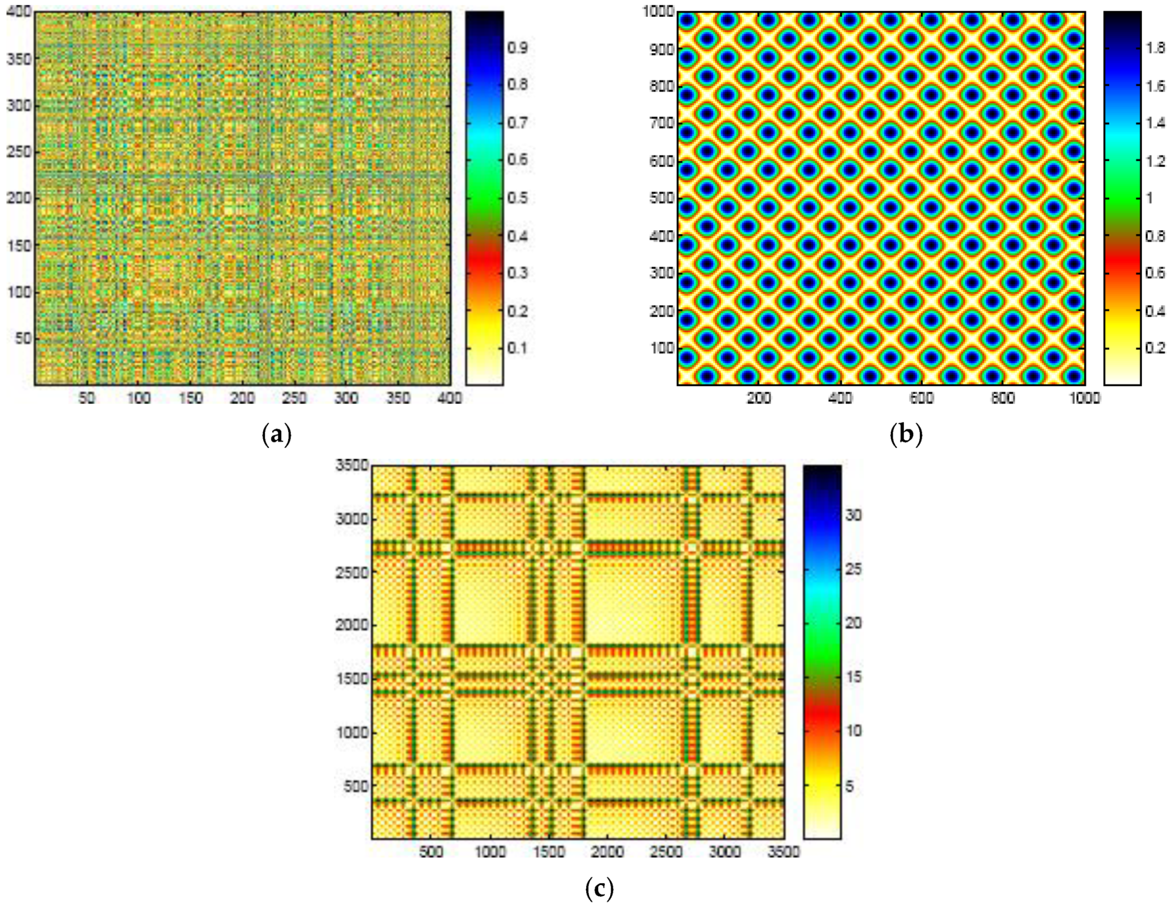
The purpose of RP is to visualize trajectories in the phase space, which is especially advantageous in the case of high-dimensional systems. They are also useful for finding hidden correlations in highly complicated data. Moreover, because they make no demands on the stationarity of a data set, RPs are particularly useful in the analysis of systems whose dynamics may be changing or in high-dimensional systems. Typical patterns are linked to a specific behavior of the system. Therefore, we can distinguish a set of qualitative characteristics that provide two topological approaches: large-scale topologies and small-scale textures.
The large-scale topologies can be classified in homogeneous, periodic, drift and disrupted.
- Homogeneous RPs are typical for stationary systems, as can be seen in Figure 1a.
- Check board-lookalike RPs are periodic and quasi periodic systems, as illustrated in Figure 1b.
- Drift is caused by parameters with slowly varying parameters, and so the RP slowly pales from the LOI (Line of Identity). If the paling is uniformly progressive, this may reflect non-stationarity in the form of a gradual trend.
- Disruptions are caused by abrupt changes in the dynamics.
Figure 1.
Topological characteristics of the recurrence graph: (a) uniformly distributed white noise; (b) a sinusoidal signal; (c) the Lorenz system.
Figure 1.
Topological characteristics of the recurrence graph: (a) uniformly distributed white noise; (b) a sinusoidal signal; (c) the Lorenz system.

The small-scale textures can be: single, isolated points; diagonal lines, parallel with the LOI; diagonal lines, perpendicular with the LOI; vertical and horizontal lines; clusters (Figure 1c).
RPs are largely influenced by reconstruction parameters. Therefore, the value of the reconstruction dimension m must be carefully chosen to avoid the occurrence of both false recurrences and false correlations. The purpose is not to determine exactly how many dimensions the system has, but to use an adequate dimension so that the dynamics of the system can be observed without distortion. According to Takens, the topological structure of the original trajectory is guaranteed if m ≥ 2d + 1, where d is the size of the attractor [13].
Although the importance of the delay in analysis using RP was acknowledged, its influence was little debated. When the delay is too long (irrelevant), diagonal lines appear perpendicularly to the LOI whose length is proportional to the delay. Although this phenomenon can be interpreted when using too small of a dimension, increasing it does not always lead to better results.
A crucial parameter of RP is the threshold ε. Several methods for choosing the threshold are described in the literature, the most common being ε = 10% of the average size of the attractor. However, in general, its size depends on the studied system. In any case, one should keep in mind that if ε is too small, no recurrence point may be identified and no pattern in RP can be determined. If ε is too wide, almost anything will be a neighbor to any other point. Additionally, too high of an ε can include in the vicinity points that are just simple consecutive points on the trajectory. Therefore, a compromise must be made when choosing the value of the threshold ε. In addition, the presence of noise can impose restrictions on the choice of the threshold because noise will distort any existing structure in the RP. By increasing ε, these structures can be preserved [25].
False neighbors can appear in the vicinity of a point on the path in the state space of consecutive points on the same path. These points correspond to the same orbit as the reference point and not to a parallel orbit. This effect is called tangential motion [31] or Thieler autocorrelation and leads to thicker and longer diagonals in RP than they should be in reality.
One of the methods for removing the structures introduced by the tangential motion in RP was proposed by Gao in [32,33], and it is based on considering the difference between the true recurrences and those introduced by the tangential motion.
It is obvious that the number of false recurrence points depends on the choice of neighborhood size, sampling frequency, delay time and reconstruction size. The higher the sampling frequency, the higher the probability of false recurrences occurring in the vicinity.
To eliminate false recurrences, the points belonging to the orbit of the reference point will be identified and removed. The algorithm will continue for all points on the path so that the recurrence matrix from which the false recurrences were removed will be the True Recurrence Matrix (TRM), and its graphical representation is called the True Recurrence Plot (TrRP).
In this article, we outline the nonlinear analysis methods of chaotic dynamic signals. One area of application for the analysis methods using nonlinear time series is that of controlling chaotic dynamical systems by identifying unstable periodic orbits in chaotic time series. Additionally, as a solution, we present a method of two-dimensional representation specific, from the graphical point of view, to the recurrence diagram [34]. A solution to the established problems generated by the classical control methods is represented through the analysis of the nonlinear time series.
3. Control Methods
The theory of dynamic systems deals with the evolution of a system, that is, with the change in its state over time.
A deterministic dynamic system is entirely characterized by its initial phase and its dynamic nature [35]. Such a system can have a continuous or a discrete phase space and a dynamic defined in direct/continuous or discrete time.
A dynamic system in direct time is modeled by a system of differential equations, and the evolution of a dynamic system in discrete time is defined by a system of equations with finite differences [36,37].
The methods of chaos control can be divided into feedback and non-feedback methods. Non-feedback methods use perturbations independently of the stage of the system (control in open loop), while feedback methods use perturbations on the basis of knowing the stage of the system (control in closed loop). Methods can be differentiated also by the type of perturbations, i.e., whether they are in continuous time or discrete [38,39].
The simplest way of curtailing chaotic oscillations is to change the parameters of the system in such a way as to determine the desired type of behavior. Using the bifurcation diagram, we can choose the necessary values of the system parameters for any predefined type of behavior: fixed points, or orbits with one, two or more periods.
This method, known as the resonant parametric perturbation method, is based on the analysis of the bifurcations of the system that needs to be controlled as a function of the control parameters.
Chaos regulation refers to the chaos control through independent phase perturbations or through noise.
The problem of control, in the case of ideal systems in which there is no noise, is reduced to small disturbances to stabilize the chaotic systems of the UPO, which cease after reaching the desired state.
3.1. Identifying the UPO for a Chaotic System
3.1.1. The Adaptive Control of Chaotic Systems
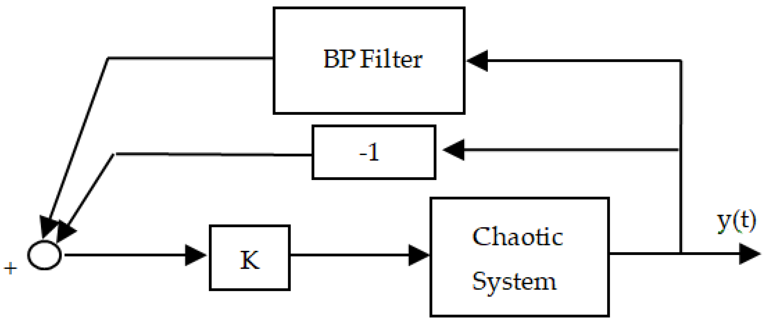
Next, the authors present one of the possible approaches with closed loops to stabilize the unstable periodic orbits [28]. This method relies on perturbing a system variable instead of a control parameter. This feature is preferred in all the cases where the control parameters are strongly influenced by external conditions and their alteration is harder to achieve. To illustrate, we consider the control diagram described in Figure 2.
In the studied adaptive control method, we used a chaotic system characterized by the equations of the Lorentz system, with the output of the system y(t) being described by the state x2 of a system based on differential equations that describe the evolution of the system. As can be seen in Figure 2, the output of the system y(t) is passed through a bandpass filter and, at the same time, is inverted. After summing the two processed signals and amplifying them with a constant K, the resulting disturbing signal is described by the following equation,
Following the previous processing, a sinusoidal signal results at the output of the adaptive control system [40,41].
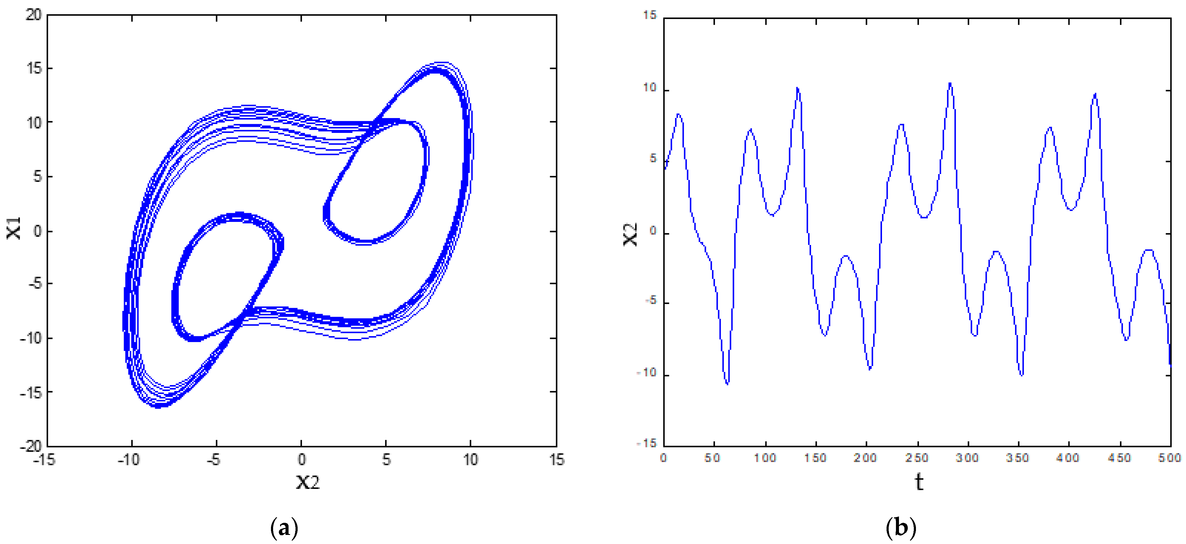
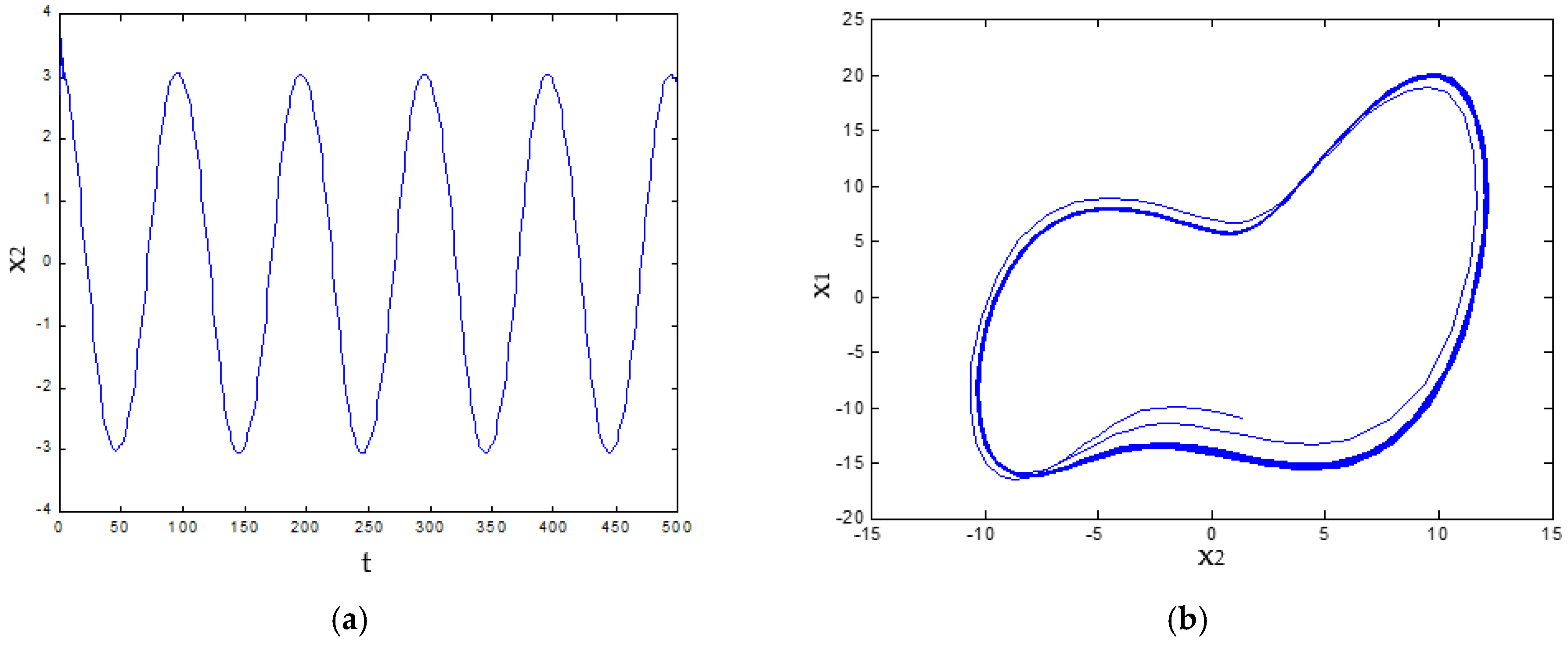
The evolution of the Lorentz system, described by the state x2 of the differential equation system (t, x2), is shown in Figure 3b, and the chaotic attractor (x2, x1) is shown in Figure 3a.
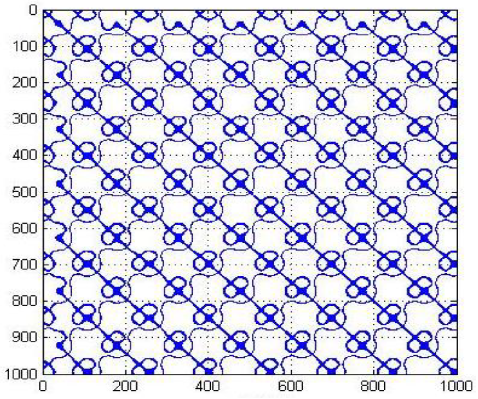
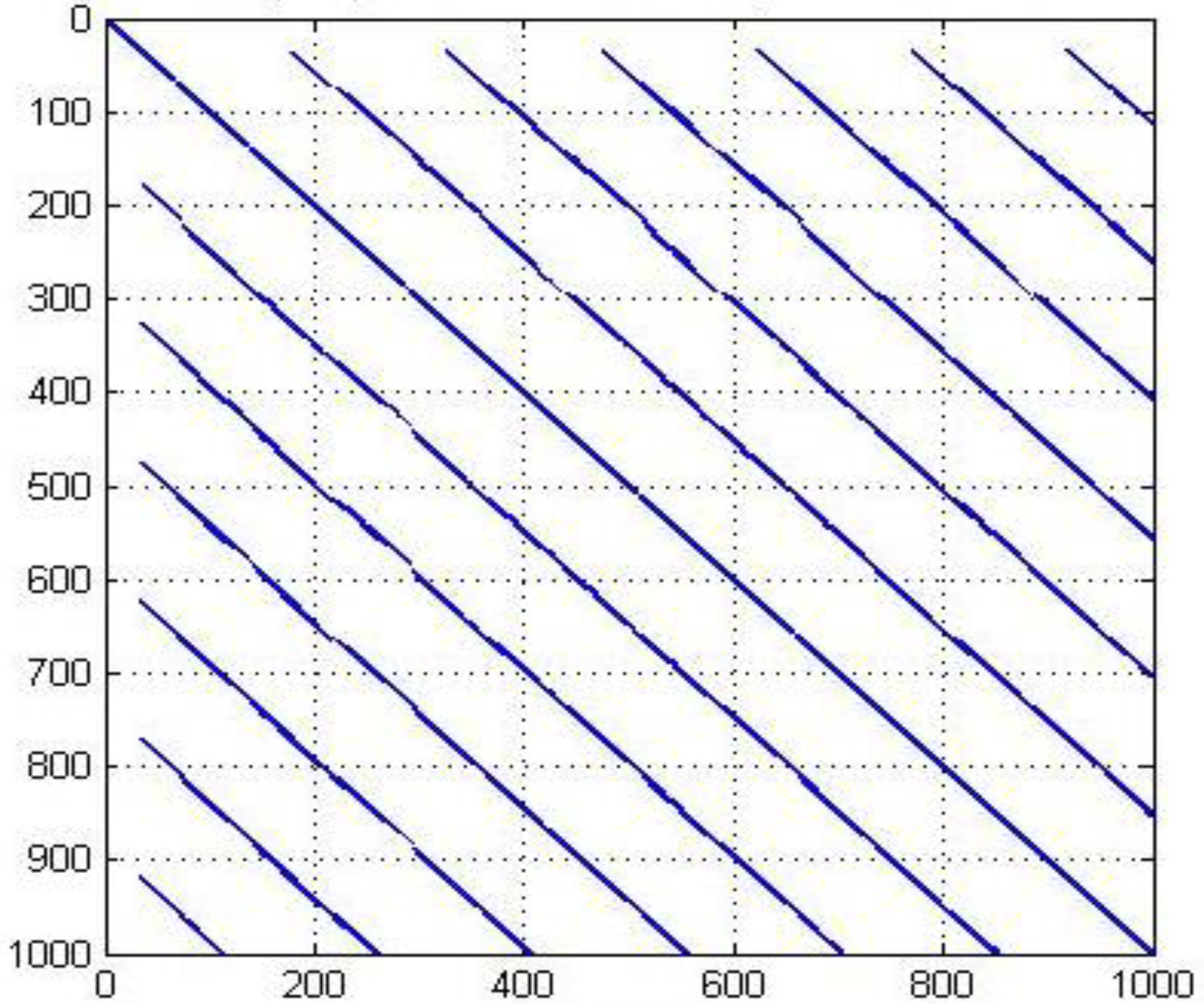
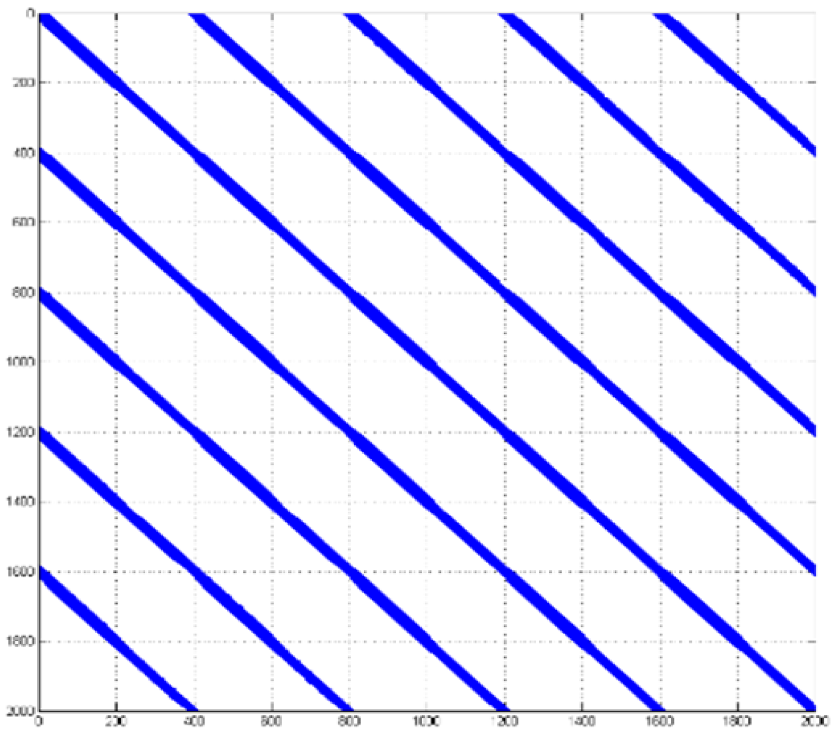
The following figure shows the recurrence plot for the trajectory in the phase space (x2, x1) of the Lorentz system. The representation algorithm consists of allocating a blue dot for each point in the two-dimensional graph if the distance is less than a set threshold value, and white for the rest.
The identification of unstable periodic orbits through a more precise method was the purpose for which the concept of recurrence plots applicable to chaotic time series were introduced [29,42]. The principle of UPO identification is that when the trajectory of the chaotic system is near an UPO, the trajectory will remain in the vicinity of the UPO for a period of time that depends on its instability.
Correspondence in the recurrence plot of the principle, described above through shapes in accordance with the periodic movements, is an uninterrupted distribution, equally, of diagonal lines. Additionally, additional information that we obtain relatively easily about the moment and the time interval when the chaotic system has close behaviors are provided in the recurrence plot by the position of the lines and their length. Thus, information regarding the state of the chaotic system at a given time is provided in the recurrence plot by the short lines and the isolated points tell us that it will not return to that state. In contrast, if the system tends to a stable state, it will have a corresponding long line in the recurrence plot. The information in the recurrence plot regarding the length of the lines and their position is the necessary data for the identification of the periodic behaviors. In other words, by selecting lines larger than a specified value, parallel to the LOI, the UPO is identified from the evolution of the system.
In Figure 4, we can easily notice periodic forms. This observation can lead us to the idea of using a recurrence plot for identifying unstable periodic orbits in chaotic time series.
In Figure 3a, we can notice parallel evolutions of the orbits in the phase space, which, in the recurrence plot in Figure 4, form lines of different lengths parallel to the main diagonal.
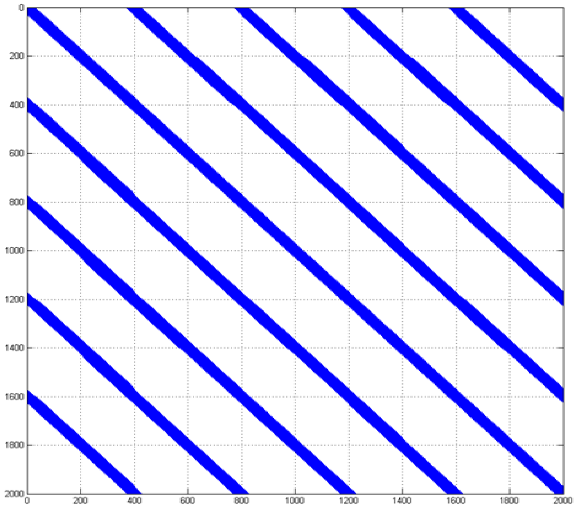
If in the recurrence plot in Figure 4 we apply a filtration using a high threshold, we obtain the Figure 5.
The recurrence plot representation in Figure 5 for the filtered chaotic signal corresponds to a quasi-sinusoidal signal obtained from the Lorentz chaotic system by using the control method described in Figure 2.
To determines the parameters of the control system so that the recurrence plot for the filtered chaotic signal is made to correspond to a recurrence plot for the controlled signal, we used an optimization algorithm based on evolutive strategies.
3.1.2. The Optimization of the Adaptive Control Algorithm Using Evolutionary Strategies
For the optimization of the coefficients of the adaptive control through evolutive strategies (ES), we chose the principle (2 + 2), where there are two parents with two descendants after evaluating the first generation.
In adaptive control, obtaining the evaluation function for the individuals in a generation involves stabilizing the system on an unstable periodic orbit by using a perturbing signal by minimizing the amplitude variations of the controlled signal.
where and x is a sinusoidal entrance signal with various amplitudes.
Thus, we have the initial solution , for which and are calculated.
We evaluate (for the initial solution):
- We modify
![Electronics 11 00947 i001]()
- We evaluate ;
- If , then the new population will be ; however, if , then the new population stays .

We repeat steps 1, 2 and 3 until we obtain the desired result. We have to mention that this optimization process does not involve finding the ideal solution.
For implementing adaptive control, we have to consider an example with a concrete calculation.
The values of the coefficient where we start the optimization are and . Within this optimization process, the error evaluation function was achieved to obtain a signal with a constant amplitude. The values of the coefficients after optimization are and .
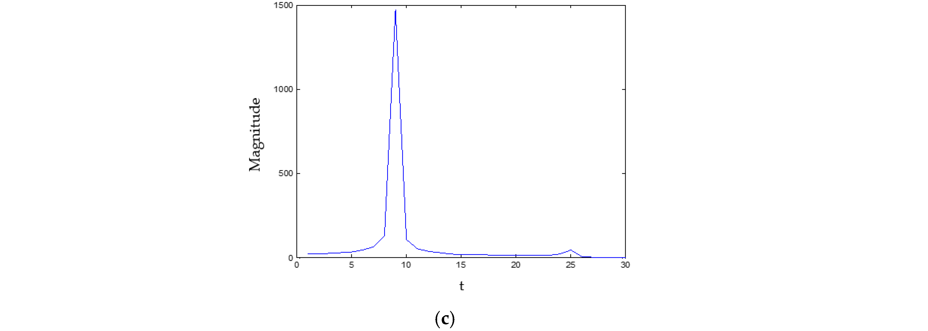
The resulting quasi-sinusoidal signal and its representation in the phase space are shown in Figure 6a,b. Figure 6c shows the Fourier transformation of the quasi-sinusoidal signal obtained from the chaotic system. We notice that the signal specter is focused on the 7.8 Hz frequency, which is the crossing frequency of the filter cross band from the control diagram in Figure 2.
Some of the control methods (non-feedback methods) exploit certain properties of the system or information about the system and modify it by changing a control parameter so that the system moves from a chaotic attractor to a periodic phase. This method, known as the method of parameter variation, relies on the analysis of the bifurcations of the system that needs to be controlled as a function of the control parameters.
The paper covers another method for the analysis of chaotic systems, the recurrence plot method (RP), with the help of which we can identify the periodic stages in a time series. This time series is the output of the chaotic system.
Therefore, we obtained a method of analysis for adaptive control systems, by using RP, which helps to identify the periodic stages in chaotic systems by keeping from the RP only those lines parallel to the main diagonal and whose length is greater than a certain threshold value.
We proposed a method for optimizing the performance of control methods for chaotic systems that is optimization through evolutive strategies relating to adaptive control, which leads to the discovery of the coefficients that are part of the control methods.
3.2. Chaos Control in the Buck Converter
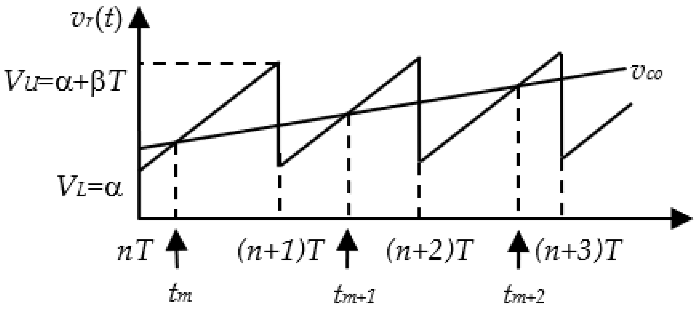
The analyzed buck converter is a low-voltage converter, direct current–direct current, with a width modulation of control pulses characterized, depending on the values of the circuit parameters, by a diversity of behaviors [43].
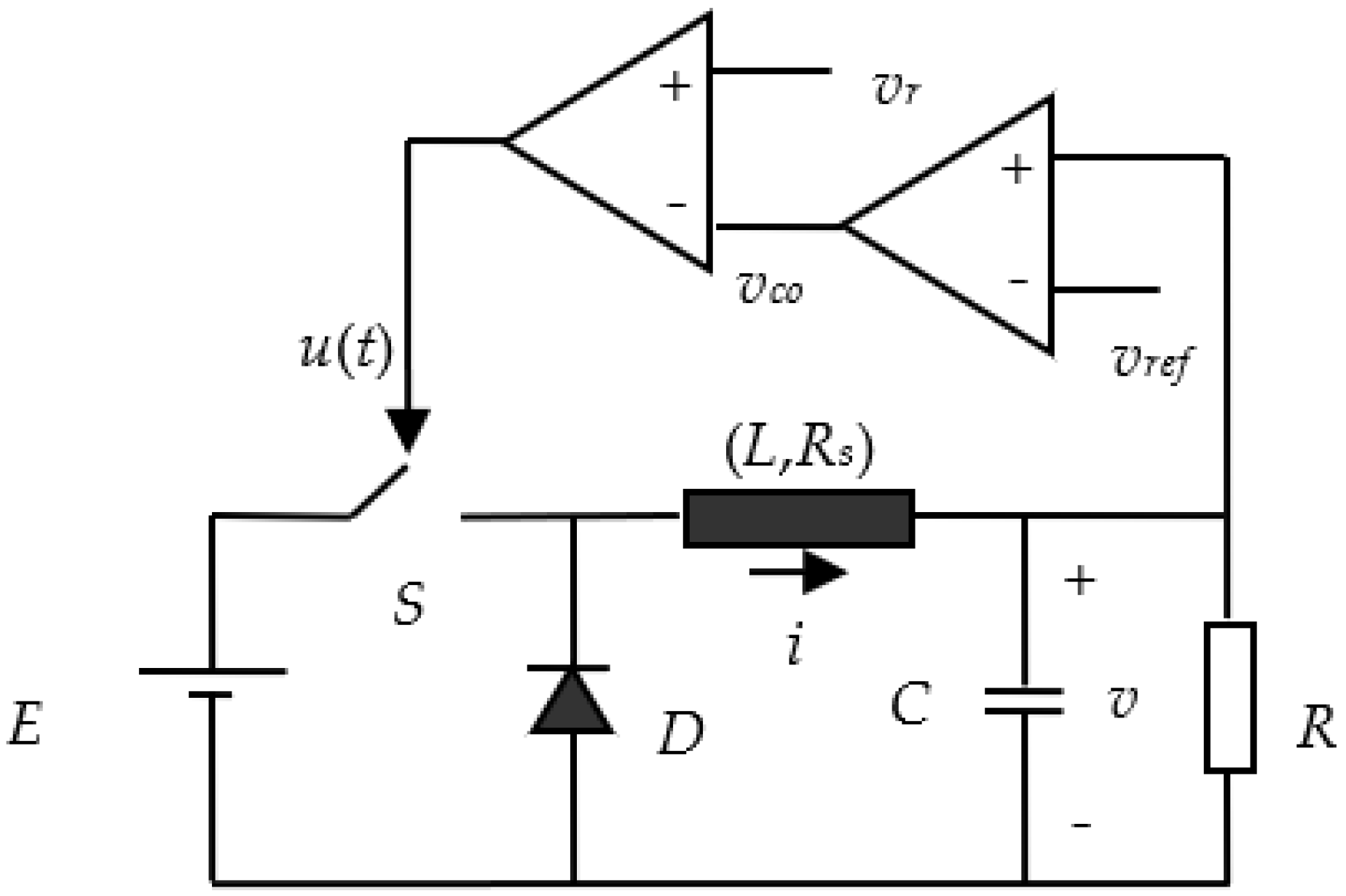
Next, the evolution in the state space of the buck converter (Figure 7), controlled in PWM (Pulse Width Modulation) voltage, is studied with its operation in continuous conduction mode.
The operation of the converter is characterized by the following system of differential equations:
where E is the supply voltage, i is the current through the coil, v is the voltage across the capacitor and u(t) is the Pulse Width Modulation (PWM) control signal, which for closes the switch S and for open switch S [44,45,46].
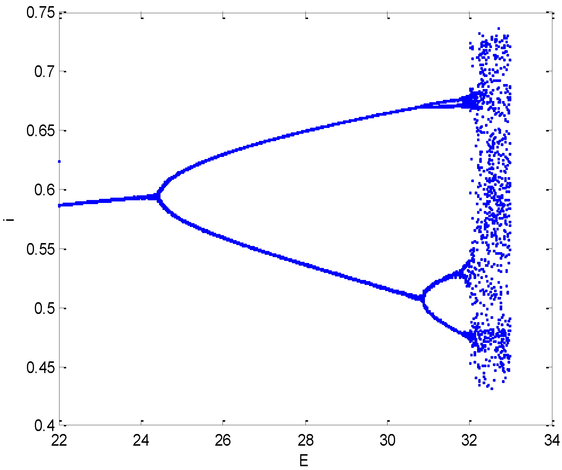
A way to visualize the dynamic behavior of the buck converter (the parameters of the buck converter are given in Appendix A) is the bifurcation diagram, exemplified in Figure 9, where the evolution towards chaos is achieved by changing the supply voltage between 22 and 33 V.
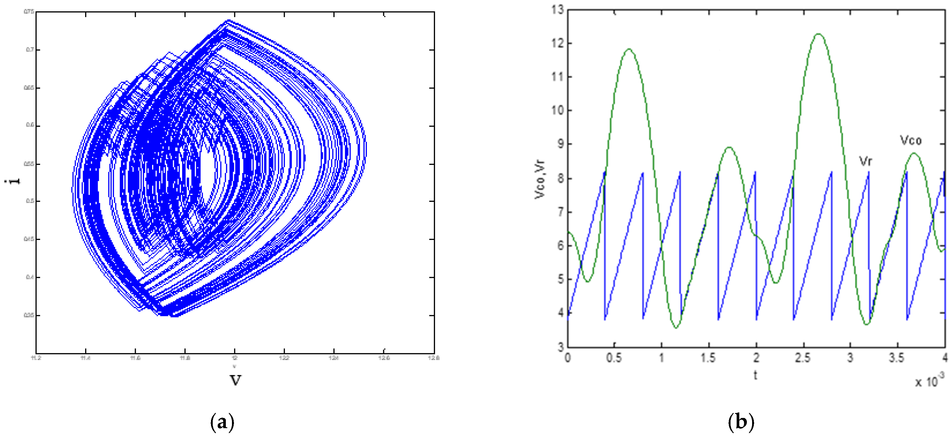
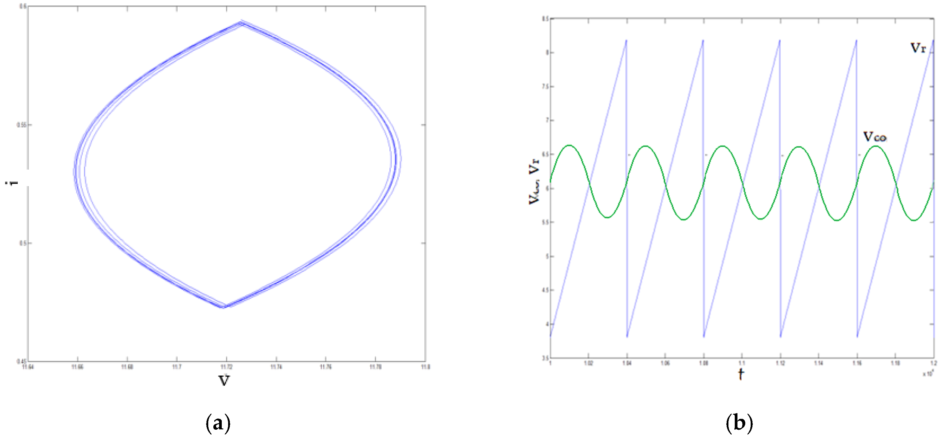
According to the previous graph, the buck converter exhibits chaotic behavior for supply voltage values over 32.27 V. Figure 10a,b illustrate, for a supply voltage of 33 V, the evolution in the state space and the control voltages of the buck converter.
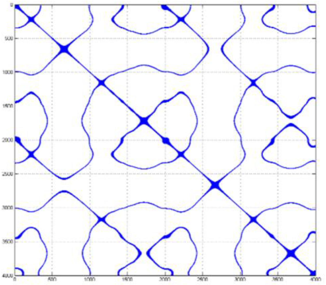
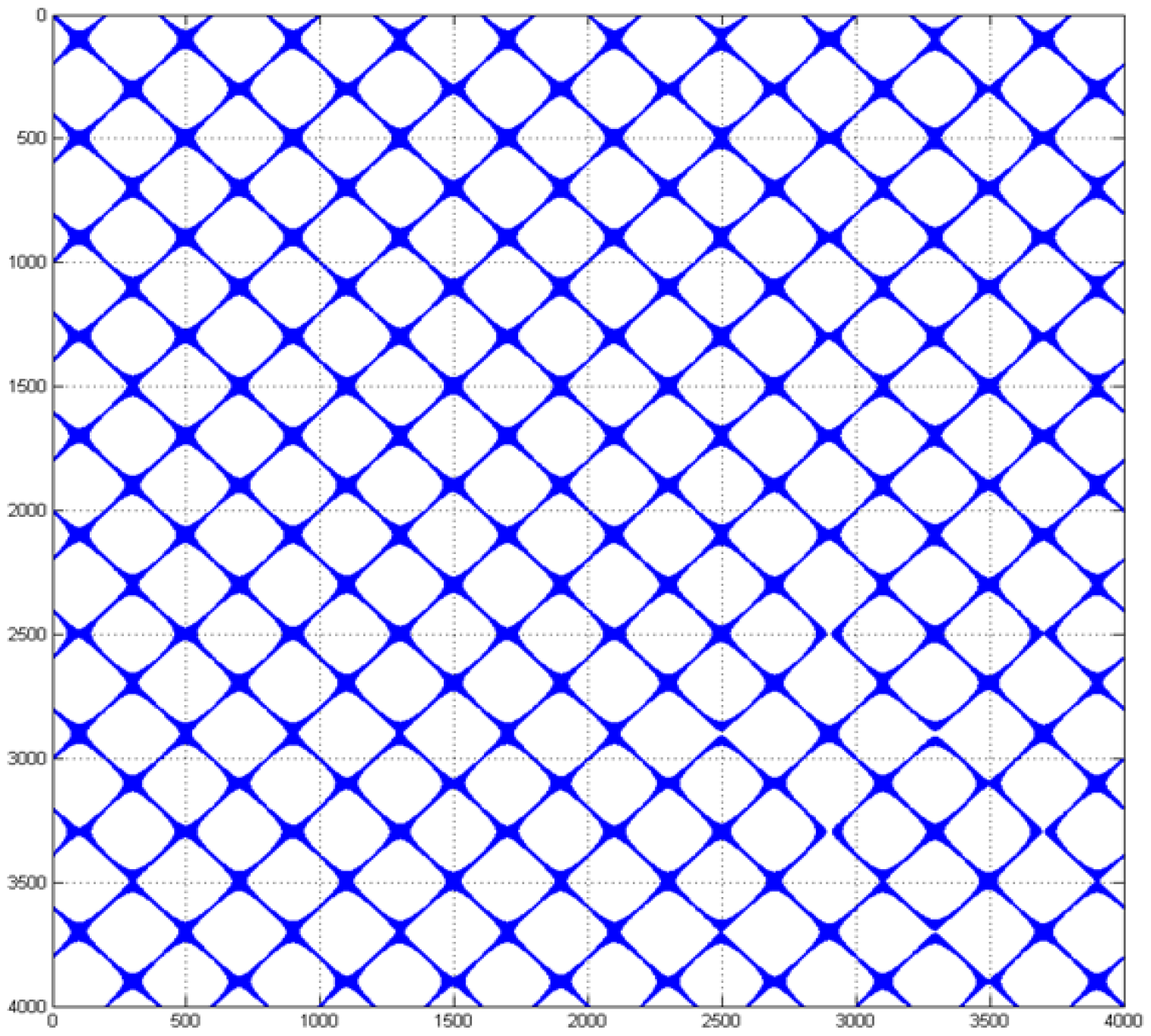
By applying the recurrence plot to the output signal for a chaotic regime of the buck converter at a supply voltage of 33 V, the plot in Figure 11 is obtained.
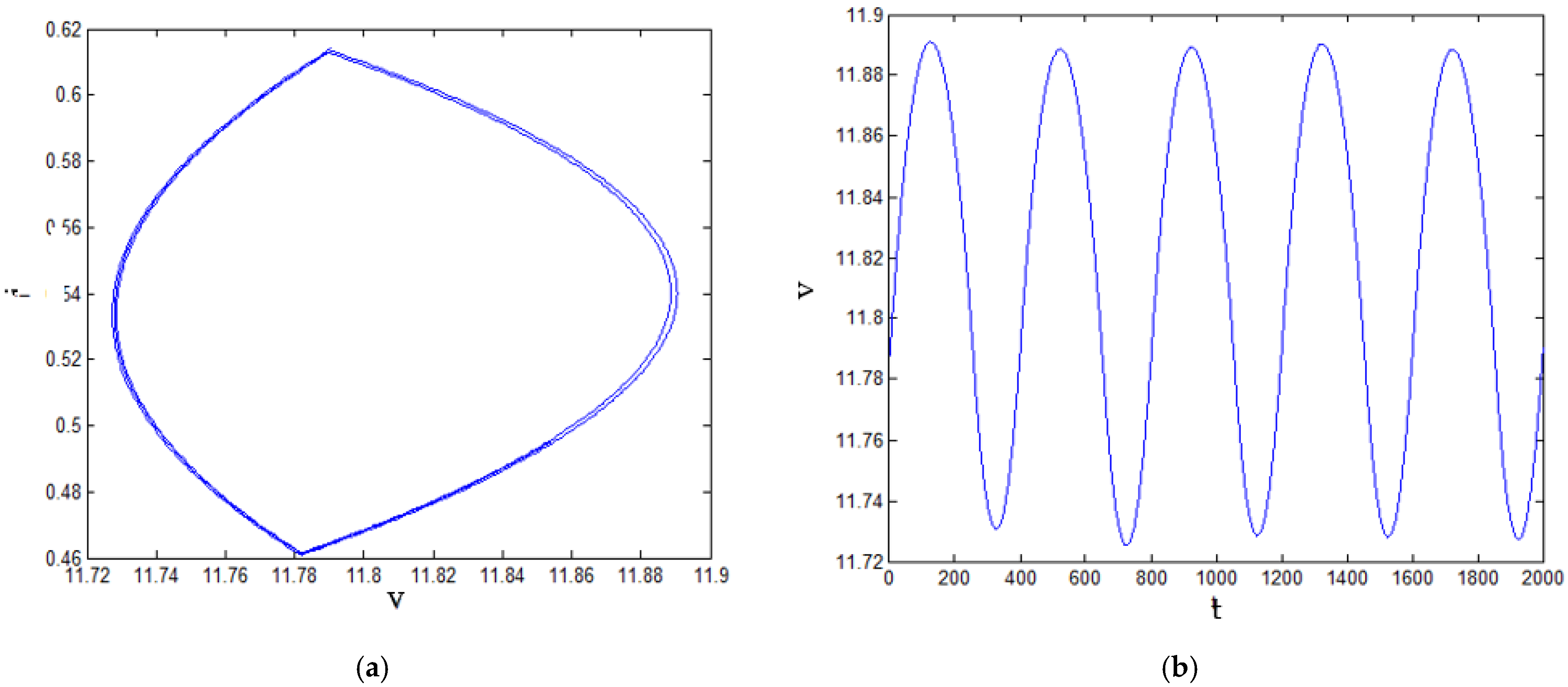
Until it reaches its chaotic state, the system crossed periodic states, of various lengths, corresponding to a certain charging voltage. Thus, for a charging voltage E = 24 V, the converter exhibits a periodic behavior from period one, as shown in Figure 12.
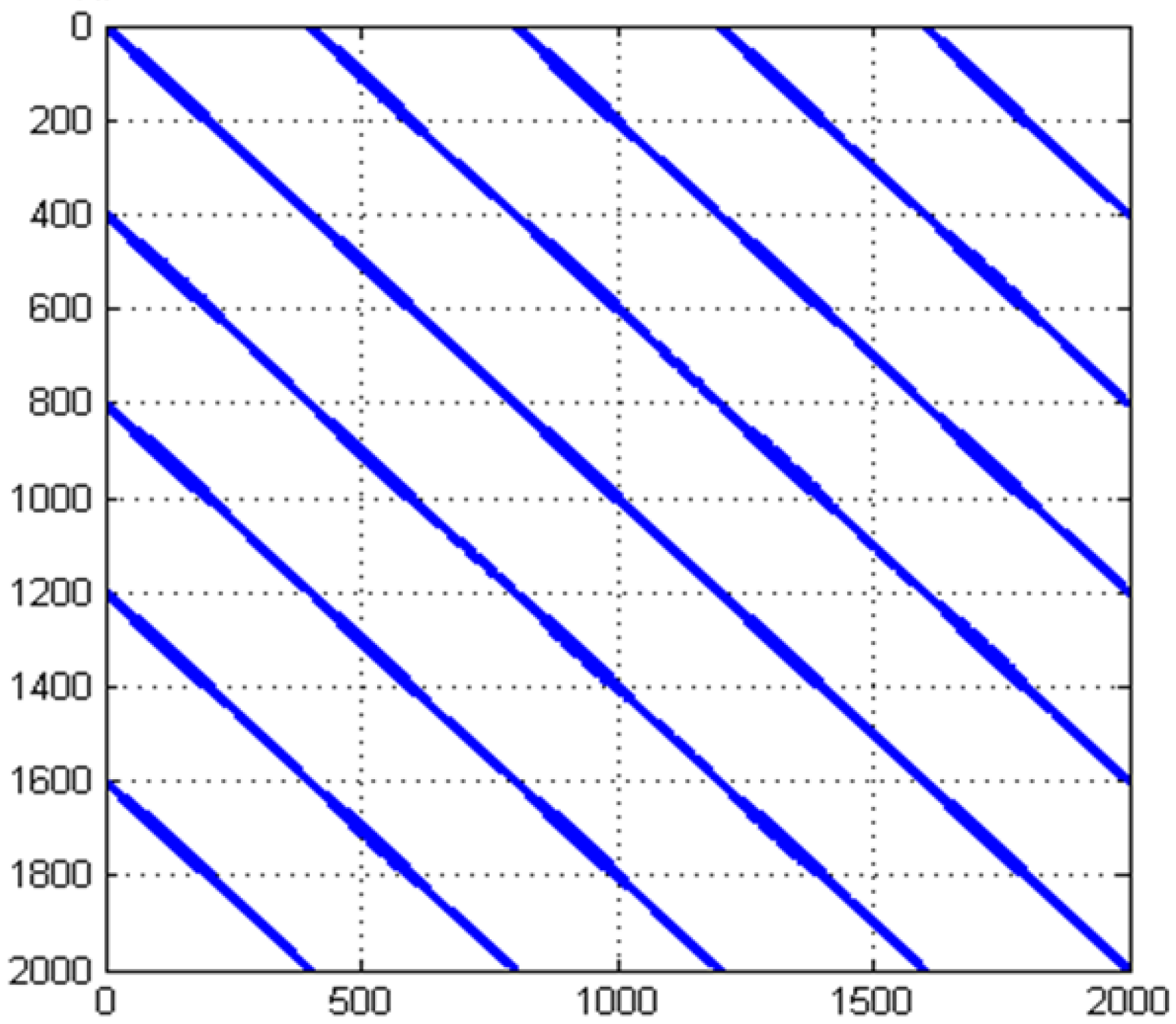
By applying the recurrence plot to the output signal for a periodic regime of the buck converter at a supply voltage of 24 V, the plot in Figure 13 is obtained.
3.2.1. Control of the Buck Converter via the Method of Disturbing Parameters
The control of the buck converter that works in chaotic mode, for a supply voltage of 33 V, is achieved via the method of disturbing the parameters. To exemplify this method, the disturbed parameter was applied as follows,
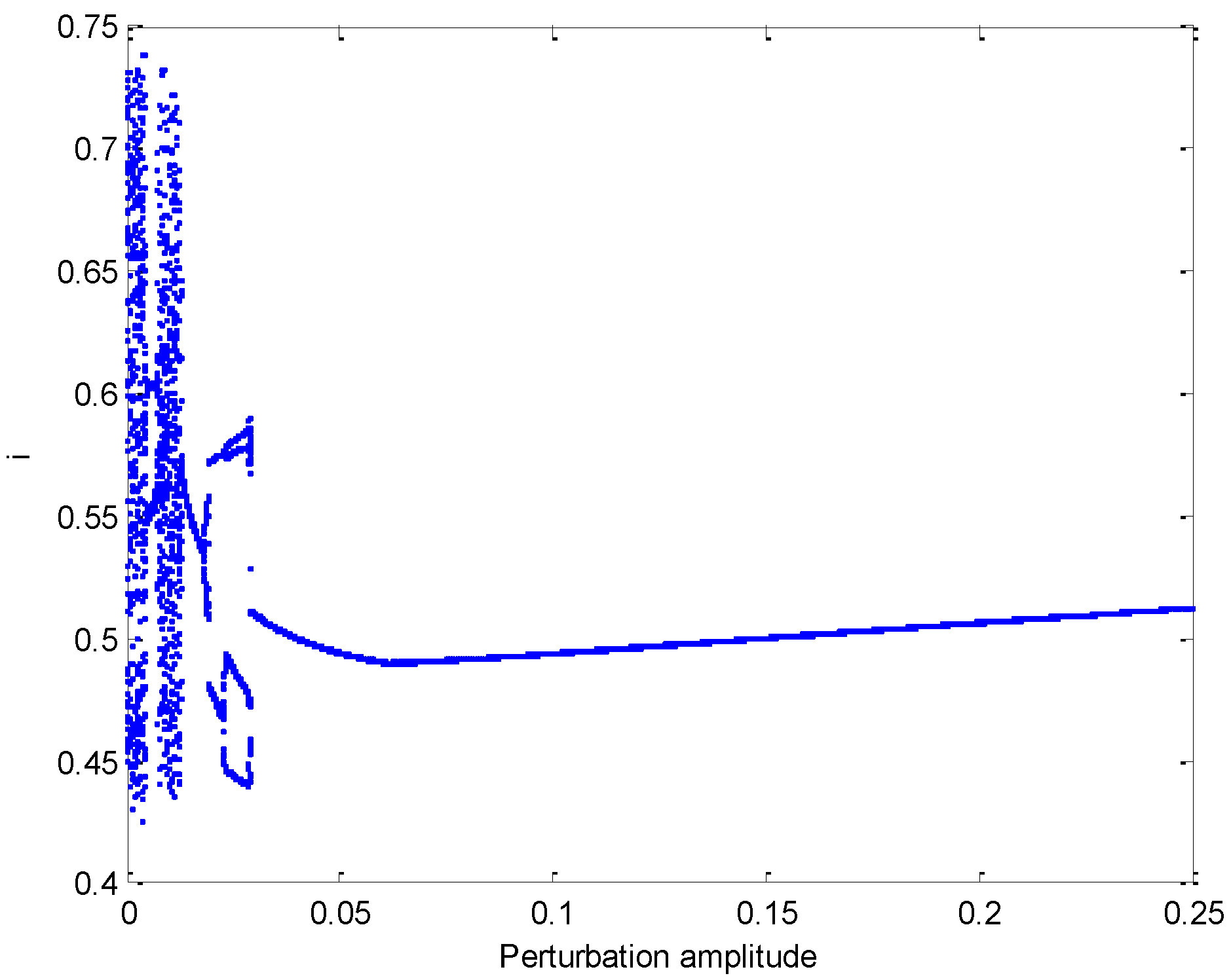
noting the amplitude of the control signal with α and the frequency of the control signal with f. Next, to exemplify the efficiency of the control method, the amplitude of the disturbing signal is modified in the range 0 ÷ 0.25, thus leading to a study on the dynamics of state terms by drawing in Figure 14 the bifurcation diagram, a graphical representation of the induction current i versus the amplitude of the control signal α.
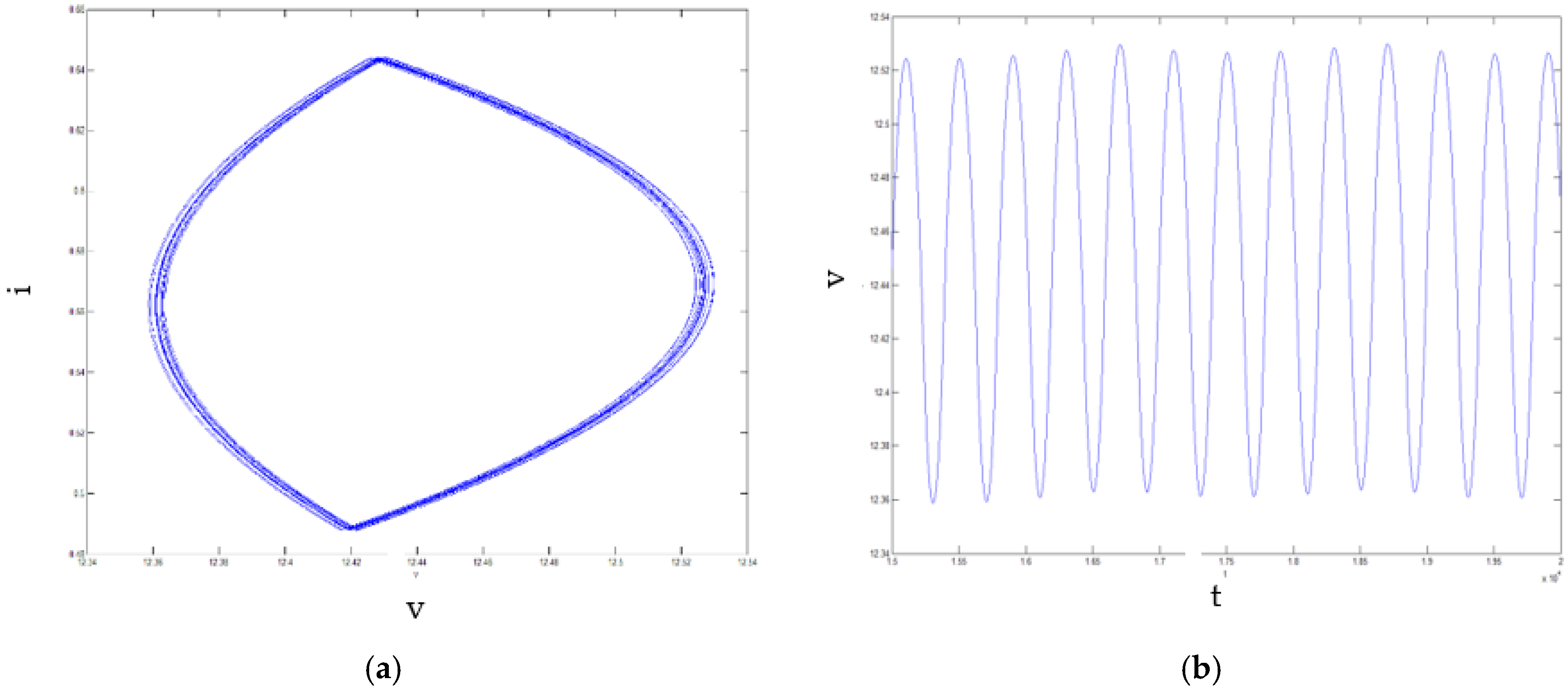
Analyzing the previous bifurcation diagram reveals the efficiency of the buck converter control method when applying the disturbing signal. Figure 15a illustrates the chaotic attractor of the buck converter controlled by the method shown above for a disruptive signal amplitude of 0.2. The output signal of the buck converter controlled by a disturbing signal is illustrated in Figure 15b.
By applying the recurrence plot to the output signal of the controlled buck converter at a supply voltage of 33 V, the plot in Figure 16 is obtained.
When studying the behavior of the buck converter by analyzing the recurrence graphs, it is observed that the RP related to the output signal of the system controlled by the parameter disturbance method, at a supply voltage of 33 V, shown in Figure 16, is similar to the RP related to the output signal for a periodic regime of the system at a supply voltage of 24 V.
In other words, the RP of a UPO, the component of the evolution in the state space of the output signal of the buck converter controlled by the method of disturbing the parameters, at a supply voltage of 33 V, shown in Figure 16, is similar to the RP of a UPO for a periodic mode of the converter at a supply voltage of 24 V.
Since the UPO is a component of the evolution in the state space of the output signal of the buck converter, at a supply voltage of 33 V, i.e., in an RP related to the chaotic behavior of the buck converter, we recognize the lines parallel with the LOI corresponding to the periodic behavior of period one.
In other words, the authors found that the RP related to the output signal of the system at a supply voltage of 33 V, for which only the lines parallel with the LOI greater than a specified value are kept, similar to the behavior for a supply voltage of 24 V, is the same as the RP representation in Figure 16.
The recurrence plot of the unfiltered output signal of the buck converter for E = 24 V is shown in Figure 13 and the recurrence plot for the filtered output signal is given in Figure 17.
Under these conditions, when analyzing the behavior of the buck converter controlled by the method of disturbing the parameters, we see that, at small amplitudes of the control signal (the lowest effective value of the amplitude of the disturbing signal), the stabilization is not satisfactory.
3.2.2. Control of the Buck Converter with a Phase Difference Signal
Furthermore, for the optimization of the previous control method applied to the buck converter, a control signal with phase difference θ between the disturbing signal and the sawtooth signal is used:
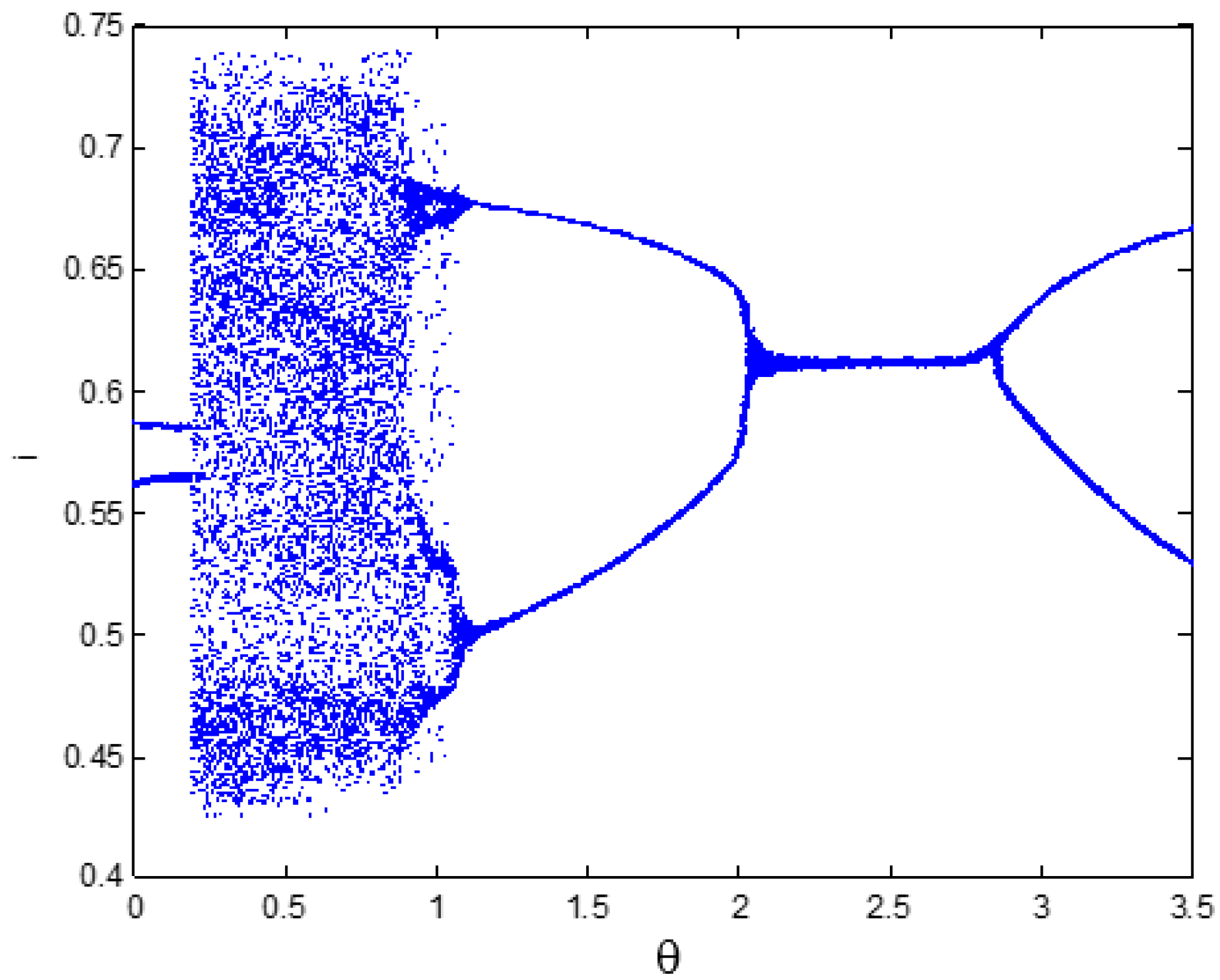
where the switching frequency of the buck converter has been noted with fs. For a clearer description of the previous control relationship, we can say that the sawtooth signal is directed by the disruptive signal with a phase shift θ. Next, to visualize the behavior of the buck converter controlled with a phase difference signal, with an amplitude value much lower than the lowest effective value of the disturbance signal amplitude, the bifurcation diagram is used that has the phase shift as a bifurcation parameter.
The graphical representation from Figure 18 is made for a value of the amplitude of the disturbing signal of 0.0035. Analyzing the behavior of the controlled buck converter according to the previous bifurcation diagram, it is observed that the system can be stabilized on the stable region of period one for α = 0.0035, at a phase difference of between 2 and 2.6. It can also be stated that for α = 0.0035, the stable region of period one is equidistant from θ = 2.3 and, thus, the chosen phase shift is an optimal phase difference for this particular case.
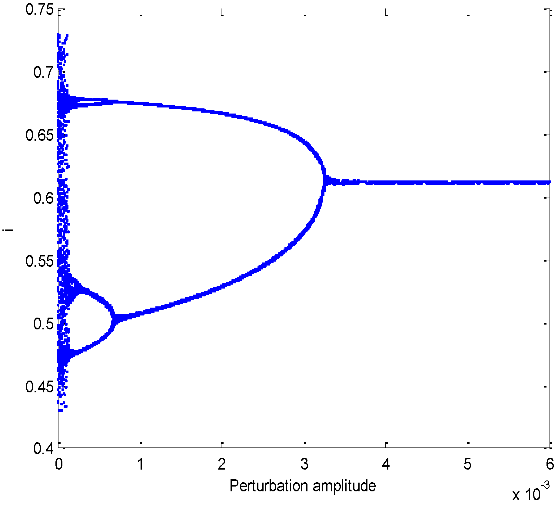
Further, when examining the optimal phase difference by plotting the bifurcation diagram of the controlled buck converter i(α) (Figure 19), it is observed that the system can be stabilized in the stable region of period one for a 0.0034 minimum value of the disturbance amplitude, a value much less than the in case of not using a control signal with a phase difference.
In these conditions, according to the bifurcation diagram of the buck converter, we still use, for the stabilization of the stable region of period one, a control signal with the amplitude of the disturbance α = 0.0035 and the phase difference θ = 2.3. The chaotic attractor of the buck converter controlled by a phase difference control signal θ between the disturbing signal and the sawtooth signal is illustrated in Figure 20a. The output signal of the buck converter controlled by a disturbing signal with a phase difference is illustrated in Figure 20b.
By applying the recurrence graph of the output signal of the buck converter controlled by a disturbing signal with a phase difference, at a supply voltage of 33 V, the graph in Figure 21 is obtained.
When studying the behavior of the buck converter by analyzing the recurrence graphs, it is observed that the RP related to a UPO, a component of the evolution in the state space of the output signal of the buck converter controlled by a perturbed signal with a phase difference, at a supply voltage of 33 V, shown in Figure 21, is similar to the RP of a UPO for a periodic regime of the converter at a supply voltage of 24 V.
In other words, the authors found that the RP related to the output signal of the controlled system at a supply voltage of 33 V, for which only the lines parallel to the LOI higher than a specified value are kept, similar to the behavior for a supply voltage of 24 V, is the same as the RP represented in Figure 17.
3.2.3. Control of a DC Motor Using the Buck Converter
The final application showing the advantages of using these analysis methods in the control of dynamic systems relates to the control of a DC motor with permanent magnets, using the previously analyzed buck converter, a DC converter, through a filter to reject any disturbances from the inductive effect of the DC motor, a piece of equipment usable in nuclear research.
The issue of controlling the speed is one of the key issues in relation to designing systems with electric command, with the type of command motor depending on the tool and technological process used. Controlling the speed of a system with electric command involves an external intervention in the system’s functional parameters, either with the intent of moving the system from a stable speed to another one or to maintain a constant working speed for the system.
The control of the rotation of the direct current motor is achieved by changing the charging voltage of the motor’s inductor. The buck converter is used to vary the charging voltage at the inductor in 0–Umot, where Umot is the nominal voltage of the motor.
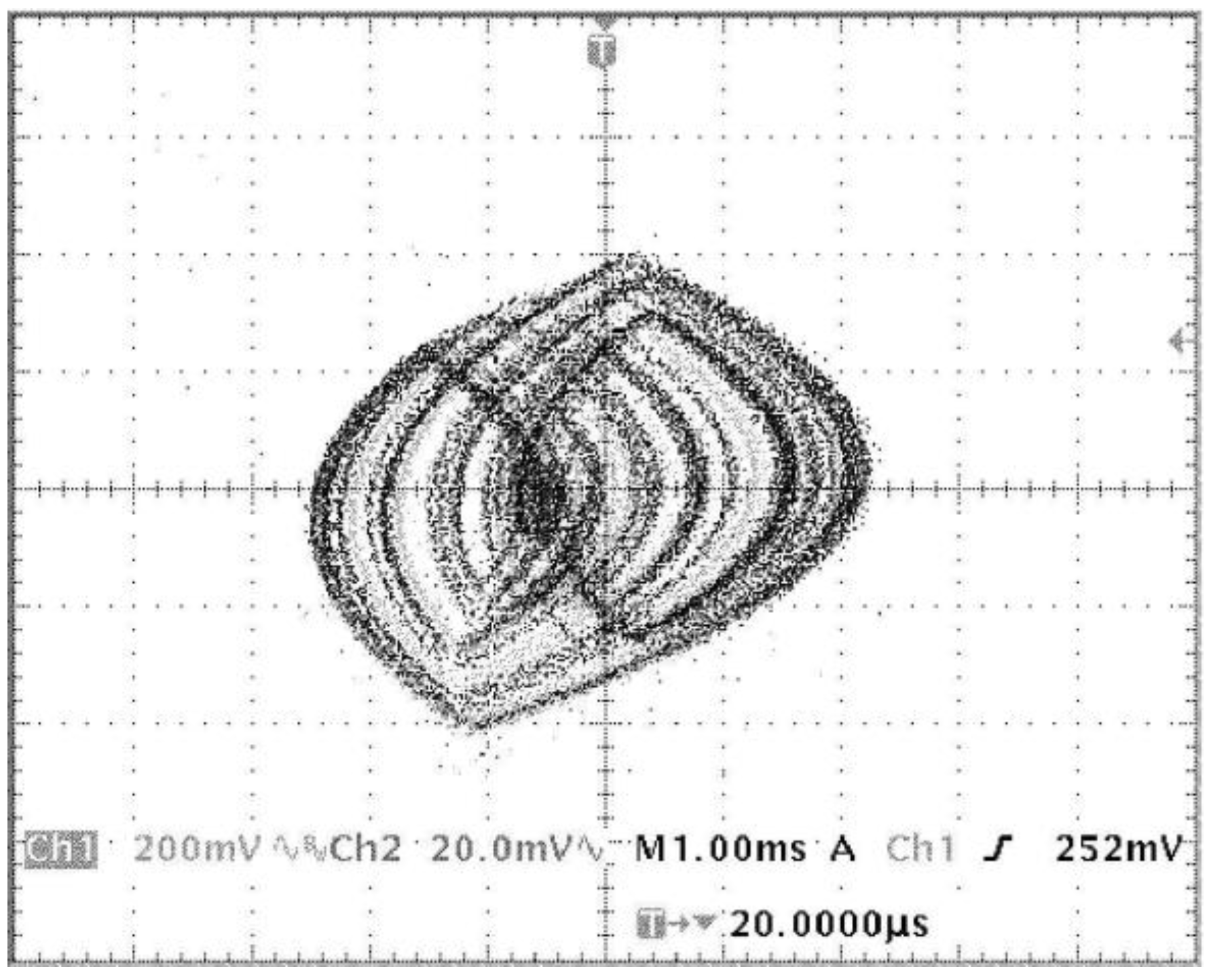
The experimental model was designed to be used for the command of a direct current motor similar to the system we analyzed and simulated previously. Thus, for a charging voltage E = 33 V, the converter exhibits chaotic behavior, as shown through the chaotic attractor in Figure 22.
Because the system exhibits chaotic behavior, we need to stabilize it by applying a perturbing signal to the Vref parameter. The method we chose to stabilize the buck converter at a charging voltage E = 33 V is the method of parameter perturbation.
The trajectory in the phase space of the chaotic system controlled through the parameter perturbation method, with α = 0.2 and a frequency equal to that of the leading signal, is shown in Figure 23a.
The sawtooth signal and the perturbing signal used to control the chaotic system through the parameter perturbation method when α = 0.2 with a frequency equal to the leading signal are shown in Figure 23b.
In this graph, we clearly notice the effect of the stabilization when we apply the perturbing signal. To improve the results at small amplitudes of the perturbing signal, we are using a signal with a phase difference θ between the perturbing signal and the sawtooth signal.
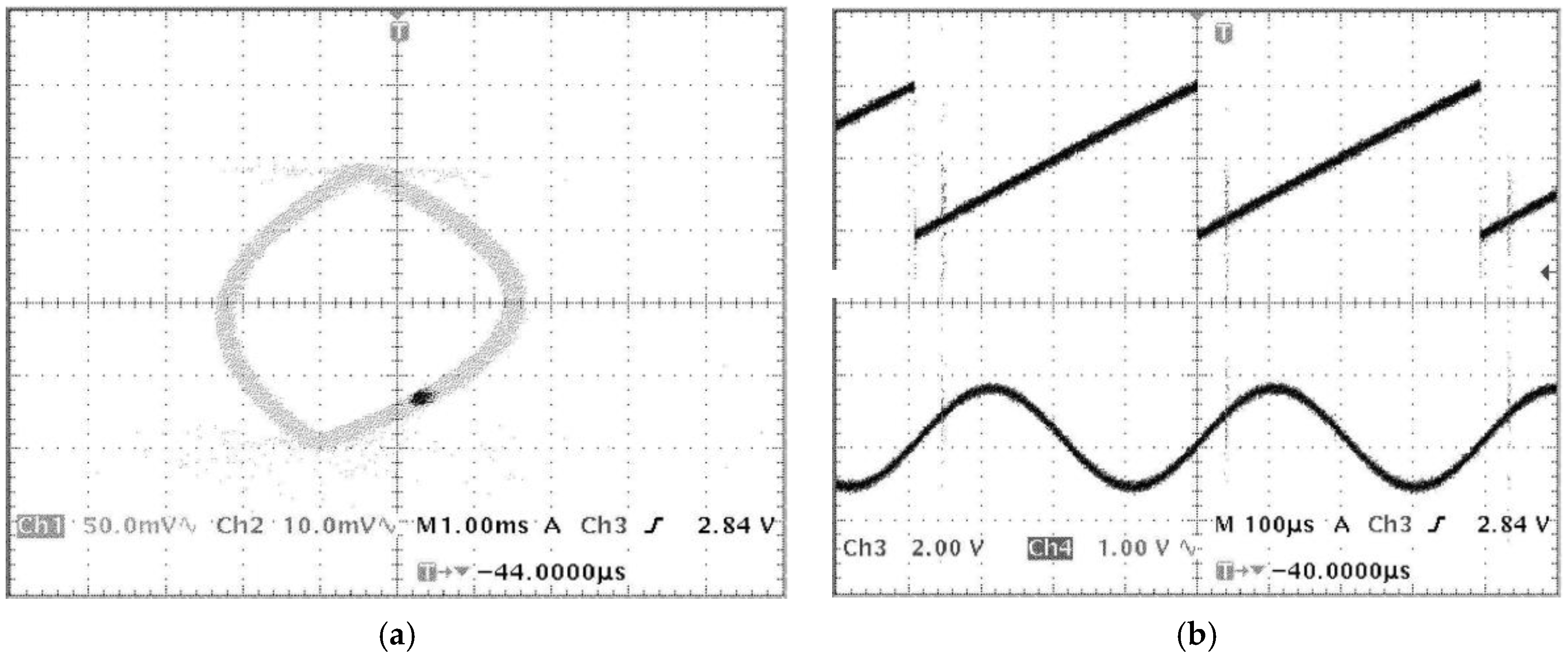
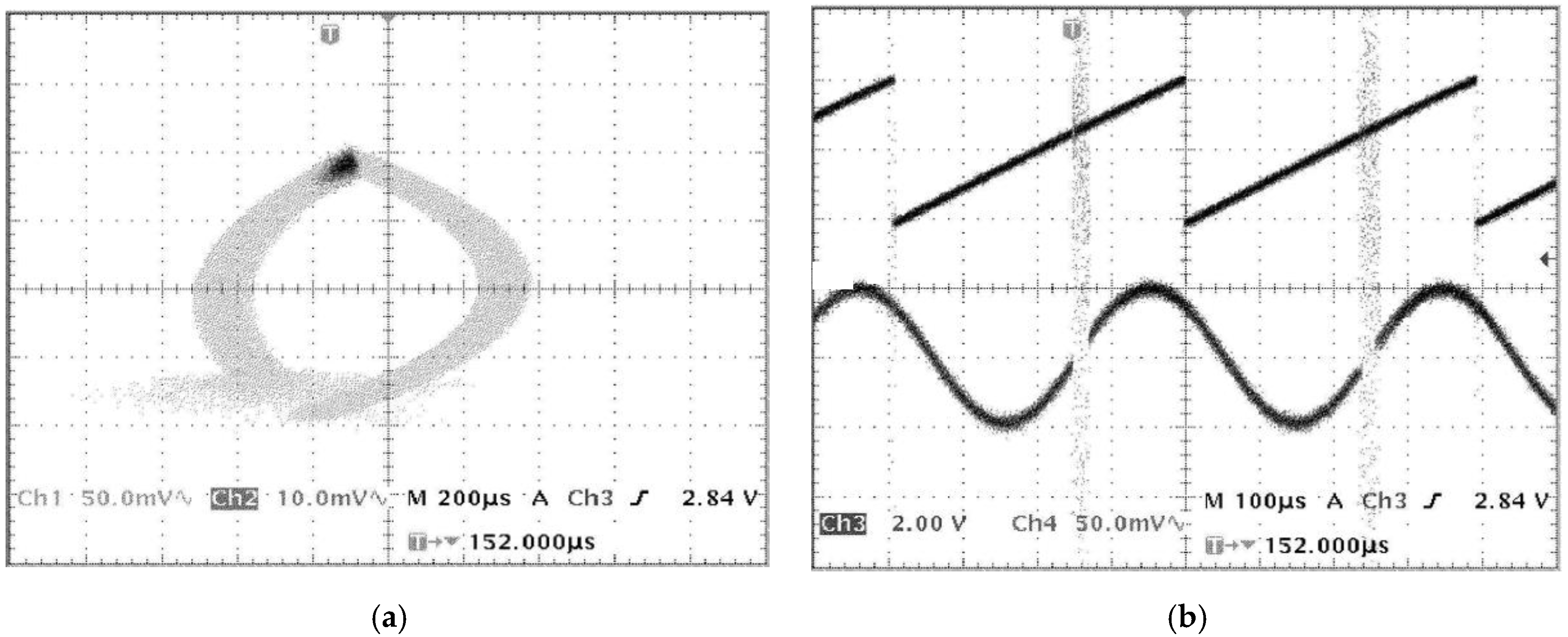
The trajectory in the phase space of the controlled chaotic system when we apply a perturbing signal with the perturbation amplitude α = 0.0044 and a phase offset θ = 2.3, which puts us in the operating area of period one, is shown in Figure 24a.
The sawtooth signal and the perturbing signal used to control the chaotic system with the perturbation amplitude of α = 0.0044 and the phase offset θ = 2.3, which put us in the operating area of period one, are shown in Figure 24b.
4. Results
Through the adaptive control method, we exemplified the possibility of identifying an unstable periodic orbit within a chaotic system. We also used an optimization method with evolutionary strategies to determine the parameters necessary to identify the unstable periodic orbit. As a novelty, we used the recurrence plot to identify the unstable periodic orbit, which is much easier and more accurate than the previous classical method.
Continuing the research, for the control of a system with chaotic behavior (buck converter), we applied the recurrence graph method. Thus, we identified stable behaviors that led to a significant reduction in control power, more easily and more accurately than in the case of classical control methods.
We obtained an analysis method by using RP for buck D.C-D.C. converters, with the help of which we can identify the periodic phases in the chaotic system through the parameter perturbation control method when we apply a perturbing signal with a phase difference.
The designed experimental circuit confirmed the good choice of the control method, which uses a signal with a phase difference θ between the perturbing signal and the sawtooth signal.
As we can see, the initial chaotic system can be stabilized in the operating area of period one by applying a signal with a phase difference θ between the perturbing signal and the sawtooth signal, with an amplitude of the perturbing signal that was much smaller than in the case of the control by using the parameter perturbation method, which uses a frequency equal to that of the leading signal.
The experimental results we achieved confirm the control method needed to stabilize the system regarding charging an engine of direct current with permanent magnets.
Thus, we showed that the strength of the control could be significantly reduced by applying a perturbation with a phase difference between the perturbing signal and the sawtooth signal. Moreover, when we have phase changes in the perturbation, the system exhibits chaotic behavior and can be stabilized by exercising greater control over it [49,50].
5. Discussion and Conclusions
The paper presents a way to solve the problems generated by the classical control methods, for which it was tried for a long time to find a solution, by using nonlinear time series analysis. Among the problems analyzed, we list the identification of stable behaviors (unstable periodic orbits) in chaotic time series and the significant reduction of the control power used.
The initial chaotic system can be stabilized by applying a signal with a phase difference between the perturbing signal and the sawtooth signal with an amplitude of the perturbing signal much smaller than in the case of the control by using the parameter perturbation method, which uses a frequency equal to that of the leading signal. As demonstrated, the control power could be significantly reduced by applying a phase difference signal between the disturbing signal and the sawtooth signal.
Moreover, we proposed a method of identifying the UPO in the time series at the output of the chaotic system.
We can also mention the possibility of using the new methods based on evolutive strategies (ES), aiming to optimize the function of the control methods for implementation in electronic system for achieving good performance from the studies systems.
The authors’ contributions are highlighted by using the RP analysis method in controlling the behavior of dynamic systems and in identifying the type of behavior of the dynamic system.
The study on the command of a direct current motor by using a buck converter shows, through a final concrete application, the advantages of using RP analysis methods in controlling dynamic systems compared to chaos control methods.
As far as the applications are concerned, the control of chaotic behavior in electronic power systems could be an applied field for the control and analysis methods using RP.
As the voltage control of the buck converter studied in this paper shows, for switching converters, the control of chaos without reaction (non-feedback) can be easily applied in electronic circuits.
From the point of view of the analysis, we consider that a study of the phenomena happening at the transition to a chaotic state and the analysis based on the bifurcation theory would be a natural continuation of the present study.
Thus, future research may focus on the use of the RP analysis method in controlling the behavior of dynamic systems for identifying the UPOs in the time series.
Author Contributions
Conceptualization, C.I.; methodology, C.I.; software, C.I.; validation, C.I.; formal analysis, C.I.; investigation, C.I.; writing—original draft preparation, C.I.; writing—review and editing, C.I. and M.C.A.; supervision, C.I. and M.C.A. All authors have read and agreed to the published version of the manuscript.
Funding
This research received no external funding.
Conflicts of Interest
The authors declare no conflict of interest.
Nomenclature
| Abbreviations | |
| UPO | Unstable Periodic Orbits |
| RP | Recurrence Plot |
| LOI | Line of Identity |
| TRM | True Recurrence Matrix |
| TrRP | True Recurrence Plot |
| ES | Evolutive Strategies |
| PWM | Pulse Width Modulation |
| BP Filter | Band-Pass Filter |
| DC | Direct Current |
| Symbols | |
| ε | Threshold |
| m | Size of the reconstruction |
| d | Size of the attractor |
| K | Constant |
| y(t) | Output of the system |
| x2 | State of the Lorentz system |
| x1 | State of the Lorentz system |
| E | Supply voltage |
| i | Current through the coil |
| v | Voltage across the capacitor |
| u(t) | PWM control signal |
| vr | Sawtooth signal |
| vco | Control signal |
| S | Switch |
| a | Amplification |
| f | Frequency of the control signal |
| fs | Switching frequency |
| Vref | Disturbed parameter |
| θ | Phase difference |
| α | Amplitude of the control signal |
| Umot | Nominal voltage of the motor |
Appendix A

Table A1.
Buck converter parameters.
| L | 20 mH |
| C | 47 μF |
| R | 22 Ω |
| Vref | 11 V |
| a | 8.4 |
| T | 400 μs |
| VL | 3.8 V |
| VU | 8.2 V |
| E | 22–33 V |
References
- Zhang, X.; Tian, Z.; Li, J.; Wu, X.; Cui, Z. A Hidden Chaotic System with Multiple Attractors. Entropy 2021, 23, 1341. [Google Scholar] [CrossRef] [PubMed]
- Khairullah, M.K.; Alkahtani, A.A.; Bin Baharuddin, M.Z.; Al-Jubari, A.M. Designing 1D Chaotic Maps for Fast Chaotic Image Encryption. Electronics 2021, 10, 2116. [Google Scholar] [CrossRef]
- Casallas, I.; Urbina, R.; Paez-Rueda, C.I.; Correa-Flórez, C.A.; Vuelvas, J.; Parraga, M.; Hay, A.K.; Fajardo, A.; Perilla, G. A Novel Single-Inductor Bipolar-Output DC/DC Boost Converter for OLED Microdisplays. Energies 2021, 14, 6220. [Google Scholar] [CrossRef]
- Zhang, G.; Shen, Y.; Chen, J.; Shenglong, S.; Ho-Ching Iu, H.; Fernando, T.; Zhang, Y. Advanced small-signal-based analytical approach to modelling high-order power converters. IET Power Electron. 2019, 12, 228–236. [Google Scholar] [CrossRef]
- Lakshmi, M.V.; Chernyshenko, S.; Lasagna, D.; Fantuzzi, G. Finding unstable periodic orbits: A hybrid approach with polynomial optimization. Phys. D Nonlinear Phenom. 2021, 427, 133009. [Google Scholar] [CrossRef]
- Dong, C.; Liu, H.; Li, H. Unstable periodic orbits analysis in the generalized Lorentz-type system. J. Stat. Mech. Theory Exp. 2020, 2020, 073211. [Google Scholar] [CrossRef]
- Takahashi, N.; Tsugawa, S. Role of unstable periodic orbits in bubbling weak generalized synchronization. Phys. D Nonlinear Phenom. 2020, 414, 132678. [Google Scholar] [CrossRef]
- Amster, P.; Alliera, C. Control of Pyragas Applied to a Coupled System with Unstable Periodic Orbits. Bull. Math. Biol. 2018, 80, 2897–2916. [Google Scholar] [CrossRef]
- Jia, M. Controlling the Bifurcation in the Buck Converter under Noise Background. In Proceedings of the 2018 10th International Conference on Intelligent Human-Machine Systems and Cybernetics (IHMSC), Hangzhou, China, 25–26 August 2018; pp. 247–252. [Google Scholar] [CrossRef]
- Zhou, S.; Zhou, G.; Wang, Y.; Liu, X. Bifurcation Analysis and Operation Region Estimation of Current-Mode Controlled Single- Inductor Dual-Output Boost Converter. IET Power Electron. 2017, 10, 846–853. [Google Scholar] [CrossRef]
- Jia, M. Suppression of chaos in the Buck converter using a delayed differential feedback with two adjustable parameters. In Proceedings of the 2016 35th Chinese Control Conference (CCC), Chengdu, China, 27–29 July 2016; pp. 355–360. [Google Scholar] [CrossRef]
- Ahmed, S.; Rahman Kashif, S.A.; Ul Ain, N.; Rasool, A.; Shahid, M.S.; Padmanaban, S.; Ozsoy, E.; Saqib, M.A. Mitigation of Complex Non-Linear Dynamic Effects in Multiple Output Cascaded DC-DC Converters. IEEE Access 2021, 9, 54602–54612. [Google Scholar] [CrossRef]
- Bogach, N.; Boitsova, E.; Chernonog, S.; Lamtev, A.; Lesnichaya, M.; Lezhenin, I.; Novopashenny, A.; Svechnikov, R.; Tsikach, D.; Vasiliev, K.; et al. Speech Processing for Language Learning: A Practical Approach to Computer-Assisted Pronunciation Teaching. Electronics 2021, 10, 235. [Google Scholar] [CrossRef]
- Takens, F. Detecting strange attractors in turbulence. Dyn. Syst. Turbul. 1981, 898, 366–381. [Google Scholar]
- Goswami, B. A Brief Introduction to Nonlinear Time Series Analysis and Recurrence Plot. Vibration 2019, 2, 332–368. [Google Scholar] [CrossRef] [Green Version]
- Nam, J.; Kang, J. Classification of Chaotic Signals of the Recurrence Matrix Using a Convolutional Neural Network and Verification through the Lyapunov Exponent. Appl. Sci. 2021, 11, 77. [Google Scholar] [CrossRef]
- Tu, P.; Li, J.; Wang, H.; Cao, T.; Wang, K. Non-Linear Chaotic Features-Based Human Activity Recognition. Electronics 2021, 10, 111. [Google Scholar] [CrossRef]
- Inglada-Pérez, L.; Coto-Millán, P. A Chaos Analysis of the Dry Bulk Shipping Market. Mathematics 2021, 9, 2065. [Google Scholar] [CrossRef]
- Louzazni, M.; Mosalam, H.; Cotfas, D.T. Forecasting of Photovoltaic Power by Means of Non-Linear Auto-Regressive Exogenous Artificial Neural Network and Time Series Analysis. Electronics 2021, 10, 1953. [Google Scholar] [CrossRef]
- McElroy, T.S.; Politis, D.N. Time Series, 1st ed.; CRC Press: Boca Raton, FL, USA, 2020. [Google Scholar] [CrossRef]
- Tay, R.S.; Chen, R. Nonlinear Time Series Analysis; Wiley: Hoboken, NJ, USA, 2018. [Google Scholar] [CrossRef]
- Riley, M.A.; Balasubramaniam, R.; Turvey, M.T. Recurrence quantification analysis of postural fluctuations. Gait Posture 1999, 9, 65–78. [Google Scholar] [CrossRef]
- Ramdani, S.; Tallon, G.; Bernard, P.L.; Blain, H. Recurrence Quantification Analysis of Human Postural Fluctuations in Older Fallers and Non-fallers. Ann. Biomed. Eng. 2013, 41, 1713–1725. [Google Scholar] [CrossRef] [PubMed]
- Marwan, N.; Kurths, J. Line structures in recurrence plots. Phys. Lett. A 2005, 336, 349–357. [Google Scholar] [CrossRef] [Green Version]
- Marwan, N.; Romano, M.C.; Thiel, M.; Kurths, J. Recurrence plots for the analysis of complex systems. Phys. Rep. 2007, 438, 237–329. [Google Scholar] [CrossRef]
- Kapitaniak, T. Controlling Chaos, 1st ed.; Academic Press: London, UK, 1996; ISBN 9780123968401. [Google Scholar]
- Serbanescu, A.; Ivan, C.; Iana, G. The adaptive control of chaotic systems by using evolutionary strategies. In Scientific Bulletin; University Press: Pitesti, Romania, 2002; Volume 2, pp. 30–34. ISSN 1453-1119. [Google Scholar]
- Ivan, C.; Chedhomme, C.; Serbanescu, A. Control Methods on Unstable Periodic Orbits of a Chaotic Dynamical System. In Proceedings of the 2005 International Scientific Symposium of the Military Equipment and Technologies Research Agency (METRA), Bucharest, Romania, 26–27 May 2005; pp. 675–680, ISBN 973-0-03923-2. [Google Scholar]
- Ivan, C.; Serbanescu, A. Application of Nonlinear Time-Series Analysis in Unstable Periodic Orbits Identification. In Proceedings of the 2009 Siberian Conference on Control and Communications (SIBCON), Tomsk, Russia, 27–28 March 2009; pp. 93–99. [Google Scholar] [CrossRef]
- Marwan, N. Encounter with Neighbours. Current Developments of Concepts Based on Recurrence Plots and Their Application. Ph.D. Thesis, University of Postdam, Postdam, Germany, 2003. [Google Scholar]
- Gao, J.; Zheng, Z. Direct dynamical test for deterministic chaos and optimal embedding of a chaotic time series. Phys. Rev. E 1994, 49, 3807–3814. [Google Scholar] [CrossRef] [PubMed] [Green Version]
- Gao, J. Recurrence time statistics for chaotic systems and their applications. Phys. Rev. Lett. 1999, 83, 3178–3181. [Google Scholar] [CrossRef]
- Gao, J.; Cai, H. On the stuctures and quantification of recurrence plot. Phys. Lett. A 2000, 270, 75–87. [Google Scholar] [CrossRef]
- Marwan, N.; Webber, C.L.; Macau, E.N.; Viana, R.L. Introdduction to focus issue: Recurrence quantification analysis for understanding complex systems. Chaos 2018, 28, 085601. [Google Scholar] [CrossRef] [Green Version]
- Serbanescu, A. Wide Range Communications Using Chaotic Dynamic Systems; Military Technical Academy Press: Bucharest, Romania, 2000; ISBN 973-9456-80-4. [Google Scholar]
- Georgescu, A.; Moroianu, M.; Oprea, I. Bifurcation Theory: Principles and Applications; University Press: Pitesti, Romania, 1999; ISBN 973-9450-01-6. [Google Scholar]
- Carrol, T.L.; Pecora, L.M. Synchronizing chaotic circuits. IEEE Trans. Circuits Syst. 1991, 38, 453–456. [Google Scholar] [CrossRef] [Green Version]
- Ivan, C.; Serbanescu, A. Control Methods on Unstable Periodic Orbits of a Chaotic Dynamical System—Control Chaos in Buch Converter. In Proceedings of the 2008 International Conference on Optimization of Electrical Equipment (OPTIM), Brasov, Romania, 22–24 May 2008; pp. 63–68. [Google Scholar] [CrossRef]
- Serbanescu, A. Applications of Chaotic Dynamic Systems in Communications; Military Technical Academy Press: Bucharest, Romania, 2004; ISBN 973-640-032-8. [Google Scholar]
- Serbanescu, A.; Iana, G.; Ivan, C. Digital Signals Processing—Applications; University Press: Pitesti, Romania, 2004; ISBN 973-690-196-3. [Google Scholar]
- Serbanescu, A.; Teodorescu, R.M.; Ivan, C. Handbook for Computer Aided Design in Electronics; University Press: Pitesti, Romania, 2002; ISBN 973-690-056-8. [Google Scholar]
- Serbanescu, A.; Cernaianu, L.; Ivan, C. Application of Nonlinear Time-Series Analysis in Unstable Periodic Orbits Identification and Nonlinear Speech Processing. In Proceedings of the 2008 International Conference Communications (COMM), Bucharest, Romania, 5–7 June 2008. [Google Scholar]
- Zhou, Y.; Tse, C.K.; Qiu, S.S.; Lau, C.M. Applying Resonant Parametric Perturbation to Control Chaos in the Buck DC/DC Converter with Phase Shift and Frequency Mismatch Considerations. Int. J. Bifurc. Chaos 2003, 13, 3459–3471. [Google Scholar] [CrossRef]
- Fu, C.B.; Tian, A.H.; Yu, K.N.; Lin, Y.H.; Yau, H.T. Analysis and Control of Chaotic Behavior in DC-DC Converters. Math. Probl. Eng. 2018, 2018, 7439137. [Google Scholar] [CrossRef]
- Ayati, M.; Sharifi, Z. Analysis and fuzzy control of chaotic behaviors in buck converter. In Proceedings of the 2016 International Conference on Control, Instrumentation and Automation (ICCIA), Qazvin, Iran, 27–28 January 2016. [Google Scholar] [CrossRef]
- Ivan, C.; Serbanescu, A. Applications of Nonlinear Time-Series Analysis in Unstable Periodic Orbits Identification—Chaos Control in Buck Converter. In Proceedings of the 2009 International Symposium on Signals, Circuits & Systems (ISSCS), Iasi, Romania, 9–10 July 2009; pp. 485–488. [Google Scholar] [CrossRef]
- El Aroudi, A.; Debbat, M.; Giral, R.; Olivar, G.; Benadero, L.; Toribio, E. Bifurcations in DC-DC Switching Converters: Review of Methods and Applications. Int. J. Bifurc. Chaos 2005, 15, 1549–1578. [Google Scholar] [CrossRef]
- Ivan, C.; Arva, M. Nonlinear Time-Series Analysis in Unstable Periodic Orbits Identification—Control Methods of Nonlinear Systems. In Proceedings of the 2021 International Conference on Electronics, Computers and Artificial Intelligence (ECAI), Pitesti, Romania, 1–3 July 2021; pp. 172–177. [Google Scholar] [CrossRef]
- Etouke, P.O.; Nneme, L.N.; Mbihi, J. An Optimal Control Scheme for a Class of Duty-Cycle Modulation Buck Choppers: Analog Design and Virtual Simulation. J. Electr. Eng. Electron. Control. Comput. Sci. 2020, 6, 13–20. Available online: https://jeeeccs.net/index.php/journal/article/view/142 (accessed on 20 December 2021).
- Nneme, L.N.; Lonla, B.M.; Sonfack, G.B.; Mbihi, J. Review of a Multipurpose Duty-Cycle Modulation Technology in Electrical and Electronics Engineering. J. Electr. Eng. Electron. Control. Comput. Sci. 2018, 4, 9–18. Available online: https://jeeeccs.net/index.php/journal/article/view/101 (accessed on 20 December 2021).
Figure 2.
Scheme for the adaptive control method.

Figure 3.
Attractor of the chaotic system (a); output of the chaotic system (b).

Figure 4.
Recurrence Plot of the chaotic signal.

Figure 5.
Recurrence Plot for the chaotic system filtered with a high threshold.

Figure 6.
Output of the controlled chaotic system (a); attractor of the controlled chaotic system (b); the Fourier transformation of the controlled output signal (c).
Figure 6.
Output of the controlled chaotic system (a); attractor of the controlled chaotic system (b); the Fourier transformation of the controlled output signal (c).


Figure 7.
The buck electronic power converter.

Figure 8.
Operating conditions of the converter.

Figure 9.
Bifurcation diagram of the buck converter i(E).

Figure 10.
Chaotic attractor of the buck converter when E = 33 V (a); control voltages of the buck converter for E = 33 V (b).
Figure 10.
Chaotic attractor of the buck converter when E = 33 V (a); control voltages of the buck converter for E = 33 V (b).

Figure 11.
Recurrence plot of the chaotic signal.

Figure 12.
Chaotic attractor of the buck converter when E = 24 V (a); control voltages of the buck converter for E = 24 V (b).
Figure 12.
Chaotic attractor of the buck converter when E = 24 V (a); control voltages of the buck converter for E = 24 V (b).

Figure 13.
Recurrence plot of the periodic signal.

Figure 14.
Bifurcation diagram i(α).

Figure 15.
Attractor of the controlled chaotic system (a); the output signal of the controlled chaotic system (b).
Figure 15.
Attractor of the controlled chaotic system (a); the output signal of the controlled chaotic system (b).

Figure 16.
Recurrence plot of the filtered chaotic system, E = 33 V.

Figure 17.
Recurrence plot for the filtered exist signal E = 24 V.

Figure 18.
Bifurcation diagram i(θ), where α = 0.0035.

Figure 19.
Bifurcation diagram i(α) when θ = 2.3.

Figure 20.
Attractor of the controlled chaotic system (a); the output signal of the controlled chaotic system (b).
Figure 20.
Attractor of the controlled chaotic system (a); the output signal of the controlled chaotic system (b).

Figure 21.
Recurrence plot for the filtered chaotic signal, E = 33 V.

Figure 22.
Chaotic attractor of the buck converter when E = 33 V.

Figure 23.
Attractor of the chaotic system controlled through the parameter perturbation method when α = 0.2 (a); the sawtooth signal and the perturbing signal used to control the chaotic system (b).
Figure 23.
Attractor of the chaotic system controlled through the parameter perturbation method when α = 0.2 (a); the sawtooth signal and the perturbing signal used to control the chaotic system (b).

Figure 24.
Attractor of the chaotic system controlled by using a perturbing signal with phase difference when α = 0.0044, θ = 2.3 (a); sawtooth signal and the perturbing signal used to control the chaotic system (b).
Figure 24.
Attractor of the chaotic system controlled by using a perturbing signal with phase difference when α = 0.0044, θ = 2.3 (a); sawtooth signal and the perturbing signal used to control the chaotic system (b).

Publisher’s Note: MDPI stays neutral with regard to jurisdictional claims in published maps and institutional affiliations. |
© 2022 by the authors. Licensee MDPI, Basel, Switzerland. This article is an open access article distributed under the terms and conditions of the Creative Commons Attribution (CC BY) license (https://creativecommons.org/licenses/by/4.0/).
Share and Cite
MDPI and ACS Style
Ivan, C.; Arva, M.C. Nonlinear Time Series Analysis in Unstable Periodic Orbits Identification-Control Methods of Nonlinear Systems. Electronics 2022, 11, 947. https://0-doi-org.brum.beds.ac.uk/10.3390/electronics11060947
AMA Style
Ivan C, Arva MC. Nonlinear Time Series Analysis in Unstable Periodic Orbits Identification-Control Methods of Nonlinear Systems. Electronics. 2022; 11(6):947. https://0-doi-org.brum.beds.ac.uk/10.3390/electronics11060947
Chicago/Turabian StyleIvan, Cosmin, and Mihai Catalin Arva. 2022. "Nonlinear Time Series Analysis in Unstable Periodic Orbits Identification-Control Methods of Nonlinear Systems" Electronics 11, no. 6: 947. https://0-doi-org.brum.beds.ac.uk/10.3390/electronics11060947
Note that from the first issue of 2016, this journal uses article numbers instead of page numbers. See further details here.