A Novel Bus Arrival Time Prediction Method Based on Spatio-Temporal Flow Centrality Analysis and Deep Learning

Abstract

This paper presents a method for predicting bus stop arrival times based on a unique approach that extracts the spatio-temporal dynamics of bus flows. Using a new technique called Bus Flow Centrality Analysis (BFC), we obtain the low-dimensional embedding of short-term bus flow patterns in the form of IID (Individual In Degree) and IOD (Individual Out Degree) and TOD (Total Out Degree) at every station in the bus network. The embedding using BFC analysis well captures the characteristics of every individual flow and aggregate pattern. The latent vector returned by the BFC analysis is combined with other essential information such as bus speed, travel time, wait time, dispatch intervals, the distance between stations, seasonality, holiday status, and climate information. We employed a family of recurrent neural networks such as LSTM, GRU, and ALSTM to model how these features change over time and to predict the time the bus takes to reach the next stop in subsequent time windows. We experimented with our solution using logs of bus operations in the Seoul Metropolitan area offered by the Bus Management System (BMS) and the Bus Information System (BIS) of Korea. We predicted arrival times for more than 100 bus routes with a MAPE of 1.19%. This margin of error is 74% lower than the latest work based on ALSTM. We also learned that LSTM performs better than GRU with a 40.5% lower MAPE. This result is even remarkable considering the irregularity in the bus flow patterns and the fact that we did not rely on real-time GPS information. Moreover, our approach scales at a city-wide level by analyzing more than 100 bus routes, while previous studies showed limited experiments on much fewer bus routes.

1. Introduction

Public transportation operators are striving to provide more convenient and efficient services to users through the development of ITS (Intelligent Transport Systems) technologies, as discussed in [1,2]. ITS, APTS(Advanced Public Transportation Systems), and ATIS(Advanced Traveler Information Systems) detect changes in traffic conditions in real-time and predict future traffic conditions to recommend a fast route from an origin to destination in advance. In doing so, they also help travelers to plan precise and fast connections to other transportation modes. The net effect of such proactive prediction and dynamic route planning is the timely arrival at the desired destination with low costs [3,4,5].

Two methodologies have been mainly discussed for the accurate prediction of traffic conditions and travel time, as introduced in [6,7]. The first approach relies on the information returned by high-precision GPS and IoT (Internet-of-Things) sensors. However, this method incurs a considerable investment cost. The other more software-oriented and cost-effective approaches employ various machine learning algorithms for prediction, as discussed in [8,9,10,11,12].

Unlike air-, sea-, and rail-based transportation, road-based transportation means are more susceptible to delays due to lane sharing and bottlenecks. Hence, guaranteeing punctuality of road-based transport is relatively more challenging. To deal with this problem, we devised a new prediction method that takes into account road network structure and the pattern of the overall traffic flow in a prior study [8]. However, whether such a method can be effective specifically for public bus operations has been unclear. Bus traffic patterns may differ from the overall road traffic patterns. Multiple bus routes can operate a shared road network partially consisting of bus-only lanes. Buses require frequent stops at stations to load and unload passengers. This paper focuses on modeling the bus traffic flow for accurate arrival time predictions.

Recently, various approaches have been proposed to predict travel time on buses more accurately. Methods based on GPS data have been discussed in [9,11,13,14,15,16] for real-time bus location tracking and prediction. However, the cost for data collection and refinement operations such as geopositioning is high. Several less costly approaches used bus schedules such as estimated departure and arrival information at every stop [17,18,19,20]. However, such methods can suffer from inaccurate predictions compared to the approached based on real-time GPS information. Therefore, we aim to devise a solution that does not rely on GPS data but still outperforms approaches based on precise geopositioning.

This paper aims to improve the software-based approach of learning from past data. We first propose a novel Bus Flow Centrality (BFC) analysis, which is a method of representing the short-term spatio-temporal flow of buses on the bus networks. BFC is conducted based on the time series of departure and arrival times as well as spatial placements of bus stops. As introduced in Section 3.1, we extracted a total of 26 features: We combine seven basic information frequently used to predict bus arrival time information, nine flow information generated through BFC analysis, and ten contextual information around road links. We can de-noise the data by embedding the significant traffic flows into a low-dimensional latent vector through BFC analysis. Machine learning with the latent vector incurs far less costs than the method that uses raw input without preprocessing for further feature extraction.

Given the comprehensive features, we used LSTM [21] as the main deep learning algorithm for predicting arrival and departure times at every bus stop. The performance of LSTM is compared against other recurrent neural network algorithms such as ALSTM model [11] and GRU [22]. Classical machine learning methods such as linear regression [23], Random Forest [24], and multiple linear regression [25] were also used for performance comparison. With our approach experimented for 100 buses on various routes in Seoul, we could predict bus stop arrival and departure times with a significantly low error rate (an MAE of 1.15 s and a MAPE of 1.19%). Note that our method does not rely on GPS data could significantly outmatch GPS-based approaches, which no other non-GPS-based techniques could achieve. We could analyzed an extensive city-scale bus network with over 100 bus routes, while other previous methods were limited to a handful of courses.

This paper is structured as follows. Section 2 first reviews related research. Section 3 introduces a method for predicting the bus stop arrival time based on the new bus flow centrality analysis technique. Section 4 shows how our approach outperformed the existing approach by presenting experiment results. Finally, we provide conclusions in Section 5.

2. Related Works

As mentioned in [26,27], the arrival time information service of public transportation in the city is one of the most preferred services by transportation users. In particular, the subway and buses are the most used public transport modes. The subway is punctual because it uses a non-shared railroad during operation. However, the bus traveling through the road is relatively poor in punctuality. Therefore, the prediction of bus arrivals time has been attempted for a long period of time, as mentioned in [28]. However, the bus stop arrival time turns out to be affected by various factors, although the buses are supposed to operate according to a preset schedule. Buses have to make frequent stops for a non-fixed number of passengers to embark and disembark. Buses are sensitive to dynamic traffic conditions and can be influenced by weather conditions. Therefore, conducting arrival time prediction is highly challenging. Equipment such as GPS and IoT sensors are used to reduce prediction errors. However, this incurs a considerable cost. Therefore, researchers are trying to minimize the error with a relatively lower investment cost by proposing software-based approaches with improved prediction algorithms.

Recently, several approaches used machine learning approaches such as Linear Regression [23], Random Forest [24], Multiple Linear Regression [25], Kalman filter [29], KNN(K-Nearest Neighbor) [30], SVM (Support Vector Machine) [18], and ARIMA (Autoregressive Integrated Moving Average) [31]. More recently, works such as time series prediction through Recurrent Neural Network (RNN) [10,11] and DNN (Deep Neural Network) [9] are worthy mention. Lately, Petersen et al. experimented with a combination of Convolutional Neural Network (CNN) and RNN for multi-output bus travel time prediction [12]. ALSTM [11] is an approach that combines ANN and LSTM, which showed an error of about 0.1–0.6 min in MAE, 0.2–1.1 min in RMSE, and 2.8–4.3% in MAPE. In [16], LSTM was used to learn GPS trajectory to predict with an MAE of 1.6 min and a MAPE of 4.8%. Moreover, in [20], heterogeneous data were used for LSTM modeling, and the arrival time was predicted at about 0.4 min in MAE and 20.1% in MAPE. Lingqiu et al. [32] learned the arrival time pattern separately during peak time and off-peak time. They reported an RMSE of 0.65–1.12 min and a MAPE of 4.1–17.6% during peak time. Overall, modeling based on deep neural networks returned better results than the classical machine learning and statistical approaches. In particular, LSTM has been one of the most frequently used modeling methods for bus arrival prediction.

Spatial flow patterns were also discussed recently. As presented in [12,33], the authors found the consideration of the spatial factors in conjunction with the temporal patterns to be effective. Lee and Yoon introduced TFC-LSTM [8] for predicting traffic speed by embedding the flow of a traffic network in low dimensions and reported an MAE of 2.50 km/h, an RMSE of 4.28 km/h, and a MAPE of 10.39%. Moreover, in DeepBTTE [34], which combines one-dimensional CNN and LSTM neural network, an MAE of 2.13 min, an RMSE 2.875 min, and a MAPE of 6.82% were reported.

Recently, contextual and situational information around the network has been studied. In [35], holiday status, day of the week, time of the day, temperature, and precipitation were considered, and the prediction accuracy was reported to be 89.67%. Panovski et al. [36] used visualized traffic patterns to predict bus arrival time and predicted an MAE of 0.99 min. In [37], the authors generated a vectorized value of the day, time, the distance between stations, the number of bus stops and their orders on the route, the number of intersections, and the number of traffic lights for predicting arrival time with an MAE of 4.55 min and a MAPE of 5.99%. Pang et al. [38] produced vectorized values of weather, events, and past stations through one-hot encoding for the bus arrival time prediction with an MAE of 0.93 ± 0.36 min, an RMSE of 1.06 ± 0.42, and a MAPE of 18.66 ± 4.05%. Such long-term predictions were relatively more sensitive to contextual data such as day, time, temperature, and precipitation.

Several studies utilized GPS information [9,11,13,14,15,16,39]. Such approaches are suitable for highly accurate real-time bus location analysis. For instance, Liu et al. used ALSTM to predict arrival time with a MAPE of 4%. According to the study in [39], LSTM-NN models based on the traffic signal and the GPS data were used to predict arrival time with an MAE of 0.31 min. On the other hand, the approaches discussed in [17,18,19,20,40,41] rely on the basic information such as departure and arrival time logs, dispatch schedules, and distance to make a longer-term prediction in a fixed time unit. When data are not sufficiently present at a certain time, these methods may suffer a high margin of errors than the GPS-based approaches. Prediction based on DA-LSTM devised by Leong et al. [40] showed a MAPE of 10%, which is less accurate than GPS-based methods.

This paper presents a novel BFC analysis that is keen to unravel the bus flow patterns’ complex nature that can crucially influence the travel time to every bus stop. By conducting BFC analysis, we embed the dynamic spatio-temporal features of the bus flows into a low-dimensional latent vector. Given BFC analysis results, basic bus operation information, and contextual information such as seasonality and climate conditions, we aim to achieve highly accurate travel time predictions using LSTM.

Table 1. Comparison of our approach based on BFC against previous prediction methods.

Model	Data Type			Data Range		MAPE (%)
	GPS	Flow Embedding	Contextual	Temporal Range	Spatial Range
ALSTM [11]	✓	-	-	1 month	1 route	4
Weighted LSTM [16]	✓	-	✓	8 month	1 route	4.89
LSTM [32]	✓	-	-	12 month	1 route	3.6
ConvLSTM [12]	✓	-	-	6 month	1 route	4.19
Ensemble ML [41]	-	-	✓	1 month	1 route	19.64
LSTM-RNN [38]	-	-	-	1 month	47 routes	11.75
DA-RNN [40]	-	-	✓	unknown	4 routes	18
BFC-LSTM	-	✓	-	1 month	100+ routes	1.19
	-	✓	✓	1 month	100+ routes	2.90

compares our approach against previous methods. The GPS-based techniques yielded higher accuracy than the previous approaches that do not use GPS data. However, we achieved a MAPE of 1.19 for more than 100 bus routes and even outperformed all GPS-based methods.

3. Methodology

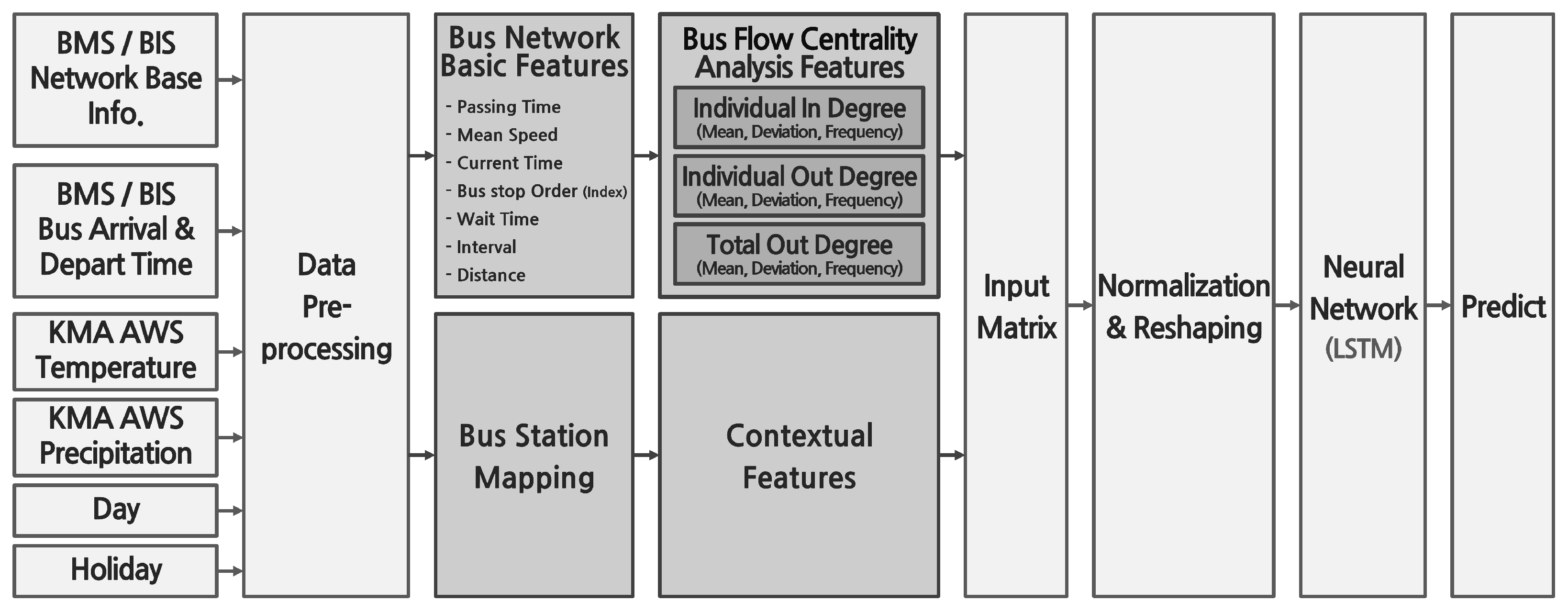
Figure 1 describes the overall flow of our BFC-LSTM modeling approach. First, we retrieve information such as bus network structure and departure/arrival time logs. We obtained these data from BMS (Bus Management System)/BIS (Bus Information System) (the data used in this study cannot be directly disclosed as a matter of ownership. An official request should be made to https://www.open.go.kr/, (accessed on 29 April 2022) for approval of the data acquisition) of Korea. We also collect meteorological data such as temperature and precipitation around every bus stop from systems such as AWS (Automatic Weather System) of KMA (Korea Meteorological Administration) (the data used in this study cannot be directly disclosed as a matter of ownership. An official request should be made to https://data.kma.go.kr/, (accessed on 29 April 2022) for approval of the data acquisition). These data are organized by days, and we denote holiday status. Using interpolation, we fill in missing data due to inspection, omission, and error of the collecting device. After data preprocessing, nine features are extracted through BFC analysis, as explained in Section 3.1.2. We combine BFC-related features and contextual features such as climate information and day of the week, bus location, and its placement order on the route for every bus as an input vector. After normalization and tensor structuring, such a comprehensive feature set is passed through a recurrent neural network. We employed the LSTM algorithm to learn the correlation between the input features and arrival times of buses at every bus stop.

3.1. Feature Extraction

We explain the 26 features of bus traffic: 7 basic features from the bus management systems, 9 features obtained by running BFC analysis, and 10 contextual features around every bus stop.

3.1.1. Bus Network Basic Features

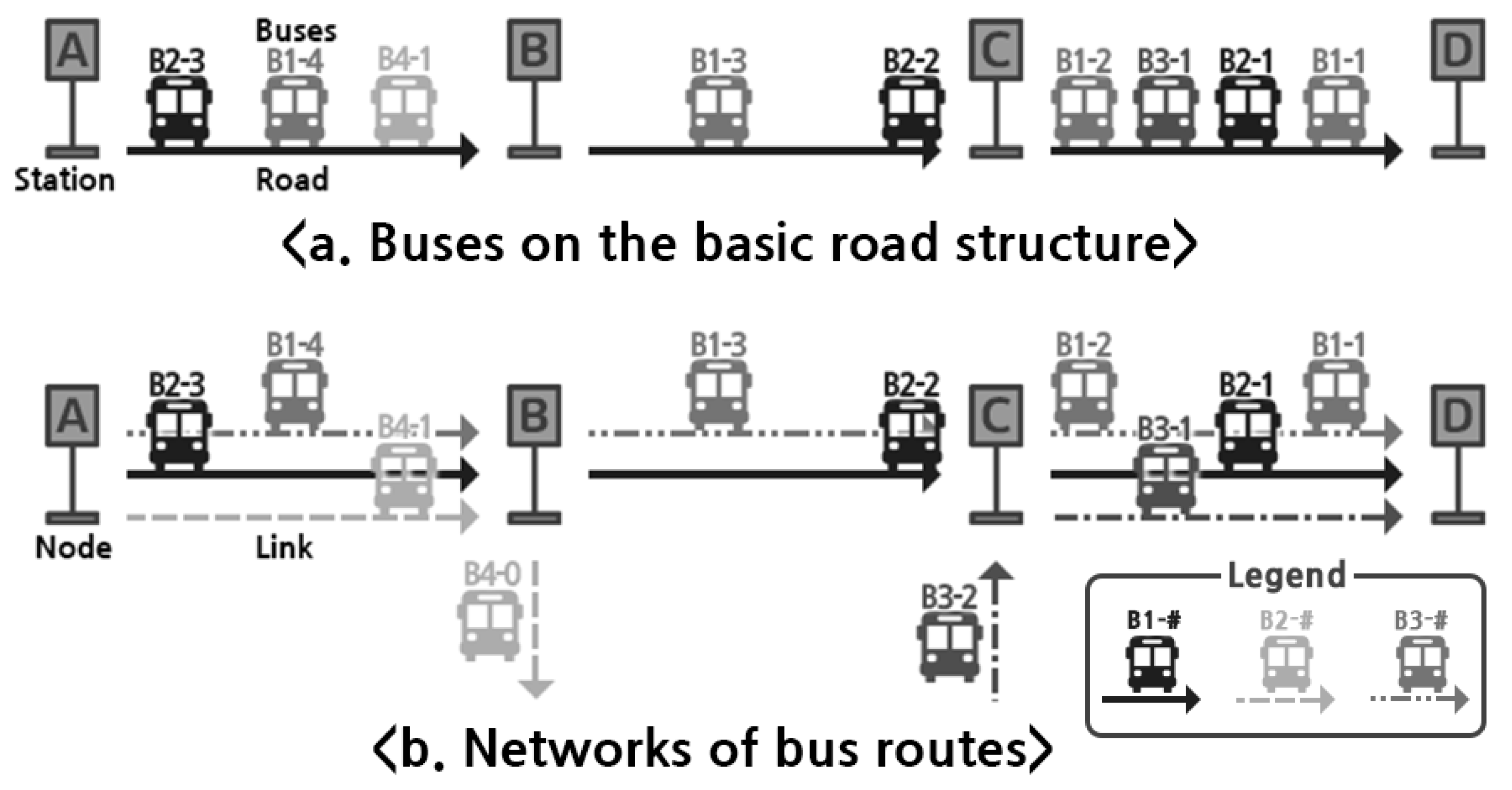
Figure 2a shows a snapshot of the buses en route at a particular time between bus stops. Figure 2b additionally illustrates separate network information per bus route based on the information given on A. The stations are expressed as nodes, and the roads between stations are represented as links. We denote bus routes and buses operating on those routes. For instance, B1-1 and B1-2 are the buses running on bus route B1. By using this information representation, we can recognize how individual bus routes flow in different patterns and which stations and roads can be congested at any point in time.

Note that buses run on the routes strictly in order without overtaking others due to safety regulations. We compute the temporal and ordering characteristics of every bus flow as follows.

• Passing Time $PT$
  $P{T}_{i,j,k}$ is the required time $PT$ in seconds for the jth bus of the route i to arrive at the kth stop from the preceding k− 1th  stop. $PT$ is the difference between arrival time $AT$ and departure time $DT$, as shown in Equation (1). We do not compute starting station’s $PT$ as there is no preceding station.

  $$P{T}_{i,j,k}=A{T}_{i,j,k}-D{T}_{i,j,k-1}$$

  (1)

  For example, as shown in Figure 2, bus B2-2 arriving at stop C is denoted as $A{T}_{B2,2,C}$. The time taken for bus B2-2 to arrive at stop C from stop B can be expressed as $P{T}_{B2,2,C}$. Moreover, the time at which this bus departs from the next stop C can be expressed as $D{T}_{B2,2,C}$.
• Mean Speed $MS$
  Mean Speed $MS$ (m/s) is $PT$ divided by Distance d as shown in Equation (2). Here, d is the distance between stop $k-1$ and stop k on bus route i.

  $$M{S}_{i,j,k}=\frac{P{T}_{i,j,k}}{d_{i,k}}$$

  (2)
• Wait Time $WT$
  Wait Time $WT$ is the amount of time a bus temporarily stays at the bus stop for loading and unloading passengers or a short break, as shown in Equation (3).

  $$W{T}_{i,j,k}=D{T}_{i,j,k}-A{T}_{i,j,k}$$

  (3)
• Inter-Arrival Time I
  Inter-Arrival Time I between buses on a bus route is given in Equation (4). We obtain I by subtracting the time when the j− 1th bus on the bus route i arrived at stop k from the time when the jth bus on i arrived at the same stop.

  $$I_{i,j,k}=A{T}_{i,j,k}-A{T}_{i,j-1,k}$$

  (4)
• Distance d
  Distance d in meters is the Euclidean distance between stops and $k1$ and $k-1$ on bus route i given their coordinates $(x,y)$ as shown in Equation (5).

  $$d_{i,k}=\sqrt{{(d_{i,k_x}-d_{i,k-1_x})}^2+{(d_{i,k_y}-d_{i,k-1_y})}^2}$$

  (5)
• Current Time $CT$
  Current time $CT$ of $AT$ is the time in which the hour, minute, and second information is converted into seconds.
• Bus Stop Order Index
  The Bus Stop Order Index (BSOI) of k denotes the sequential order of station k for bus route i. Each bus route is composed of bus stops in a different order. For instance, in Figure 2, the BSOI of bus stops A, B, C, and D for route B2 are 1, 2, 3, and 4, respectively.

3.1.2. Bus Flow Centrality Analysis Features

BFC (Bus Flow Centrality) analysis is a method of yielding a low-dimensional embedding of spatial flow information from a bus network. As suggested in [8], we selectively embed significant features of the spatial flows on a large-scale bus network into a lower-dimension latent vector to prevent memory outage during training and to save training time. We reduced noise and produced more accurate prediction results by ruling out irrelevant features.

The spatial flow can be characterized by the in-and-out degrees that we have defined as follows.

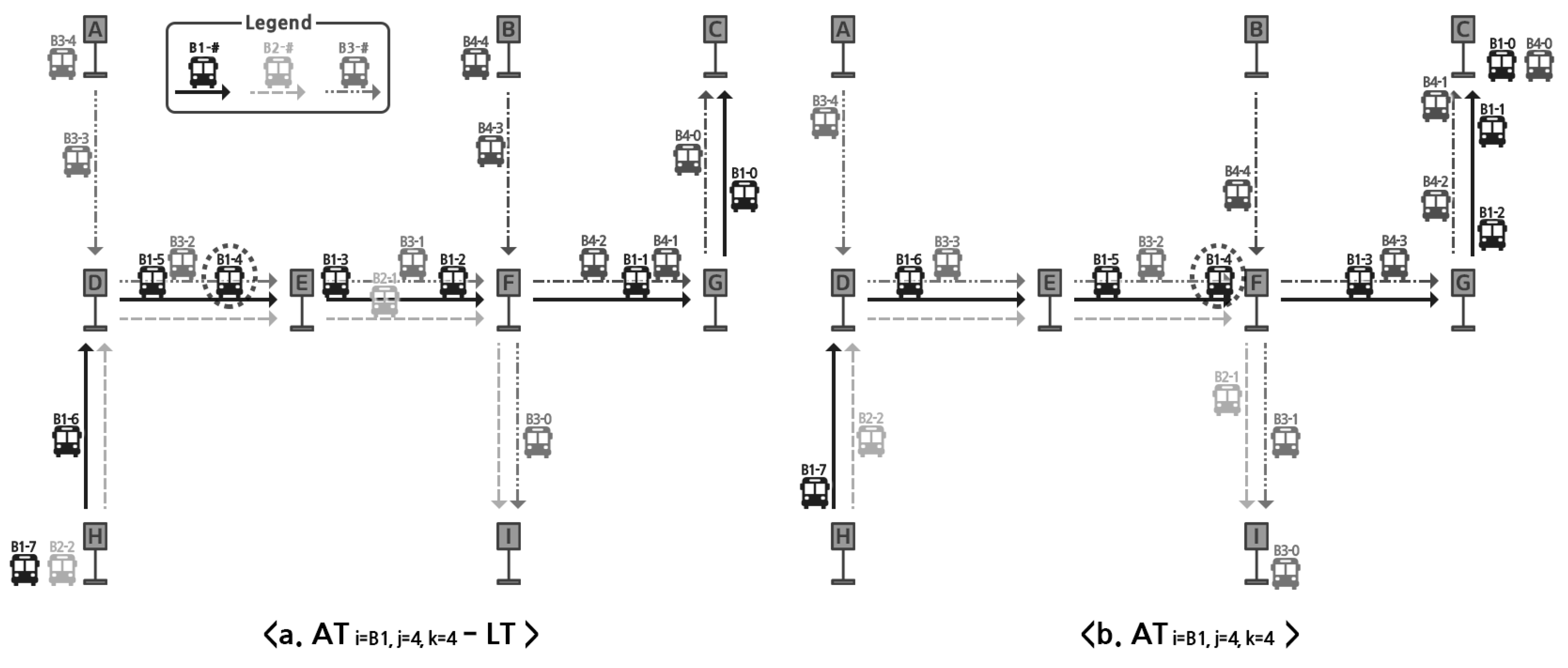
• Individual In Degree $IID$
  $IID$ refers to a set of times buses took to pass a given stop within a certain amount of time to pass through a specific link. Suppose $A{T}_{i,j,k}$ is given. From a preset time period in the past ($LT$) to $A{T}_{i,j,k}$, we retrieve $PT$ of every bus j on route i passing stop k via $k-1$ (denoted as $P{T}_{i,j,k}$). In other words, $II{D}_{i,j,k}$ can be regarded as a set of buses including j and other buses ahead on the same route i that represent the overall inbound spatial flows upon the point when j passes bus station k. The pseudo-code for obtaining $IID$ is presented in Algorithm 1.
  An intuitive example is provided in Figure 3. Bus B1 is en route, passing stops in the order of H, D, E, F, G, and C. Figure 3a,b show a snapshot at $A{T}_{i=B1,j=4,k=4}-LT$ and $A{T}_{i=B1,j=4,k=4}$, respectively, where F is the fourth stop for route $B1$. Bus B1-4 on sub-figure a is in between stops D and E. Later on, sub-figure b shows B1-4 arriving at stop F. In this case, the buses involved in producing $II{D}_{i=B1,j=4,k=4}$ are B1-2, B1-3, and B1-4.
  Spatial flow information is embedded further into a low-dimensional vector. We construct this vector by applying Equations (6)–(8) to a given $IID$. The embedding process is carried out for every stop and every bus. Note that, by using such embedding, we represent not only spatial information but also the different temporal dynamics of every bus on the route.
• Individual Out Degree $IOD$
  $IOD$ represents the outbound spatial flow when a bus j leaves station k for bus stop $k+1$. Suppose $A{T}_{i,j,k}$ is provided. From a preset time period in the past ($LT$) to $A{T}_{i,j,k}$, we retrieve $PT$ of every bus j on route i that left station k for the next stop $k+1$ (denoted as $P{T}_{i,j,k}$). $IOD$ is expected to be another factor for influencing the time a bus takes to reach the next stop. $IOD$ can be obtained by the running the pseudo-code presented in Algorithm 2.
  As shown in Figure 3, buses B1-1 and B1-2 that departed stop G are ahead of B1-4. $PT$ of B1-1 and B1-2 can provide a clue for B1-4 on the condition of the link to the next stop.
  Likewise, $IOD$ is embedded into a latent vector by applying Equations (6)–(8) for every stop and every bus.
• Total Out Degree $TOD$
  $IOD$ is computed for a particular route. On the other hand, $TOD$ is a set of PTs of buses on all routes heading toward the next stop $k+1$ from stations k. $TOD$ represents the aggregate flow pattern on the link to the next stop. Buses not moving to $k+1$ are not considered in constructing $TOD$. For example, in Figure 3, buses on route B3 are not considered for computing $TOD$ for station G via F. It is because the buses on B3 head toward stop I from F instead. Set $TOD$ can be obtained by executing Algorithm 3. $TOD$ is embedded into the latent vector using Equation (6), Equation (7), and Equation (8). Along with $TOD$, we keep IODs separately for all stops and buses to account for microscopic flow patterns that can affect the travel time prediction to the next stations.

  $$NumofSet=\sum _{i\in Set}^{Set}{C}_i$$

  (6)

  $$MeanofSet=\frac{1}{NumofSet}\sum _{i\in Set}^{Set}{x}_i$$

  (7)

  $$DeviationofSet=\sqrt{\frac{1}{NumofSet-1}\sum _{i\in Set}^{Set}{(x_i-\overline{x})}^2}$$

  (8)

Algorithm 1: Individual In Degree $IID$.

Algorithm 2: Individual Out Degree $IOD$.

Algorithm 3: Total Out Degree $TOD$.

3.1.3. Contextual Features

There are ten contextual features in total. First, we obtained the temperature and the precipitation around a bus station. We enumerate the seven days of the week, and we express holidays with a binary value (1 for holidays and 0 for non-holidays). By such enumeration, we can characterize bus passengers’ seasonality and recurring daily travel cycles.

3.2. Models

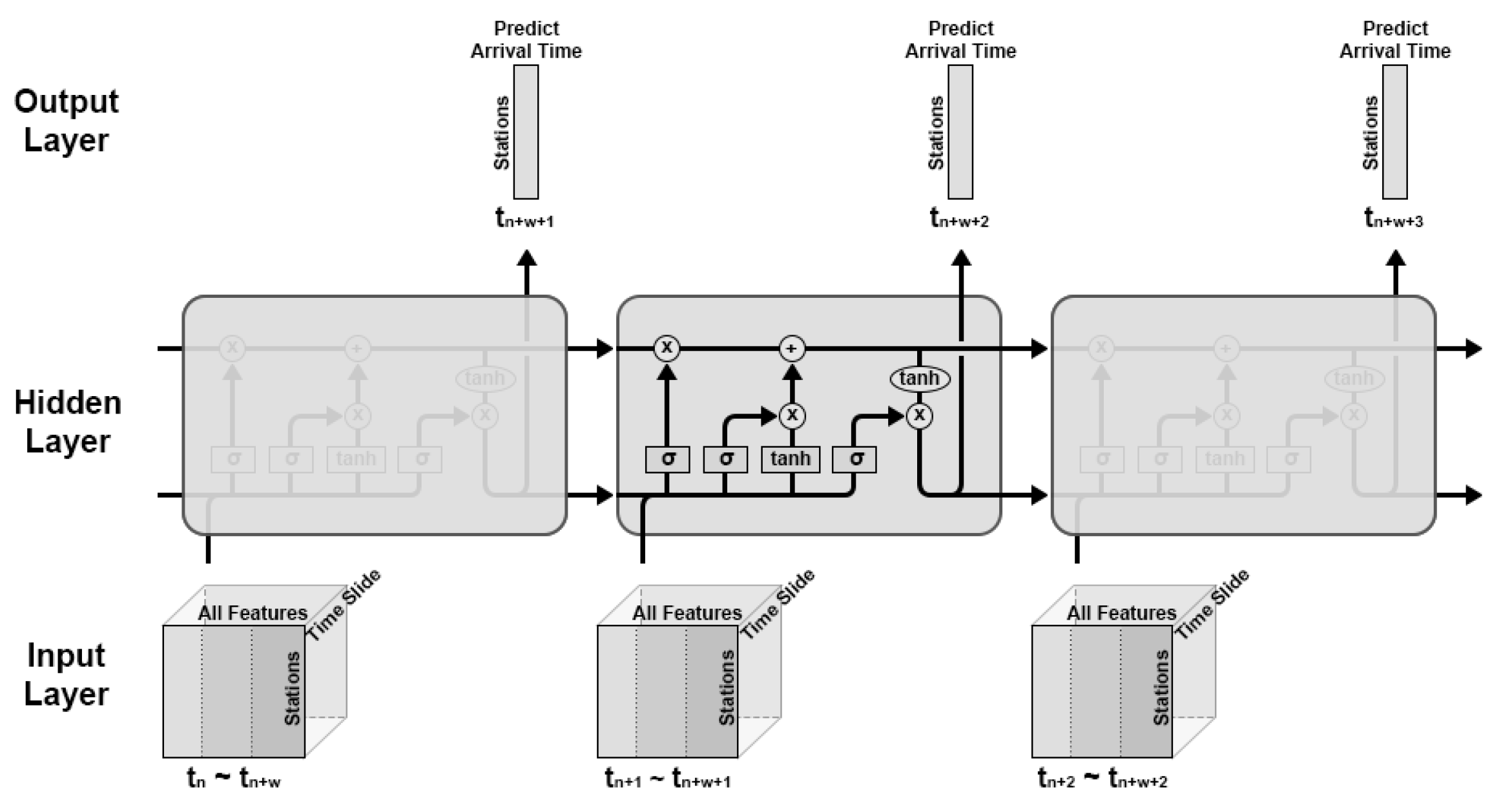
The structure of the input tensor entering the input layer is shown in Figure 4. We combine the basic seven features of the bus mentioned in Section 3.1.1, nine features embedded by using BFC analysis as proposed in Section 3.1.2, and ten contextual features mentioned in Section 3.1.3. The three-dimensional tensor contains the aforementioned composite features generated over multiple past time windows. The tensors flow through the block of hidden layers to output the predicted arrival time at the next station.

The neural network models were configured as follows. We set 128 perceptrons for the LSTM layer with the sigmoid function for the activation at the output layer [42,43]. We used MSE and Adam [44,45] for the loss function and the optimizer, respectively. We set the learning rate to 0.01 and epoch to 100 with the early stoppage option enabled. GRU follows the same parameter setting as LSTM. We added a dense layer of 32 perceptrons relative to LSTM to construct an ALSTM model. The dense layer of ALSTM uses the ReLU function for activation.

We compared the performance of our modeling system against other statistical and deep learning approaches such as Linear Regression [23], Random Forest [24], Multiple Linear Regression [25], ALSTM [11], and GRU [22].

4. Evaluation

The sources for train data were BMS/BIS and AWS of KMA in Korea. BMS/BIS data comprise separate files for each date and bus route. Each BMS/BIS file contains the arrival and departure time logs of the buses on every route. We associated the coordinate of bus stops to extract features, as mentioned in Section 3.1.1. In addition, as mentioned in Section 3.1.2, key features of the bus traffic flows were extracted through BFC analysis. AWS provided precipitation and temperature data around bus stops. We used the data of the buses operating within the Seoul metropolitan area from 00:00:01 on 1 December 2017 to 00:00:00 on 1 January 2018. The attributes of the data are described in

Table 2. Basic bus data attributes.

Data	Status	Time (by Bus Stop ID)	Temperature	Precipitation	Day	Holiday
Mean	-	-	−1.72	0.00	-	-
Median	-	-	−1.7	0.0	-	-
Max	1 (Arrival)	1-January-2018 00:00:00	9.5	1.0	1	1
Min	0 (Depart)	1-December-2017 00:00:00	−16.9	0.0	0	0
Unit	-	DD-MM-YYYY hh:mm:ss	°C	mm	-	-
Time Interval	Each Bus	1-s	1-min	1-min	1-day	1-day
Type	Binary	Int	Float	Float	Binary	Binary

along with basic statistics, units, measurement intervals, and data types. The data were divided into 60% training data, 20% validation data, and 20% test data.

Bus departure and arrival times were interpolated with missing values according to the logic specified in Algorithm 4. There are a few conditions to be aware of, which are listed as follows:

• Buses pass through stops in order;
• A bus x cannot overtake the other bus y ahead if x and y are on the same route;
• Algorithm 4 implements linear interpolation between two points. However, interpolation cannot be carried out for the time intervals, with consecutive nulls appearing at the beginning or end of the sequence.

Interpolation is iteratively performed to keep the spatio-temporal order constraints of the buses. In this case, null values appear at the beginning or end of the sequence, and exception handling is required, such as excluding the bus as not analyzable.

We trained and tested our model on NVIDIA DGX-1 with an 80-core CPU with 160 threads, 8 Tesla V100 GPUs each with 32 GB of exclusive memory, and 512 GB of RAM. NVIDIA DGX-1 is operated with Ubuntu 18.04.5 LTS server, and the machine learning jobs were executed on Docker containers. Machine learning algorithms were implemented with Python (v3.6.9), Tensorflow (v1.15.0), and Keras (v2.3.1) libraries. The following performance indicators were used to measure prediction performance, (1) MAE (Mean Absolute Error) (Equations (9)); (2) RMSE (Root Mean Squared Error) (Equation (10)); (3) MAPE (Mean Absolute Percentage Error) (Equation (11)), as our models conduct regression over continuous arrival time values. We can consider discretizing the time range to intuitively classify punctuality such as “on time” and “late”. The performance of the classifying ML algorithms can be statistically analyzed as presented in [46,47]. Punctuality prediction is an interesting subject for future study.

$$MAE=\frac{1}{n}\sum _{t=1}^n\left|y_t-{\widehat{y}}_t\right|$$

(9)

$$RMSE=\sqrt{\frac{1}{n}\sum _{t=1}^n{(y_t-{\widehat{y}}_t)}^2}$$

(10)

$$MAPE=\frac{1}{n}\sum _{t=1}^n\left|\frac{y_t-{\widehat{y}}_t}{y_t}\right|\ast 100(\%)$$

(11)

Algorithm 4: Interpolation function.

4.1. Measuring Prediction Performance

Prediction models were obtained separately for all bus routes. Experimental results are compiled in

Table 3. Feature usage by modeling methods.

Model	Passing Time Feature	Basic Features	BFC Features	Contextual Features	MAPE (%)
Linear Regression	✓	-	-	-	54.6
Random Forest	✓	-	-	-	20.8
Multi-Linear Regression	✓	✓	✓	-	18.8
			-	-	22.4
LSTM	✓	✓	✓	-	1.19
			✓	✓	2.91
			-	-	31.7
			-	✓	34.9
GRU	✓	✓	✓	-	2.03
			-	-	34.1
ALSTM	✓	✓	✓	-	4.71
			-	-	38.7

. In this paper, we made predictions for 100 buses operating on various routes in Seoul. In short, the LSTM model without contextual features showed the best prediction performance. The source code for BFC analysis and LSTM modeling is available upon request made to the repository at the following link (https://git.apl.hongik.ac.kr/ckswofl/Bus_Arrival_Time_Prediction.git, (accessed on 29 April 2022)).

The Linear Regression model solely relying on passing time information showed poor performance with a MAPE of 54%. The Random Forest, also using passing time information only, performed better than the Linear Regression model with a MAPE of 20.8%. The Multi-Linear Regression model performed similarly to Random Forest with a MAPE of 18.8%. The Multi-Linear Regression model performed well regardless of the contextual features.

Our LSTM consists of 128 perceptrons. We do not use activation functions other than for the LSTM layer. Following this layer, we constructed a fully connected layer with one perceptron to match the shape and the range of the output. For activation [42,43] on the fully connected layer, the sigmoid function was used. For training, the batch size, the epoch, and the time window were set to 10, 200, and 5, respectively. We used Adam [44,45] as an optimizer and configured the learning rate to 0.05. We used MSE for the loss function. With the early stoppage option switched on, we stopped training if no improvement was made in terms of MSE after 20 epochs.

The LSTM model using all the features except contextual information showed a remarkable prediction performance with a MAPE of 1.19%. The MSE values during the training and the validation phases of neural network models with BFC features are as shown in Figure 5. The MSE of the LSTM model converged to the minimum at 60 epochs according. Note that the novel BFC features we defined in this paper boosted performance significantly. Our LSTM model outperformed GRU and ALSTM by showing 40.5% and 74% lower MAPE, respectively.

Several previous studies found the contextual features to improve prediction performance. However, we could not see the benefit of the contextual features in this study. We suspect the reason to be the limited availability of the data. We expect that the train data collected over a more extended period can improve the prediction performance by learning the complex seasonality.

Table 3 shows the feature usage by various modeling approaches. The novel BFC features can be used in any neural network model. We observed significant accuracy improvements when BFC features were used. The LSTM model performed the best with the BFC feature with the lowest MAPE of 1.19%.

Table 4. Performance of BFC-based models against previous non-BFC-based methods in terms of the number of perceptrons in the neural networks.

Number of Perceptrons	Previous Model MAPE (%)			BFC Model MAPE (%)
	LSTM	GRU	ALSTM	LSTM	GRU	ALSTM
64	35.0	37.8	42.8	1.64	2.76	5.87
128	31.7	34.1	39.1	1.19	2.03	4.92
256	32.1	34.3	38.7	1.22	2.11	4.71
512	31.9	34.4	39.0	1.21	2.08	4.74

compares the performance of BFC-based models against non-BFC-based models in terms of number of perceptrons. As mentioned earlier, LSTM with 128 perceptrons and the incorporation of BFC features returned the best result.

4.2. Measuring the Predictive Performance of Random Forest Models

The detailed MAPE results during the training of the Random Forest model are shown in

Table 5. Performance comparison between Random Forest models.

MAPE (%)		T
		25	50	75	100	150	200
D	10	22.08	21.97	21.95	21.93	21.92	21.91
	15	21.29	21.13	21.13	21.03	21.00	20.98
	20	21.25	21.02	21.02	20.90	20.87	20.85
	25	21.23	21.01	21.01	20.89	20.86	20.84
	30	21.26	21.03	21.03	20.91	20.86	20.84
	35	21.24	21.02	21.02	20.90	20.86	20.84

. T is the number of trees in the forest, and D is the maximum allowable depth. Prediction performance improved with larger T and D. However, no further performance improvement was observed at D higher than 25. A large-scale Random Forest could neither capture the complex dynamics of the bus flows nor filter out insignificant data.

4.3. Measuring the Predictive Performance of Multi-Linear Regression Models

The training results of the Multi-Linear Regression model are shown in

Table 6. Performance comparison between Multi-Linear Regression models.

BFC Features LT (min.)	With Contextual Features MAPE (%)	Without Contextual Features MAPE (%)
-	22.41	22.36
5	21.26	21.22
10	20.36	20.35
15	20.03	20.00
20	19.66	19.66
30	19.24	19.23
45	18.92	18.92
60	18.83	18.83
120	18.84	18.84
180	18.84	18.84

. The BFC features did play a role in improving the results. We varied $LT$ as the time window for computing the centrality values, and MAPE was the lowest when $LT$ was set at 60 min. A higher $LT$ value burdens the system as more buses have to be involved in generating $IID$, $IOD$, and $TOD$. This model was not sensitive to context features.

4.4. Measuring the Predictive Performance of LSTM Models

The effect of $LT$ configuration on training results of the LSTM model is shown in

Table 7. The effect of LT and contextual features on LSTM models.

LT (min.)	With Contextual Features			Without Contextual Features
	MAE	RMSE	MAPE (%)	MAE	RMSE	MAPE (%)
5	3.84	8.29	3.71	1.62	4.23	1.65
10	3.09	6.50	3.05	1.15	2.91	1.19
15	2.94	5.75	3.01	1.16	2.92	1.21
20	2.94	5.80	2.98	1.22	2.99	1.26
30	2.88	5.68	2.90	1.32	3.10	1.37
45	3.00	5.80	3.10	1.30	3.12	1.37
60	3.07	5.98	3.09	1.37	3.21	1.42
120	3.08	6.23	3.16	1.43	3.49	1.47
180	3.36	6.51	3.42	1.39	3.25	1.47

. LSTM performed the best when $LT$ was set to 10 without contextual features

Similarly, we observed the effect of the number of past time windows LSTM had to consider. The results are shown in

Table 8. The effect of the number of time windows on LSTM models.

Number of Time Windows	MAE	RMSE	MAPE (%)
5	1.16	2.92	1.19
10	1.33	3.27	1.37
15	1.38	3.38	1.44
20	1.36	3.44	1.40
25	1.42	3.38	1.47

. LSTM performed the best with a relatively small number of time windows. According to BFC, LSTM looking over far-distant past leads to the incorporation of flows of buses that went farther ahead on the route. Those flows do not impact the prediction of the travel time from the current station to the next stop. Therefore, accounting for far-distant bus flows ahead inevitably leads to a higher margin of errors.

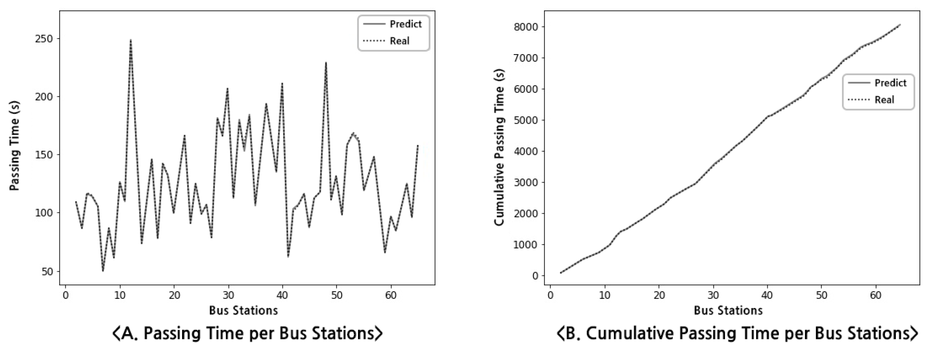
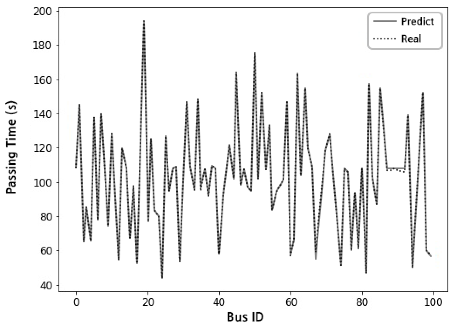
Figure 6A shows the predicted time ($PT$) of a bus on a particular route passes each station. The total travel time of the bus up to the last station is shown in Figure 6B. LSTM makes a highly accurate prediction compared to the actual $PT$ record. Figure 7 shows the predicted time ($PT$) buses on a particular route passing a station in order. Despite the irregularity of the actual $PT$ values between the buses, LSTM modeled without BFC features returned outstanding prediction results.

5. Conclusions

We have presented a novel approach for predicting bus arrival times. In our experiments with actual bus operation data in Seoul, Korea, the short-term spatio-temporal bus flow patterns embedded in a low-dimensional latent vector with BFC analysis helped the LSTM model outperform other renowned recurrent neural network models with an MAE of 1.15 s, an RMSE of 2.91 s, and MAPE of 1.19%. Despite being shorthanded with limited training data availability by BMS/BIT of Korea and the irregularity present in the bus operation patterns, the results were outstanding. The performance of our approach is intriguing as we showed a small margin of error without relying on real-time GPS data.

The enhanced reliability of the bus operators by predictable route plans can attract more travelers leading to a revenue increase. Reduced uncertainty can cut the operation cost by a more efficient deployment plan with respect to buses. Better predictability also helps bus users to reduce travel planning time and cost significantly. Precisely assessing the multilateral economic benefits by using simulations is an interesting subject for a follow-up study.

Despite accurate prediction performance, this study has the following limitations. First, unlike previous studies [8,35,36,37,38], we observed the negative effect of using contextual features. However, we expect the contextual features to take effect when more training data are collected. Second, our solution lacks accountability. We plan to improve accountability by adapting XAI (eXplainable Artificial Intelligence) techniques such as GNN Explainer [48]. As additional future works, we plan to employ GPS data that could further boost accuracy. Utilizing GPS data entails studying the confrontation of the non-negligible costs of collecting and preprocessing GPS. We also plan to experiment with the applicability of our BFC features to more deep learning algorithms such as neural networks with residual learning [49] and Transformer networks with attention layers [50].

References

- Kim, S.; Lewis, M.E.; White, C.C. Optimal vehicle routing with real-time traffic information. IEEE Trans. Intell. Transp. Syst. 2005, 6, 178–188. [Google Scholar] [CrossRef]
- Ying, S.; Yang, Y. Study on vehicle navigation system with real-time traffic information. In Proceedings of the 2008 International Conference on Computer Science and Software Engineering, Wuhan, China, 12–14 December 2008; Volume 4, pp. 1079–1082. [Google Scholar]
- Daganzo, C.; Anderson, P. Coordinating Transit Transfers in Real Time. 2016. Available online: https://escholarship.org/uc/item/25h4r974 (accessed on 29 April 2022).
- Kujala, R.; Weckström, C.; Mladenović, M.N.; Saramäki, J. Travel times and transfers in public transport: Comprehensive accessibility analysis based on Pareto-optimal journeys. Comput. Environ. Urban Syst. 2018, 67, 41–54. [Google Scholar] [CrossRef]
- Kager, R.; Bertolini, L.; Te Brömmelstroet, M. Characterisation of and reflections on the synergy of bicycles and public transport. Transp. Res. Part A Policy Pract. 2016, 85, 208–219. [Google Scholar] [CrossRef] [Green Version]
- Leduc, G. Road traffic data: Collection methods and applications. Work. Pap. Energy Transp. Clim. Chang. 2008, 1, 1–55. [Google Scholar]
- Dafallah, H.A.A. Design and implementation of an accurate real time GPS tracking system. In Proceedings of the The Third International Conference on e-Technologies and Networks for Development (ICeND2014), Beirut, Lebanon, 29 April–1 May 2014; pp. 183–188. [Google Scholar]
- Lee, C.; Yoon, Y. Context-Aware Link Embedding with Reachability and Flow Centrality Analysis for Accurate Speed Prediction for Large-Scale Traffic Networks. Electronics 2020, 9, 1800. [Google Scholar] [CrossRef]
- Treethidtaphat, W.; Pattara-Atikom, W.; Khaimook, S. Bus arrival time prediction at any distance of bus route using deep neural network model. In Proceedings of the 2017 IEEE 20th International Conference on Intelligent Transportation Systems (ITSC), Yokohama, Japan, 16–19 October 2017; pp. 988–992. [Google Scholar]
- Zhou, X.; Dong, P.; Xing, J.; Sun, P. Learning dynamic factors to improve the accuracy of bus arrival time prediction via a recurrent neural network. Future Internet 2019, 11, 247. [Google Scholar] [CrossRef] [Green Version]
- Liu, H.; Xu, H.; Yan, Y.; Cai, Z.; Sun, T.; Li, W. Bus arrival time prediction based on LSTM and spatial-temporal feature vector. IEEE Access 2020, 8, 11917–11929. [Google Scholar] [CrossRef]
- Petersen, N.C.; Rodrigues, F.; Pereira, F.C. Multi-output bus travel time prediction with convolutional LSTM neural network. Expert Syst. Appl. 2019, 120, 426–435. [Google Scholar] [CrossRef] [Green Version]
- Jeong, R.; Rilett, R. Bus arrival time prediction using artificial neural network model. In Proceedings of the 7th International IEEE Conference on Intelligent Transportation Systems (IEEE Cat. No. 04TH8749), Washington, WA, USA, 3–6 October 2004; pp. 988–993. [Google Scholar]
- Lin, W.H.; Zeng, J. Experimental study of real-time bus arrival time prediction with GPS data. Transp. Res. Rec. 1999, 1666, 101–109. [Google Scholar] [CrossRef] [Green Version]
- Gong, J.; Liu, M.; Zhang, S. Hybrid dynamic prediction model of bus arrival time based on weighted of historical and real-time GPS data. In Proceedings of the 2013 25th Chinese Control and Decision Conference (CCDC), Guiyang, China, 25–27 May 2013; pp. 972–976. [Google Scholar]
- Han, Q.; Liu, K.; Zeng, L.; He, G.; Ye, L.; Li, F. A bus arrival time prediction method based on position calibration and LSTM. IEEE Access 2020, 8, 42372–42383. [Google Scholar] [CrossRef]
- Chien, S.I.J.; Ding, Y.; Wei, C. Dynamic bus arrival time prediction with artificial neural networks. J. Transp. Eng. 2002, 128, 429–438. [Google Scholar] [CrossRef]
- Bin, Y.; Zhongzhen, Y.; Baozhen, Y. Bus arrival time prediction using support vector machines. J. Intell. Transp. Syst. 2006, 10, 151–158. [Google Scholar] [CrossRef]
- Yu, B.; Lam, W.H.; Tam, M.L. Bus arrival time prediction at bus stop with multiple routes. Transp. Res. Part Emerg. Technol. 2011, 19, 1157–1170. [Google Scholar] [CrossRef]
- Agafonov, A.; Yumaganov, A. Bus arrival time prediction with lstm neural network. In International Symposium on Neural Networks; Springer: Berlin/Heidelberg, Germany, 2019; pp. 11–18. [Google Scholar]
- Hochreiter, S.; Schmidhuber, J. Long short-term memory. Neural Comput. 1997, 9, 1735–1780. [Google Scholar] [CrossRef]
- Chung, J.; Gulcehre, C.; Cho, K.; Bengio, Y. Empirical evaluation of gated recurrent neural networks on sequence modeling. arXiv 2014, arXiv:1412.3555. [Google Scholar]
- Seber, G.A.; Lee, A.J. Linear Regression Analysis; John Wiley & Sons: Hoboken, NJ, USA, 2012; Volume 329. [Google Scholar]
- Liaw, A.; Wiener, M. Classification and regression by randomForest. R News 2002, 2, 18–22. [Google Scholar]
- Montgomery, D.C.; Peck, E.A.; Vining, G.G. Introduction to Linear Regression Analysis; John Wiley & Sons: Hoboken, NJ, USA, 2021. [Google Scholar]
- Ferris, B.; Watkins, K.; Borning, A. OneBusAway: Results from providing real-time arrival information for public transit. In Proceedings of the SIGCHI Conference on Human Factors in Computing Systems, Atlanta, GA, USA, 10–15 April 2010; pp. 1807–1816. [Google Scholar]
- Zhang, F.; Shen, Q.; Clifton, K.J. Examination of traveler responses to real-time information about bus arrivals using panel data. Transp. Res. Rec. 2008, 2082, 107–115. [Google Scholar] [CrossRef]
- Reinhoudt, E.M.; Velastin, S. A dynamic predicting algorithm for estimating bus arrival time. IFAC Proc. Vol. 1997, 30, 1225–1228. [Google Scholar] [CrossRef]
- Bin, Y.; Zhong-zhen, Y.; Qing-cheng, Z. Bus arrival time prediction model based on support vector machine and kalman filter. China J. Highw. Transp. 2008, 2, 89. [Google Scholar]
- Liu, T.; Ma, J.; Guan, W.; Song, Y.; Niu, H. Bus arrival time prediction based on the k-nearest neighbor method. In Proceedings of the 2012 Fifth International Joint Conference on Computational Sciences and Optimization, Heilongjiang, China, 23–26 June 2012; pp. 480–483. [Google Scholar]
- Suwardo, W.; Napiah, M.; Kamaruddin, I. ARIMA models for bus travel time prediction. J. Inst. Eng. Malays. 2010, 2010, 49–58. [Google Scholar]
- Lingqiu, Z.; Guangyan, H.; Qingwen, H.; Lei, Y.; Fengxi, L.; Lidong, C. A LSTM Based Bus Arrival Time Prediction Method. In Proceedings of the 2019 IEEE SmartWorld, Ubiquitous Intelligence & Computing, Advanced & Trusted Computing, Scalable Computing & Communications, Cloud & Big Data Computing, Internet of People and Smart City Innovation (SmartWorld/SCALCOM/UIC/ATC/CBDCom/IOP/SCI), Leicester, UK, 19–23 August 2019; pp. 544–549. [Google Scholar]
- Panovski, D.; Zaharia, T. Long and Short-Term Bus Arrival Time Prediction With Traffic Density Matrix. IEEE Access 2020, 8, 226267–226284. [Google Scholar] [CrossRef]
- Zhang, K.; Lai, Y.; Jiang, L.; Yang, F. Bus Travel-Time Prediction Based on Deep Spatio-Temporal Model. In International Conference on Web Information Systems Engineering; Springer: Cham, Switzerland, 2020; pp. 369–383. [Google Scholar]
- Kim, D.H.; Hwang, K.Y.; Yoon, Y. Prediction of Traffic Congestion in Seoul by Deep Neural Network. J. Korea Inst. Intell. Transp. Syst. 2019, 18, 44–57. [Google Scholar] [CrossRef]
- Panovski, D.; Zaharia, T. Public transportation prediction with convolutional neural networks. In International Conference on Intelligent Transport Systems; Springer: Cham, Switzerland, 2019; pp. 150–161. [Google Scholar]
- He, P.; Jiang, G.; Lam, S.K.; Tang, D. Travel-time prediction of bus journey with multiple bus trips. IEEE Trans. Intell. Transp. Syst. 2018, 20, 4192–4205. [Google Scholar] [CrossRef]
- Pang, J.; Huang, J.; Du, Y.; Yu, H.; Huang, Q.; Yin, B. Learning to predict bus arrival time from heterogeneous measurements via recurrent neural network. IEEE Trans. Intell. Transp. Syst. 2018, 20, 3283–3293. [Google Scholar] [CrossRef]
- Baimbetova, A.; Konyrova, K.; Zhumabayeva, A.; Seitbekova, Y. Bus Arrival Time Prediction: A Case Study for Almaty. In Proceedings of the 2021 IEEE International Conference on Smart Information Systems and Technologies (SIST), Nur-Sultan, Kazakhstan, 28–30 April 2021; pp. 1–6. [Google Scholar]
- Leong, S.H.; Lam, C.T.; Ng, B.K. Bus Arrival Time Prediction for Short-Distance Bus Stops with Real-Time Online Information. In Proceedings of the 2021 IEEE 21st International Conference on Communication Technology (ICCT), Tianjin, China, 13–16 October 2021; pp. 387–392. [Google Scholar]
- Zhong, G.; Yin, T.; Li, L.; Zhang, J.; Zhang, H.; Ran, B. Bus travel time prediction based on ensemble learning methods. IEEE Intell. Transp. Syst. Mag. 2022, 14, 174–189. [Google Scholar] [CrossRef]
- Nair, V.; Hinton, G.E. Rectified Linear Units Improve Restricted Boltzmann Machines. In Proceedings of the ICML, Haifa, Israel, 21–24 June 2010. [Google Scholar]
- Glorot, X.; Bordes, A.; Bengio, Y. Deep Sparse Rectifier Neural Networks. In Proceedings of the Fourteenth International Conference on Artificial Intelligence and Statistics, Fort Lauderdale, FL, USA, 11–13 April 2011; pp. 315–323. [Google Scholar]
- Kingma, D.P.; Ba, J. Adam: A method for Stochastic Optimization. arXiv 2014, arXiv:1412.6980. [Google Scholar]
- Ruder, S. An Overview of Gradient Descent Optimization Algorithms. arXiv 2016, arXiv:1609.04747. [Google Scholar]
- Nguyen, B.P. Prediction of FMN binding sites in electron transport chains based on 2-D CNN and PSSM Profiles. IEEE/ACM Trans. Comput. Biol. Bioinform. 2019, 18, 2189–2197. [Google Scholar]
- Tng, S.S.; Le, N.Q.K.; Yeh, H.Y.; Chua, M.C.H. Improved Prediction Model of Protein Lysine Crotonylation Sites Using Bidirectional Recurrent Neural Networks. J. Proteome Res. 2021, 21, 265–273. [Google Scholar] [CrossRef]
- Ying, R.; Bourgeois, D.; You, J.; Zitnik, M.; Leskovec, J. GNN explainer: A tool for post-hoc explanation of graph neural networks. arXiv 2019, arXiv:1903.03894. [Google Scholar]
- He, K.; Zhang, X.; Ren, S.; Sun, J. Deep residual learning for image recognition. In Proceedings of the IEEE Conference on Computer Vision and Pattern Recognition, Las Vegas, NV, USA, 27–30 June 2016; pp. 770–778. [Google Scholar]
- Vaswani, A.; Shazeer, N.; Parmar, N.; Uszkoreit, J.; Jones, L.; Gomez, A.N.; Kaiser, Ł; Polosukhin, I. Attention is all you need. In Proceedings of the Advances in Neural Information Processing Systems, Long Beach, CA, USA, 4–9 December 2017; pp. 5998–6008. [Google Scholar]
Figure 1.
The overall procedure for bus flow centrality analysis (BFC) and training for bus arrival time prediction.
Figure 2.
Buses on the basic road structures and the network per bus routes. Symbols A, B, C, and D represent bus stops.
Figure 3.
Snapshot of a sample bus network and snapshot focusing on the bus stop F. Symbols A through I represent bus stops.
Figure 4.
Using LSTM for modeling the correlation between the tensors of comprehensive features and the bus arrival time prediction at every time window.
Figure 5.
MSEs during training and validation.
Figure 6.
Passing times and cumulative passing time of a bus at each bus station.
Figure 7.
Passing times of buses on a station.