
A Hybrid ARIMA-GABP Model for Predicting Sea Surface Temperature
by
 and
and
Xiangyi Chen
1, 
Qinrou Li
1,
Xianghai Zeng
1,
Chuyi Zhang
2,
Guangjun Xu
1,3 and
Guancheng Wang
1,4,* 1
College of Electronic and Information Engineering, Guangdong Ocean University, Zhanjiang 524088, China
2
College of Foreign Languages, Guangdong Ocean University, Zhanjiang 524088, China
3
Southern Marine Science and Engineering Guangdong Laboratory (Zhuhai), Zhuhai 524000, China
4
Shenzhen Institute of Guangdong Ocean University, Shenzhen 518108, China
*
Author to whom correspondence should be addressed.
Electronics 2022, 11(15), 2359; https://0-doi-org.brum.beds.ac.uk/10.3390/electronics11152359
Submission received: 26 June 2022
/
Revised: 25 July 2022
/
Accepted: 26 July 2022
/
Published: 28 July 2022
(This article belongs to the Special Issue Analog AI Circuits and Systems)
Abstract
:Sea surface temperature (SST) is one of the most important parameters in air–sea interaction, and its accurate prediction is of great significance in the study of global climate change. However, SST is affected by heat flux, ocean dynamic processes, cloud coverage, and other factors, which means it contains linear and nonlinear components. Existing prediction models, especially single prediction models, cannot effectively handle these linear and nonlinear components in the meantime, degrading their accuracy concerning the prediction of SST. To remedy this weakness, this paper proposes a novel prediction model by the Lagrange multiplier method to combine the auto-regressive integrated moving average (ARIMA) model and the back propagation (BP) neural network model, where these two models have superior prediction performance for linear and nonlinear components, respectively. Moreover, the genetic algorithm is exploited to construct the genetic algorithm BP (GABP) neural network to further improve the performance of the proposed model. To verify the effectiveness of the proposed model, experiments predicting the SST based on historic time-series data are performed. The experiment results indicate that the mean absolute error (MAE) of the ARIMA-GABP model is only 0.3033 C and the root mean square error (RMSE) is 0.3970 C, which is better than the ARIMA model, BP neural network model, long short-term memory (LSTM) model, GABP neural network model, and ensemble empirical model decomposition BP model among various datasets. Therefore, the proposed model has superior and robust performance concerning predicting SST.
1. Introduction
As the main factor in the interaction between the ocean and the atmosphere, sea surface temperature (SST) plays a significant role in the global climate system [1,2,3,4]. From an environmental point of view, abnormal changes in SST will cause drought, tsunami, and other natural disasters [5]. Regarding the economic aspect, it will cause losses in marine-related fields, such as marine fisheries, fishing ground forecasting, and marine transportation [6,7,8]. To reduce unnecessary losses in the environmental and economic fields, it is vital to predict the SST accurately in advance [6].
At present, many traditional methods have been proposed to predict the time series data like SST [9]. They can be roughly divided into three kinds, numerical prediction method, empirical prediction method, and statistical prediction method [10]. Nishida et al. (2021) used a numerical model for predicting horizontal water temperature distribution in paddy fields [11]. Peeples et al. used empirical prediction to simulate metal accumulation in galaxies [12]. In statistical methods, Rosella Giacometti et al. (2012) compared the Lee–Carter statistical model and used the autoregression-autoregressive conditional heteroskedasticity model to forecast mortality rates [13]. Christiaanse et al. (1971) used the exponential smoothing method to predict the short-term load of the power system [14]. Besides this, the Auto-regressive integrated moving average (ARIMA) model is the most common statistical model used for time series prediction, and can predict the future value of an observed time series. Zheng et al. (2020) employed the ARIMA model to predict total health expenditure in China from 1978 to 2022 [15]. Rosmiati et al. (2021) used the ARIMA technique in determining the ocean climate [16]. The results of it showed that the ARIMA model is very effective in predicting ocean climate phenomena such as EI Niño-Southern Oscillation (ENSO) events. The traditional prediction methods have achieved good prediction results in many fields while the prediction of SST is poor. The SST is easily affected by various factors, such as heat flux, ocean dynamic processes, cloud coverage and so on. Due to the interference of these factors, the time series of SST contains not only the linear components but also the nonlinear components, leading it to change irregularly [17]. When dealing with such complicated SST time series data, these traditional methods cannot fit well with the nonlinear components, which limits their predicting accuracy [10]. Furthermore, the empirical prediction method is conservative, and it is difficult to predict the SST in harsh weather [9].
In recent years, the neural network has become a research hotspot [18,19,20,21]. Prediction methods based on the neural network are efficient and accurate, and can improve the shortcomings of traditional prediction methods. Hou et al. (2017) proposed a gray wolf optimization (GWO)-back propagation (BP) model, and the model can accurately predict the overall trend of cloud server resource load [22]. Guo et al. (2019) predicted Load forecast, which is carried out by using ensemble empirical model decomposition (EEMD)- genetic algorithm BP (GABP) [23]. It can validly realize load forecast, and not only has a higher accuracy but also a stronger stability. He et al. (2021) proposed a novel prediction method based on the empirical model decomposition and gated recurrent unit model [9]. It enjoys an easier training process, faster fitting speed, and higher prediction accuracy. Meng et al. (2021) proposed a gravitational search algorithm BP model that can predict tool wear [24]. The accurate prediction of tool wear is of great significance to reduce machining costs and improve machining efficiency. In addition, Zhang et al. (2017) adopted a long short-term memory (LSTM) neural network to predict SST, which establishes the temporal relationship model of SST to predict future work [25]. The effectiveness of this method is verified by the prediction of the coastal seas of China. Among all the neural network models, the BP neural network is a kind of mature and prevalent prediction model [26,27,28,29]. Since the BP neural network has good nonlinear data fitting ability, it can be widely exploited in various fields [30].
However, regardless of the traditional methods or the neural network-based models, the single model usually has inevitable defects or unreliability. Previous studies have proved that the combination model can obtain the advantages of multiple models, reduce the impact of model defects on prediction values, and overcome the limitations of the single model [26,27,28,29,31]. Xu et al. (2016) proposed a model that conforms to the future change trend of water quality and provides the reference for the related department to predict and protect the Songhua River basin water quality [32]. Zou et al. (2016) proposed the radial basis function (RBF)-BP model to predict the maximum temperature of the concrete pouring storehouse of the high arch dam [33]. The application results of the combined model are accurate, effective, stable, and satisfactory. Wang et al. (2021) proposed a combined model to predict the stability of the high cutting slope [34]. The results show that the prediction accuracy of slope stability by this combined model is better than that by a single model, and the error of the combination model is less than that of a single model. Wang et al. (2021) proposed a combined model that is based on the linear model, shallow neural network, and deep learning to predict wind speed [35]. Compared with the common single model, this model not only fives rise to the prediction accuracy of wind speed but also maintains high stability when the parameters change.
Due to the complexity of the SST, this paper proposes a novel hybrid ARIMA-GABP model that can efficiently fit the linear and nonlinear components in SST. The ARIMA model is a traditional dynamic prediction method, where only the first value is predicted based on the real value, and the next is derived based on the predicted value. This feature degrades its accuracy in long-term prediction, while it has a strong ability to capture the linear relationship [29]. Meanwhile, the BP neural network is superior in predicting nonlinear time series data [36]. Therefore, this paper utilizes the ARIMA model and BP neural network to predict the implicit linear and nonlinear parts of the SST, respectively, and combines them with a Lagrange multiplier. In addition, since the BP neural network has the disadvantages of over-fitting, a slow convergence rate, and falling into the local minimums easily [30,37], the genetic algorithm (GA) is employed to enhance the global search and global optimization ability of the BP neural network so that the hybrid ARIMA-GABP model can have better accuracy.
The contributions of this paper are as follows.
- 1.
- A new combined prediction model, the hybrid ARIMA-GABP is proposed to reduce the prediction error caused by single model defects.
- 2.
- The hybrid model uses the Lagrange multiplier method for weight analysis, taking the advantages of each model.
- 3.
- Compared with various models, the proposed hybrid ARIMA-GABP model has better accuracy in predicting SSTs.
The rest of this paper is constructed as follows. In Section 2, several prevalent prediction models are introduced, e.g., the ARIMA model, BP neural network model, and LSTM model. In Section 3, this paper introduces the genetic algorithm to improve the BP neural network model. Then, the full details of the proposed ARIMA-GABP weight model will unfold. Besides this, simulation experiments of the ARIMA-GABP model and comparison tests of prediction effects with other prediction models are in Section 4. Section 5 draws the conclusions of this paper.
2. Related Works
2.1. ARIMA Model
The ARIMA model, a kind of prevalent time series prediction model proposed by Box and Jenkins [38], was derived from the auto-regressive moving average (ARMA) model. The ARMA model estimates the time series data as
where and denote the auto-regressive coefficient and moving average coefficient, respectively. Moreover, is the white noise sequence, p and q are the orders of the auto-regressive model and the moving average model. To endow the ARMA model with better nonlinear data processing ability, the d-order difference of the primitive non-stationary time series is utilized to construct the ARIMA model, which makes the primitive series stationary and performs the fitting analysis. The flowchart of the ARIMA model is shown in Figure 1. If the primitive series data is non-stationary, d-order difference will be executed to smooth the primitive non-stationary series. Taking a second-order expression as an example, its expression is
where Y denotes the sequence after difference operation. Then, p and q are determined by the Akaike information criterion (AIC) [39] or observed from the auto-correlation and partial auto-correlation.Finally, the ARIMA verifies whether its residual error is white noise. Compare with the ARMA model; the ARIMA model has excellent linear regularity fitting ability and more accurate short-term prediction.
2.2. BP Neural Network
BP neural network is a feed-forward neural network trained by a wide range of error back-propagation algorithms and proposed by Rumelhart and McClelland [40]. The BP neural network can be divided into two parts: data forward transmission and error backward transmission. In the forward-transfer process, the output of each layer is estimated based on the output of the previous layer, the weights, and the bias. If the output of the last layer does not coincide with the expected output, the descent gradient will be distributed in reverse to all units to adjust the weights and thresholds between neurons. By iterating this learning process, the BP neural network can determine parameters corresponding to the minimum error.
The simple structure of the BP neural network is shown in Figure 2a, which consists of input layer, hidden layer, and output layer. The hidden layers can be composed of a single layer or multiple layers [41,42]. Figure 2b demonstrates the flowchart of the BP neural network. Set up input as and output as , and initialize the weights W and V as random values between [0, 1]. After that, the error is
where denotes the actual output and denotes the expected output. Expressing with the parameters of the hidden layer, (3) can be expressed as
where denotes the value of neurons in the hidden layer and denotes the activation function. Furthermore, the error function expressed by the input layer can be formulated as
The weights w and v are continuously adjusted by the gradient descent method to change the connection strength. The error decreases continuously until it reaches its minimum value to find the optimal solution. The process of weight adjustment can be expressed as
2.3. LSTM
In recent years, recurrent neural network (RNN) has had extensive applications in areas such as speech recognition, language modeling, and translation modules. The RNN can predict the future value via historical time series based on a single layer repetition module. However, when the distance between the predicted position and the relevant position increases, the RNN will lose connection of long distance information in long-term prediction [43]. The LSTM is a special RNN neural network model, which replaces the original single repeating module with four kinds of interactive layer repeating modules. Its diagram is shown in Figure 3, demonstrating that the LSTM model is composed of three types of gate, including the forgetting gate (dropping unimportant data information through the forgetting gate), input gate (controlling the number of saved data sample sizes), and output gate (determining the output model value). These three special gates not only enable it to remember long-term memory values but also can discard unimportant information when learning long time series.
3. The Hybrid ARIMA-GABP Model
3.1. GABP Neural Network
The traditional BP neural network algorithm can predict nonlinear data, while it may easily fall into the local optimal solution. Using the genetic algorithm to initialize random weights and thresholds of the BP neural network can relax the shortcomings of being trapped in the local optimal solution and improve the prediction accuracy and efficiency. The GA algorithm seeks the optimal solution by simulating Darwin’s theory of biological evolution [44], which transforms the problem into a cross-mutation process of chromosome genes. It selects the optimal population through chromosome selection, crossover, and mutation operations according to the custom fitness function in the encoding population, and eliminates individuals who are not adapted to the environment. Each generation of chromosomes can inherit the information of the previous generation and make it better than the previous generation. Based on this conception and process, the GA algorithm can avoid the traditional algorithm falling into gradient explosion or local optimal solution so that it finds the global best individual, The GA algorithm process includes data encoding, initializing the population, calculating fitness, selection, chiasma, mutation, and iterating to the optimal solution. The key operation of the GA algorithm is summarized as follows.
- 1.
- Selection: The optimal individual is commonly selected by the roulette wheel, where the higher the relative fitness value , the higher survival probability of the individual. The relative fitness can be estimated aswhere denotes the original fitness value.
- 2.
- Chiasma: The chiasma process can be expressed aswhere and are two different chromosomes and their cross-exchange occurs at the jth element. Besides this, b is a random number from 0 to 1.
- 3.
- Mutation: The mutation of the jth element in chromosome can be expressed aswhere and are the upper and lower boundary of the chromosome , respectively. Moreover, , where T is the iteration number of mutation and is the maximum iteration number of mutation.
After obtaining the optimal individual, the solutions are assigned to the BP neural network as the initial parameter, and thus constitute the GABP model.
3.2. ARIMA-GABP
A single prediction model usually has unavoidable defects or unreliability. By composing different models, the advantages of various models can be integrated, where not only the independent information of each prediction method can be made full use of, but also the impact of the defects of the model itself on the prediction value can be decreased. In addition, the existing studies have indicated that the ARIMA model can highly fit the linear parts of the sequence, and the BP neural network has an excellent ability to process nonlinear data [41,42,45,46]. To improve the prediction accuracy, a hybrid ARIMA-GABP model combining the ARIMA model and GABP model in parallel with Lagrange multiplier method is established. The predicted value of SSTs synthesized by the GABP neural network and ARIMA model are denoted as and , respectively. Moreover, The final predicted value can be defined as
where denotes the weights of the ARIMA model, denotes the weights of the GABP model, and .
The flowchart of the hybrid ARIMA-GABP model is shown in Figure 4, which can be roughly divided into three parts.
- 1.
- The GABP neural network: Based on the seasonal change trend of the monthly average SST data, the data used in the BP neural network are time-shifted by 12 months. Then, the first twelve column matrices are defined as the input layer and the thirteenth row as the output layer. The number of hidden layers in the BP neural network is determined by empirical formula aswhere a and b represent the number of input layers and output layers, respectively. c is a constant between 1 and 10. Then the GA algorithm is employed to optimize the initialization weights and thresholds of the BP neural network. After training, the GABP neural network outputs the predicted SST .
- 2.
- The ARIMA model: Firstly, the ARIMA utilizes the ADF unit-root method to detect the stability of the original SST time series. If p is less than 0.05, the sequence is determined as a stationary series date. Otherwise, the original data should be transformed into stationary time series by d-order difference. Based on the characteristics that the differential operation loses data, the order d should not be large, and equal to 1 or 2 to avoid prediction failure due to data missing.
- 3.
- The Lagrange multiplier: To determine the optimal weight , of the ARIMA model and the GABP neural network, the Lagrange multiplier method takes the minimum error as the optimization objective. Then, the prediction error of the combined model at time t can be expressed aswhere , , , represent the predicted value of the proposed hybrid model, the true value, the predicted value of ARIMA, and the predicted value of GABP neural network, respectively. Moreover, , , denote the error of the proposed hybrid model, the ARIMA model, and the GABP neural network, respectively. Then, determining the weight can be transformed into an optimization problem, which can be formulated asusing the Lagrange multiplier method, the optimal weights are obtained as
4. Simulation
In this section, the hybrid ARIMA-GABP model is exploited to predict the monthly average SST. Moreover, the absolute average error (MAE) and the root mean square error (RMSE) are used to evaluate the accuracy of prediction, which are defined as
where denotes the predicted value and denotes the expected value. The smaller the model’s MAE and RMSE, the higher its accuracy. The simulation environments are summarized as below.
- 1.
- Hardware environment: Intel Core i7-5800H, 16 G running memory, and 1 TB hard disk.
- 2.
- Software environment: Microsoft Windows 11 operating system and MATLAB R2020a.
4.1. Experimental Results of the Hybrid ARIMA-GABP Model
In this section, the implementations of the hybrid ARIMA-GABP model, including data processing, simulation setting, and building block, are described. In addition, the simulative results are also depicted to demonstrate the effectiveness of the proposed model.
4.1.1. Data Prepossessing and Simulation Setting
The data used in this section are the monthly average COBE SSTs from Japan Meteorological Agency (JMA) from the US National Oceanic and Atmospheric Administration (NOAA) (https://psl.noaa.gov/data/gridded/data.cobe.html, accessed on 25 October 2021) from January 1948 to November 2021 in the South China Sea (118.5 E, 22.5 N), which is denoted as . To avoid the interference of outlier data on the experimental results caused by factors such as errors in SST measurement, the isolated forest algorithm is used to remove outlier points and replaces the abnormal month with the average data of the last month and the next month value. Therefore, there are 886 SST data units in this our simulation, which are shown in Figure 5. Then the first average monthly SSTs are set as the training dataset, while the last SSTs are set as the validation dataset to evaluate the accuracy of the predicted models. Furthermore, according to Equations (15) and (16), the weights of the ARIMA and the GABP in the hybrid model are 0.2914 and 0.7086.
4.1.2. Building of the ARIMA Model
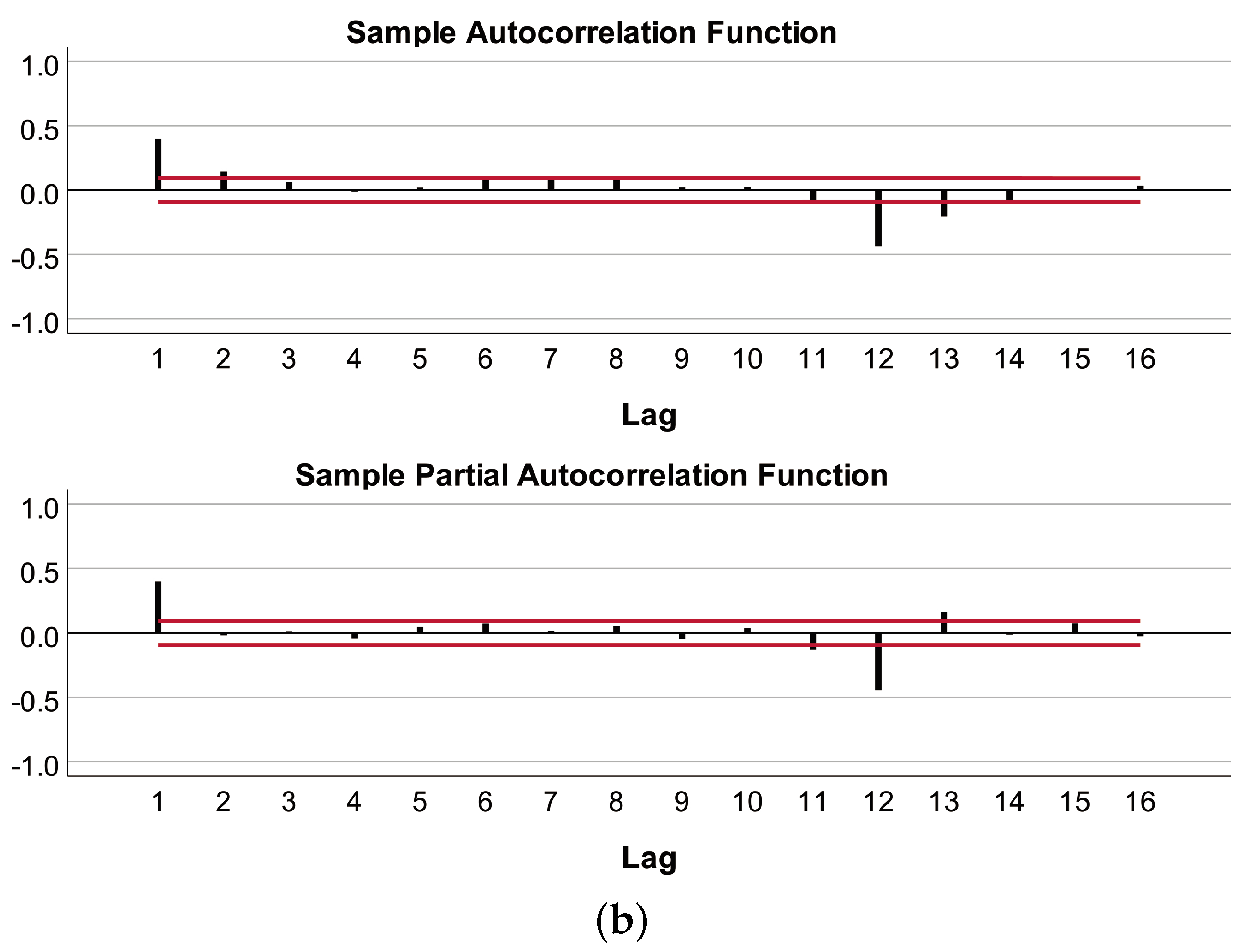
To observe the characteristic of the SSTs, its auto-correlation function (ACF) and partial auto-correlation function (PACF) are depicted in Figure 6, where the black lines denote the correlation at the n-order delay of the ACF and PACF (between −1 and 1), and the red lines represent the boundaries of the 95% confidence interval. According to Figure 5 and Figure 6a, it can be found that the SSTs have obvious seasonal amplitude sinusoidal fluctuation, indicating that the SSTs are unsuitable to apply to the ARIMA model directly. Therefore, the first-order seasonal difference is performed for the SSTs to generate stationary SSTs. The ACF and PACF diagram after difference are shown in Figure 6b, where the periodicity of the SSTs has been eliminated, indicating that the post-difference SSTs are feasible to use in the ARIMA model. Furthermore, according to Figure 6b, p can be 1, 2, 12, and 13, while q can be 1, 11, 12, and 13. Through the enumeration method, the ARIMA model with and can have the best predicted accuracy.
4.1.3. Building of the GABP Model
As discussed before, the monthly average SSTs show a seasonal trend, whose period is twelve months. Therefore, a three-layer GABP neural network is designed to predict the coming SST through the last twelve SSTs. In other words, the input layer of the GABP neural network has twelve neurons, while the output layer has only one neuron. In addition, according to (12), there are eleven neurons in the hidden layer. The training of the GABP neural network includes 1000 steps, where the learning rate is 0.01, the minimum error of the training target is 0.00001, and the activation function is the tansig function, expressed as .
4.1.4. Simulative Results
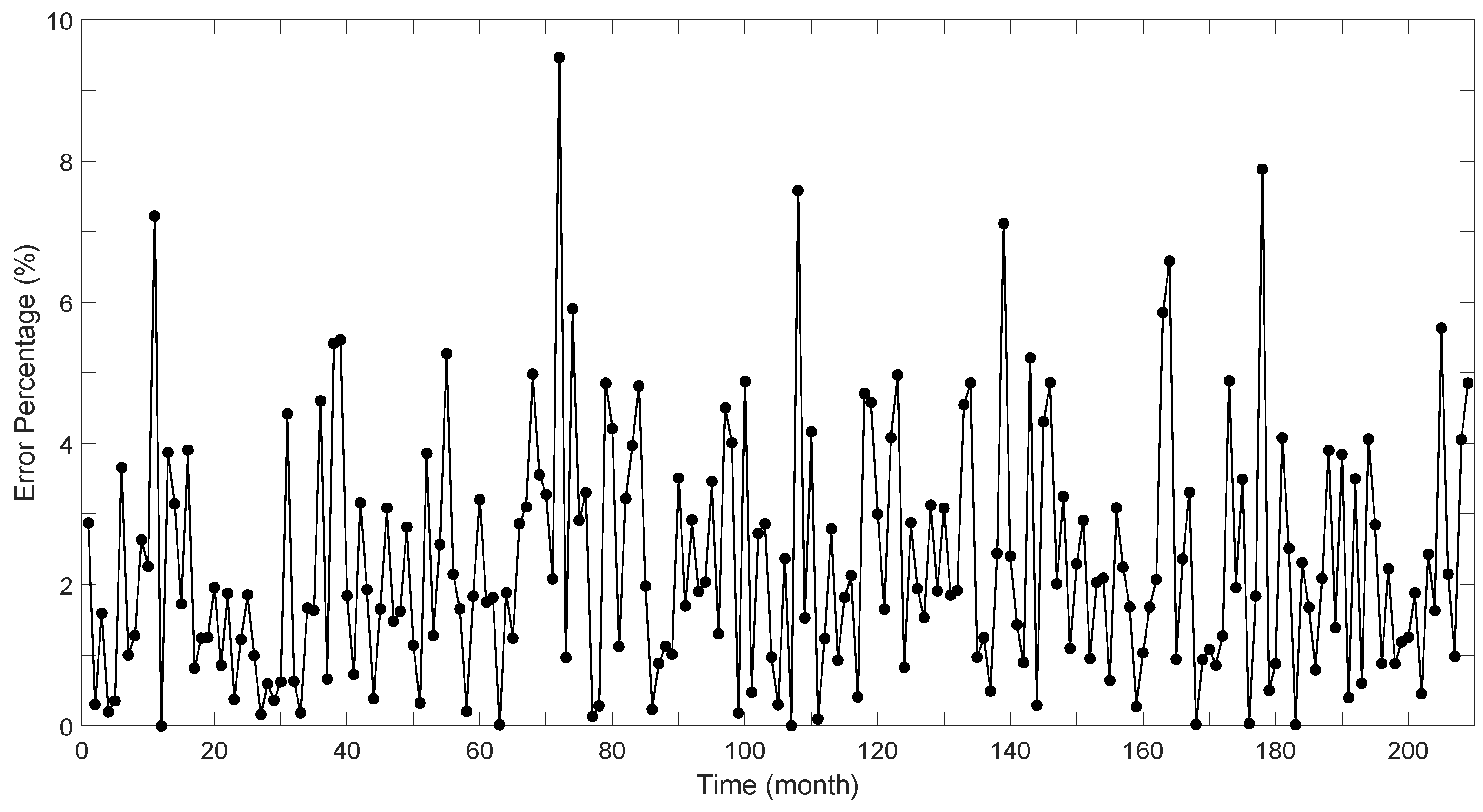
The predicted SSTs synthesized by trained hybrid ARIMA-GABP model are shown in Figure 7, where the black line denotes the predicted SSTs and the dotted lines denote the actual SSTs. In Figure 7, the predicted SSTs almost coincide with the actual one, indicating the high accuracy of the hybrid model. In addition, the error percentage of the prediction is shown in Figure 8, the average error percentage is concentrated around , and the maximum value is below , which also demonstrate the effectiveness of the proposed model.
4.2. Compared Experimental Results
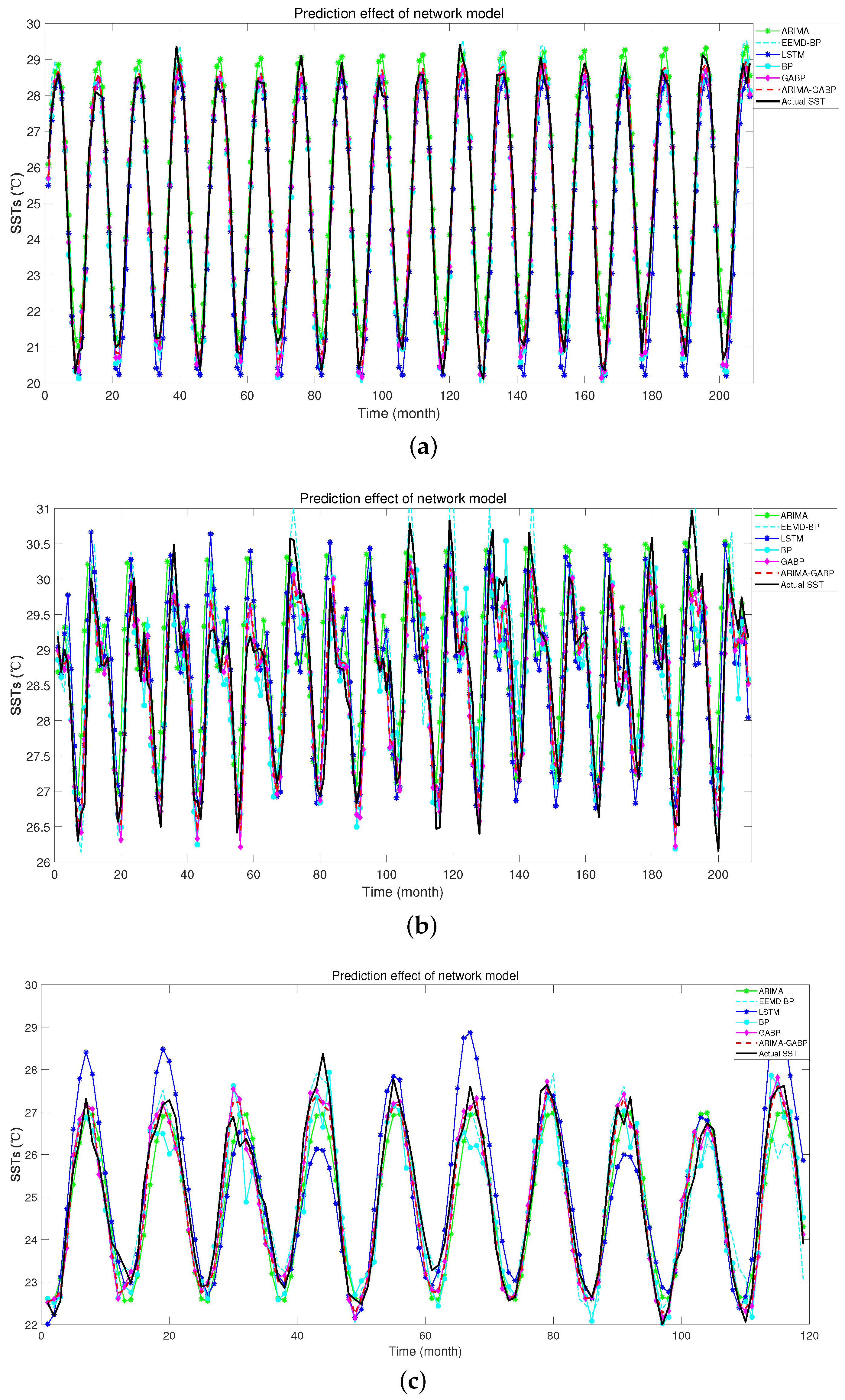
To better illustrate the superiority of the proposed model, several models, including the BP neural network, the ARIMA model, the GABP neural network, the LSTM model [25], and the ensemble empirical model decomposition BP (EEMD-BP) model [4], are also utilized to predict the SSTs for purposes of comparison. Besides this, two more time series SSTs are exploited to evaluate these algorithms, which are denoted as and , respectively. is the average monthly COBE SSTs from December 1981 to July 2022 in the South China Sea (118.5 E 22.5 N) from JMA, while is the SST series of NOAA Optimum Interpolation SST (OISST) V2 from December 1981 to July 2022 in the South China Sea (118.5 E 22.5 N). Furthermore, (, ) in the hybrid ARIMA-GABP model regarding these two datasets are (0.1953, 0.8046) and (0.3152, 0.6876), respectively.
The predicted SSTs versus the ground-truth SSTs are shown in Figure 9. According to Figure 9, the BP neural network and the ARIMA model cannot effectively predict the SSTs of and , while the LSTM model achieves the worst accuracy with . Among three datasets, the GABP model, the EEMD-BP model, and the hybrid ARIMA-GABP model can efficiently predict the SSTs, whose plots of the SSTs can effectively track the trajectory of the ground-true SSTs. In addition, to directly evaluate the accuracy, Table 1 summarized the MAE and RMSE of these models with various datasets. Among these models, the hybrid ARIMA-GABP model achieves the lowest MAE and RMSE (denoted in bold font) with all datasets, demonstrating the robustness of the hybrid ARIMA-GABP model against datasets. Furthermore, compared with the single model, i.e., the ARIMA model and the GABP model, the proposed hybrid ARIMA-GABP model can improve the predicted accuracy efficiently, verifying the feasibility of the design discipline proposed in this paper.
5. Conclusions
This paper proposed a hybrid ARIMA-GABP model to combine the advantages of the ARIMA model in linear prediction and the BP neural network in nonlinear prediction through the Lagrange multiplier method. To verify the validity and effeteness of the proposed model, this paper utilized historic SSTs in various datasets to train and validate the proposed model. The simulating results demonstrate that the proposed model can predict the SSTs successfully with 0.3033 C MAE and 0.3970 C RMSE. Moreover, compared with the BP model, the ARIMA model, the LSTM model, the GABP model, and the EEMD-BP model, this hybrid model achieved best prediction accuracy among various datasets, verifying the superiority of the hybrid model. Applying this method to more areas or developing the improved hybrid model will be subjects of our future work.
Author Contributions
Conceptualization, G.W.; methodology, X.C. and X.Z.; software, X.C.; validation, X.C. and G.W.; writing—original draft preparation, X.C., C.Z. and Q.L.; writing—review and editing, G.W. and G.X.; project administration, G.W.; funding acquisition, G.W. All authors have read and agreed to the published version of the manuscript.
Funding
This research was funded by Southern Marine Science and Engineering Guangdong Laboratory (Zhuhai) (SML2020SP007); National Undergraduate Training Program for Innovation and Entrepreneurship Training Project (202110566030); and First Class Discipline Construction Platform Project in 2019 of Guangdong Ocean University (231419026).
Data Availability Statement
Not applicable.
Acknowledgments
The authors would like to thank the anonymous reviewers and editors for their valuable comments and suggestions on earlier versions of the manuscript.
Conflicts of Interest
The authors declare no conflict of interest.
References
- Zhu, L.; Liu, Q.; Liu, X.; Zhang, Y. RSST-ARGM: A Data-Driven approach to long-term sea surface temperature prediction. EURASIP J. Wirel. Commun. Netw. 2021, 1, 171. [Google Scholar] [CrossRef]
- Xiao, C.; Chen, N.; Hu, C.; Wang, K.; Chen, Z. Short and mid-term sea surface temperature prediction using time-series satellite data and LSTM-AdaBoost combination approach. Remote Sens. Environ. 2019, 233, 111358. [Google Scholar] [CrossRef]
- Karim, M.R. Seasonal ARIMA for forecasting sea surface temperature of the north zone of the Bay of Bengal. Res. Rev. J. Stat. 2013, 2, 23–31. [Google Scholar]
- Wu, Z.; Jiang, C.; Conde, M.; Deng, B.; Chen, J. Hybrid improved empirical mode decomposition and BP neural network model for the prediction of sea surface temperature. Ocean Sci. 2019, 15, 349–360. [Google Scholar] [CrossRef] [Green Version]
- Fang, Y.W.; Tang, Y.M.; Li, J.D.; Liu, T. Several statistical models to predict tropical indian ocean sea surface temperature anomaly. J. Mar. Sci. 2018, 36, 1–15. [Google Scholar]
- Hou, S.; Li, W.; Liu, T.; Zhou, S.; Guan, J.; Qin, R.; Wang, Z. D2cl: A dense dilated convolutional LSTM model for sea surface temperature prediction. IEEE J. Sel. Top. Appl. Earth Obs. Remote Sens. 2021, 14, 12514–12523. [Google Scholar] [CrossRef]
- Cheng, Z.; Tang, C.; Cai, B.; Shen, D. Influencing factors of SST variation along the south china coast during 1960–2013. Trop. Geogr. 2016, 36, 906–914. [Google Scholar]
- Wang, X.X.; Shao, L.M.; Cao, X.C. Climatic characteristics study of the sea fog evolution in the western yellow sea from 2005 to 2007. Mar. Forecast. 2012, 29, 62–68. [Google Scholar]
- He, Q.; Hu, Z.Y.; Xu, H.F.; Song, W.; Du, Y.L. SST prediction method based on EMD-GRU model. Laser Optoelectron. Prog. 2021, 58, 342–350. [Google Scholar]
- He, Q.; Cheng, Z.; Sun, M.; Jiang, X.Y.; Qi, F.M.; Huang, D.M.; Song, W. Surface temperature parallel prediction algorithm under spark platform. Mar. Sci. Bull. 2019, 38, 280–289. [Google Scholar]
- Nishida, K.; Yoshida, S.; Shiozawa, S. Numerical model to predict water temperature distribution in a paddy rice field. Agric. Water Manag. 2021, 245, 106553. [Google Scholar] [CrossRef]
- Peeples, M.S.; Somerville, R.S. An empirical prediction for stellar metallicity distributions in nearby galaxies. Mon. Not. R. Astron. Soc. 2013, 428, 1766–1773. [Google Scholar] [CrossRef] [Green Version]
- Giacometti, R.; Bertocchi, M.; Rachev, S.T.; Fabozzi, F.J. A comparison of the Lee–Carter model and AR–ARCH model for forecasting mortality rates. Insur. Math. Econ. 2012, 50, 85–93. [Google Scholar] [CrossRef]
- Christiaanse, W.R. Short-term load forecasting using general exponential smoothing. IEEE Trans. Power Appar. Syst. 1971, 2, 900–911. [Google Scholar] [CrossRef]
- Zheng, A.; Fang, Q.; Zhu, Y.; Jiang, C.; Wang, X. An application of ARIMA model for predicting total health expenditure in china from 1978–2022. J. Glob. Health 2020, 10, 010803. [Google Scholar] [CrossRef] [PubMed]
- Rosmiati, R.; Liliasari, S.; Tjasyono, B.; Ramalis, T.R. Development of ARIMA technique in determining the ocean climate prediction skills for pre-service teacher. J. Phys. Conf. Ser. 2021, 1731, 012072. [Google Scholar] [CrossRef]
- Lu, X.T.; Sun, Y.; Da, L.L.; Xu, G.J. Prediction of seawater temperature time series based on EMD. Ocean Technol. 2009, 28, 79–82. [Google Scholar]
- Wang, G.; Hao, Z.; Zhang, B.; Jin, L. Convergence and robustness of bounded recurrent neural networks for solving dynamic Lyapunov equations. Inf. Sci. 2022, 588, 106–123. [Google Scholar] [CrossRef]
- Wang, G.; Huang, H.; Yan, J.; Cheng, Y.; Fu, D. An integration-implemented Newton-raphson iterated algorithm with noise suppression for finding the solution of dynamic Sylvester equation. IEEE Access 2020, 8, 34492–34499. [Google Scholar] [CrossRef]
- Liu, M.; Chen, L.; Du, X.; Jin, L.; Shang, M. Activated gradients for deep neural networks. IEEE Trans. Neural Netw. Learn. Syst. 2021, 1–13. [Google Scholar] [CrossRef]
- Jin, L.; Wei, L.; Li, S. Gradient-based differential neural-solution to time-dependent nonlinear optimization. IEEE Trans. Autom. Control 2022. [Google Scholar] [CrossRef]
- Hou, K.; Guo, M.; Li, X.; Zhang, H. Research on optimization of GWO-BP Model for cloud server load prediction. IEEE Access 2021, 9, 162581–162589. [Google Scholar] [CrossRef]
- Guo, W.; Jiang, X.Y.; Luo, Y.; Han, Q. Short-term load forecasting in a certain area based on EEMD-GABP. Electr. Power Eng. Technol. 2019, 38, 93–98. [Google Scholar]
- Meng, X.; Zhang, J.; Xiao, G.; Chen, Z.; Yi, M.; Xu, C. Tool wear prediction in milling based on a GSA-BP model with a multisensor fusion method. Int. J. Adv. Manuf. Technol. 2021, 114, 3793–3802. [Google Scholar] [CrossRef]
- Zhang, Q.; Wang, H.; Dong, J.; Zhong, G.; Sun, X. Prediction of sea surface temperature using long short-term memory. IEEE Geosci. Remote Sens. Lett. 2017, 14, 1745–1749. [Google Scholar] [CrossRef] [Green Version]
- Cheng, W.; Zhou, Y.; Guo, Y.; Hui, Z.; Cheng, W. Research on prediction method based on ARIMA-BP combination model. In Proceedings of the 3rd International Conference on Electronic Information Technology and Computer Engineering (EITCE 2019), Xiamen, China, 18–20 October 2019; IEEE: Piscataway, NJ, USA, 2019; pp. 663–666. [Google Scholar]
- Chen, C.J.; Nie, X.C.; Zhang, J. Prediction of tunnel pressure wave for high-speed train based on arma model. China Meas. Test 2013, 39, 5–9. [Google Scholar]
- Zhu, C.; Zhang, J.; Liu, Y.; Ma, D.; Li, M.; Xiang, B. Comparison of GA-BP and PSO-BP neural network models with initial BP model for rainfall-induced landslides risk assessment in regional scale: A case study in Sichuan, China. Nat. Hazards 2020, 100, 173–204. [Google Scholar] [CrossRef]
- Yang, H.; Li, X.; Qiang, W.; Zhao, Y.; Zhang, W.; Tang, C. A network traffic forecasting method based on SA optimized ARIMA-BP neural network. Comput. Netw. 2021, 193, 108102. [Google Scholar] [CrossRef]
- Liu, Y.; Dai, J.; Zhao, S.; Zhang, J.; Li, T.; Zheng, Y.C.; Shang, W.; Wang, Z. A bidirectional reflectance distribution function model of space targets in visible spectrum based on GA-BP network. Appl. Phys. B 2020, 126, 114. [Google Scholar] [CrossRef]
- Han, J.; Pei, J.; Kamber, M. Data Mining: Concepts and Technique, 3rd ed.; Elsevier: Waltham, MA, USA, 2011. [Google Scholar]
- Xu, M.; Yan, F.; Liu, Z.; Li, G.; Qu, P. Forecasting of water quality using grey GM (1,1)-wavelet-GARCH hybrid method in Songhua River Basin. Trans. Chin. Soc. Agric. Eng. 2016, 32, 137–142. [Google Scholar]
- Zou, H.; Zhou, Y.H.; Wang, L.; Zhang, Z.Y. Maximum temperature prediction of concrete pouring storehouse of high arch dam based on RBF-BP neural network model. Water Resour. Power 2016, 34, 67–69. [Google Scholar]
- Wang, P.F. Study on stability prediction of high cutting slope based on GM-RBF combination model. Build. Struct. 2021, 51, 140–145. [Google Scholar]
- Wang, S.; Wang, J.; Lu, H.; Zhao, W. A novel combined model for wind speed prediction–Combination of linear model, shallow neural networks, and deep learning approaches. Energy 2021, 234, 121275. [Google Scholar] [CrossRef]
- Wang, X. Research on the prediction of per capita coal consumption based on the ARIMA–BP combined model. Energy Rep. 2022, 8, 285–294. [Google Scholar] [CrossRef]
- Liu, C.; Ling, J.C.; Kou, L.; Chou, L.; Wu, J.Q. Performance comparison between GA-BP neural network and BP neural network. Chin. J. Health Stat. 2013, 30, 173–176. [Google Scholar]
- Box, G. Box and Jenkins: Time Series Analysis, Forecasting and Control; Palgrave Macmillan: London, UK, 2013; pp. 161–215. [Google Scholar]
- Biswas, R.; Bhattacharyya, B. ARIMA modeling to forecast area and production of rice in West Bengal. J. Crop Weed 2013, 9, 26–31. [Google Scholar]
- Van Ooyen, A.; Nienhuis, B. Improving the convergence of the back-propagation algorithm. Neural Netw. 1992, 5, 465–471. [Google Scholar] [CrossRef]
- Cybenko, G.V. Approximation by superpositions of a sigmoidal function. Anal. Theory Appl. 1993, 5, 17–28. [Google Scholar]
- Hornik, K.; Stinchcombe, M.; White, H. Multilayer feedforward networks are universal approximators. Neural Netw. 1989, 2, 359–366. [Google Scholar] [CrossRef]
- Di, H.; Zhao, X.J.; Zhang, Z.L. Research on commodity futures investment strategy based on LSTM adaboost model. South. Financ. 2018, 8, 62–76. [Google Scholar]
- Holland, J.H. Genetic algorithms. Sci. Am. 1992, 267, 66–73. [Google Scholar] [CrossRef]
- Babu, C.N.; Reddy, B.E. A moving-average filter based hybrid ARIMA–ANN model for forecasting time series data. Appl. Soft Comput. 2014, 23, 27–38. [Google Scholar] [CrossRef]
- Büyükşahin, Ü.Ç.; Ertekin, Ş. Improving forecasting accuracy of time series data using a new ARIMA-ANN hybrid method and empirical mode decomposition. Neurocomputing 2019, 361, 151–163. [Google Scholar] [CrossRef] [Green Version]
Figure 1.
The flowchart of the auto-regressive integrated moving average (ARIMA) model.

Figure 2.
(a) The simple structure of the back propagation (BP) neural network. (b) The flowchart of the BP neural network.
Figure 2.
(a) The simple structure of the back propagation (BP) neural network. (b) The flowchart of the BP neural network.

Figure 3.
The diagram of the long short-term memory (LSTM) model.

Figure 4.
The flowchart of the hybrid ARIMA-genetic algorithm BP (GABP) model.

Figure 5.
The series of the sea surface temperatures (SSTs) from 1948 to 2021.

Figure 6.
(a) the auto-correlation function (ACF) and partial auto-correlation function (PACF) diagram of the raw SSTs. (b) the ACF and PACF diagram of the SSTs after difference.
Figure 6.
(a) the auto-correlation function (ACF) and partial auto-correlation function (PACF) diagram of the raw SSTs. (b) the ACF and PACF diagram of the SSTs after difference.


Figure 7.
The predicted SSTs of the hybrid ARIMA-GABP model and the actual SSTs in the test set.

Figure 8.
The error percentage of the prediction in the test set.

Figure 9.
The predicted SSTs synthesized by various methods versus ground-truth SSTs. (a) The stimulative results with . (b) The stimulative results with . (c) The stimulative results with .
Figure 9.
The predicted SSTs synthesized by various methods versus ground-truth SSTs. (a) The stimulative results with . (b) The stimulative results with . (c) The stimulative results with .


Table 1.
The absolute average error (MAE) and the root mean square error (RMSE) among various methods and various datasets.
Table 1.
The absolute average error (MAE) and the root mean square error (RMSE) among various methods and various datasets.
| Metrics | |||||||
|---|---|---|---|---|---|---|---|
| Models | MAE (C) | RMSE (C) | MAE (C) | RMSE (C) | MAE (C) | RMSE (C) | |
| ARIMA | 0.4831 | 0.5904 | 0.6484 | 0.8507 | 0.4564 | 0.5483 | |
| BP | 0.4466 | 0.5540 | 0.4019 | 0.4985 | 0.5895 | 0.7798 | |
| LSTM [25] | 0.4354 | 0.5377 | 0.5105 | 0.6517 | 0.6632 | 0.8418 | |
| GABP | 0.3503 | 0.4450 | 0.3253 | 0.4029 | 0.3279 | 0.4564 | |
| EEMD-BP [4] | 0.3587 | 0.4508 | 0.3746 | 0.5988 | 0.3628 | 0.4209 | |
| Ours | 0.3221 | 0.4058 | 0.3152 | 0.3970 | 0.3033 | 0.4029 | |
Publisher’s Note: MDPI stays neutral with regard to jurisdictional claims in published maps and institutional affiliations. |
© 2022 by the authors. Licensee MDPI, Basel, Switzerland. This article is an open access article distributed under the terms and conditions of the Creative Commons Attribution (CC BY) license (https://creativecommons.org/licenses/by/4.0/).
Share and Cite
MDPI and ACS Style
Chen, X.; Li, Q.; Zeng, X.; Zhang, C.; Xu, G.; Wang, G. A Hybrid ARIMA-GABP Model for Predicting Sea Surface Temperature. Electronics 2022, 11, 2359. https://0-doi-org.brum.beds.ac.uk/10.3390/electronics11152359
AMA Style
Chen X, Li Q, Zeng X, Zhang C, Xu G, Wang G. A Hybrid ARIMA-GABP Model for Predicting Sea Surface Temperature. Electronics. 2022; 11(15):2359. https://0-doi-org.brum.beds.ac.uk/10.3390/electronics11152359
Chicago/Turabian StyleChen, Xiangyi, Qinrou Li, Xianghai Zeng, Chuyi Zhang, Guangjun Xu, and Guancheng Wang. 2022. "A Hybrid ARIMA-GABP Model for Predicting Sea Surface Temperature" Electronics 11, no. 15: 2359. https://0-doi-org.brum.beds.ac.uk/10.3390/electronics11152359
Note that from the first issue of 2016, this journal uses article numbers instead of page numbers. See further details here.