A Hierarchical Estimation Method for Road Friction Coefficient Combining Single-Step Moving Horizon Estimation and Inverse Tire Model

Abstract

To improve the real-time performance of the estimation method of road friction coefficient (RFC) based on moving horizon estimation (MHE), a hierarchical estimation method for RFC combining single-step MHE (S-MHE) and inverse tire model (ITM) based on lateral vehicle dynamics is proposed in this study. Firstly, a hierarchical estimation framework is designed to decouple vehicle and tire systems. Secondly, the S-MHE estimator is designed based on the nonlinear vehicle model to estimate the lateral tire force. Thirdly, the ITM is deduced based on the Pacejka model, and the estimator for the RFC based on the ITM is designed. Finally, the estimation accuracy, convergence speed, and real-time performance of the proposed method and the traditional MHE method are compared and discussed through different tests based on CarSim and Simulink. The results show that compared with the traditional MHE method, the proposed method reduces the average computation time to about 0.125 s and improves the real-time performance by more than 30% while ensuring the estimation accuracy and convergence speed.

1. Introduction

Road traffic injuries are the eighth cause of global death and a global health threat [1]. Scholars have studied and analyzed various factors that lead to vehicle crashes and found that nearly a quarter of crashes occurred in rainy, snowy, or foggy weather and occurred on icy, snowy, or wet roads [2]. In addition, relevant research also shows that the collision frequency of vehicles on wet roads is twice that on dry roads [3]. The main cause of this accident is the driver’s lack of accurate evaluation of the road friction coefficient (RFC), which results in driving behavior/maneuvering beyond the friction limit of the tire [4].

In recent years, the use of advanced driver assistance systems (ADAS) and autonomous driving technologies to improve road safety and reduce traffic accidents, especially reducing vehicle crashes in extreme weather conditions, is a topic that has been widely discussed and researched [5,6,7]. The performance of these systems or technologies, such as adaptive cruise control (ACC), lateral collision avoidance, automatic emergency braking (AEB), path planning, and tracking control, often relies on accurate road friction coefficients [8,9,10]. Therefore, the estimation of RFC has always been an important issue in the field of vehicle control.

Scholars classify the estimation methods of RFC into two types: sensor-based and vehicle dynamics-based [11]. The former usually uses special sensors such as optical sensors, visual sensors, acoustic sensors, and tire tread sensors to identify RFC [4]. On the one hand, the high cost of these off-board sensors limits the application of such methods in production vehicles. On the other hand, the recognition accuracy of such methods is easily disturbed by the external environment [12]. Therefore, in recent years, methods based on vehicle dynamics have been increasingly favored by scholars [11].

The estimation method of RFC based on vehicle dynamics can be further subdivided into the longitudinal slip-based method and lateral slip-based method. The representative methods of the former include methods based on slip-slope curves (including friction coefficient-slip curves) [13,14,15,16] and longitudinal dynamics models [9,17,18]. Since there is no significant difference in the longitudinal stiffness of the tires on the rigid pavement with low and high friction in the low longitudinal excitation condition, the longitudinal stiffness of the tires generally requires large excitation to obtain accurate identification results [11,19]. On the other hand, studies have shown that the longitudinal stiffness or slip-slope of a tire is very sensitive to changes in tire parameters, such as tire pressure or tread depth (meaning tire wear) and temperature conditions [20,21]. Therefore, it is difficult for the estimation method of RFC based on longitudinal slip to produce satisfactory estimation results under normal driving conditions with small longitudinal excitation. This means that the longitudinal slip-based method is insufficient to achieve ADAS and autonomous driving [8].

The lateral slip-based estimation methods for RFC mainly include methods using the tire self-aligning torque model [22,23] and the lateral dynamics model [24,25]. Due to the high sensitivity of tire self-aligning torque to the change of RFC, the estimation method based on tire self-aligning torque can realize the estimation of RFC at a lower excitation level [26]. However, such methods require modeling of suspension and steering systems. Although the electric power steering (ESP) system provides the total axle alignment torque, the estimation of the tie self-aligning torque needs to take into account the moment components generated by the mechanical trail. Compensation for these moment components significantly complicates such estimation method [8]. Compared with the method based on tire self-aligning torque, the lateral dynamics model-based method has higher practicability. Meanwhile, at low excitation levels, lateral dynamics also show higher sensitivity of friction coefficient than longitudinal dynamics. Therefore, methods based on lateral dynamics show greater potential in the estimation of FRC. Table 1 shows the summary of different estimation methods based on vehicle dynamics.

In terms of estimation algorithms, particle filter (PF), Kalman filter (KF) and its variants, and moving horizon estimation (MHE) have been widely studied and applied [26,27,28]. Some studies have demonstrated that MHE performs better among the above methods [28,29,30]. MHE is an optimization-based algorithm that uses finite measurements in the past to solve an optimal estimation [9]. The main advantage of MHE is that it can directly deal with the estimation problem of complex nonlinear dynamic systems with constraints [27,30]. In view of the highly nonlinear dynamics of vehicles, more and more scholars suggest using MHE to estimate vehicle state and road friction coefficient [9,31,32]. Table 2 shows the summary of several estimation algorithms mentioned above.

However, the online rolling optimization mechanism of MHE is computationally expensive, especially for strongly nonlinear systems such as vehicle-tire dynamics. This huge computational burden may cause the estimation system to fail to meet the high real-time requirements of vehicle control. Therefore, a hierarchical estimation method of RFC based on single-step MHE (S-MHE) and inverse tire model (ITM) is proposed in this study. The main contributions of this study are as follows. (1) A hierarchical estimation framework is proposed to decouple vehicle and tire dynamics and reduce the complexity of the optimization problem. (2) An MHE estimation algorithm based on a single-step optimization strategy is designed to realize the estimation of variables that are not system states. (3) An ITM-based RFC estimator that only requires forward calculation is designed to improve real-time performance.

This paper is organized as follows. Section 2 introduces the overall framework of the proposed hierarchical estimation method. Section 3 establishes the vehicle and tire dynamics models. Section 4 introduces the design details of the estimator combining S-MHE and ITM and the traditional MHE estimator. Section 5 provides test results under different conditions. This study is summarized in Section 6.

Table 1. Summary of different estimation methods based on vehicle dynamics.

Literature	Method	Features
[13,14,15,16,20,21]	Slip-slope curves or friction coefficient-slip curves	1. Computationally inexpensive. 2. Large excitations are usually required to achieve accurate identification results. 3. Sensitive to changes in tire parameters.
[17,18]	Longitudinal dynamics models	1. Large excitations are usually required to achieve accurate identification results. 2. Sensitive to changes in tire parameters.
[22,23,26]	Tire self-aligning torque model	1. High sensitivity to RFC. 2. Modeling of suspension and steering systems is required. 3. Low practicability.
[24,25]	Lateral dynamics model	1. High sensitivity to RFC. 2. High practicability.

Table 1. Summary of different estimation methods based on vehicle dynamics.

Literature	Method	Features
[13,14,15,16,20,21]	Slip-slope curves or friction coefficient-slip curves	1. Computationally inexpensive. 2. Large excitations are usually required to achieve accurate identification results. 3. Sensitive to changes in tire parameters.
[17,18]	Longitudinal dynamics models	1. Large excitations are usually required to achieve accurate identification results. 2. Sensitive to changes in tire parameters.
[22,23,26]	Tire self-aligning torque model	1. High sensitivity to RFC. 2. Modeling of suspension and steering systems is required. 3. Low practicability.
[24,25]	Lateral dynamics model	1. High sensitivity to RFC. 2. High practicability.

Table 2. Summary of common estimation algorithms.

Literature	Method	Features
[11,13,17,18,22,26,28]	Kalman filter and its variant	1. Applicable to linear and unconstrained systems subject to normal distribution. 2. Computationally inexpensive.
[27,30]	Particle filter	1. Applicable to non-Gaussian and non-linear systems. 2. Particle degeneracy and the curse of dimensionality problems exist.
[9,25,28,29,30,32]	Moving horizon estimation	1. Applicable to linear or non-linear, constrained or unconstrained systems. 2. High computational costs

Table 2. Summary of common estimation algorithms.

Literature	Method	Features
[11,13,17,18,22,26,28]	Kalman filter and its variant	1. Applicable to linear and unconstrained systems subject to normal distribution. 2. Computationally inexpensive.
[27,30]	Particle filter	1. Applicable to non-Gaussian and non-linear systems. 2. Particle degeneracy and the curse of dimensionality problems exist.
[9,25,28,29,30,32]	Moving horizon estimation	1. Applicable to linear or non-linear, constrained or unconstrained systems. 2. High computational costs

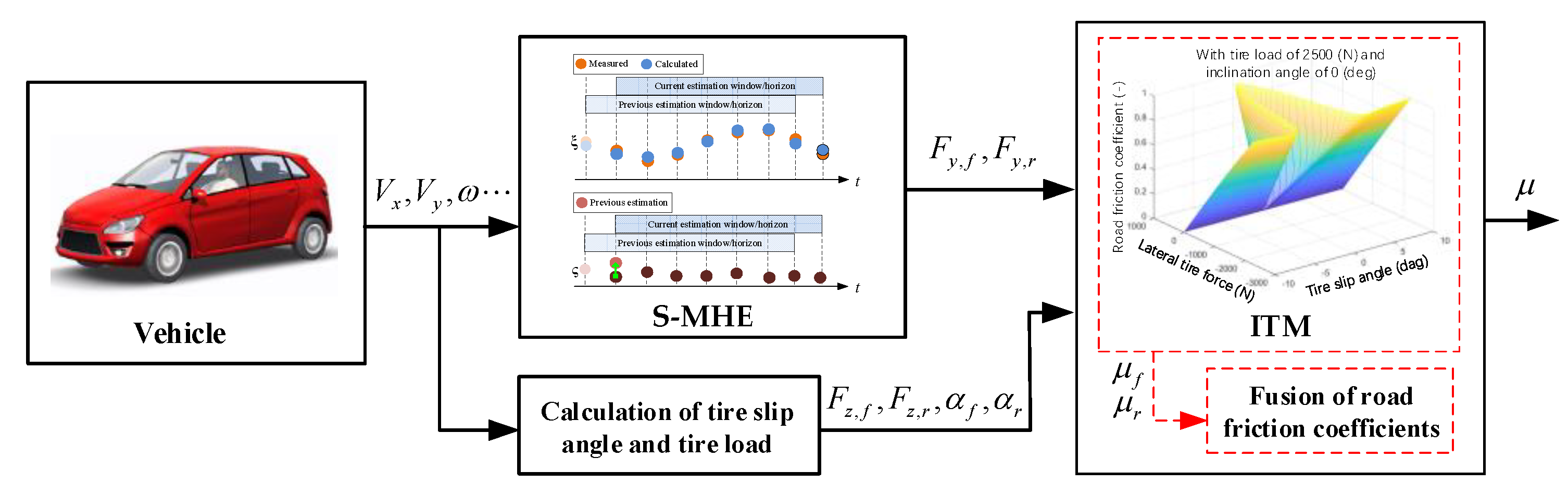
2. Overall Structure of Hierarchical Estimation Method

The vehicle-tire dynamic system is a complex, non-linear system, and the RFC estimation problem based on the above system is computationally complex. In this study, vehicle dynamics and tire dynamics are decoupled, and a hierarchical RFC estimation method is designed. The RFC estimation problem based on vehicle-tire dynamics is decomposed into a tire force estimation problem based on the vehicle model and an RFC estimation based on the inverse tire model so that the complexity of the optimization problem is greatly reduced. The overall structure of the proposed estimation method is shown in Figure 1. S-MHE is the upper estimator, which is responsible for estimating the lateral tire force. The ITM-based lower estimator estimates the RFC based on the lateral tire force estimated by S-MHE.

3. Vehicle and Tire Dynamics Models

The vehicle model used in this study is the single-track vehicle dynamics model, also known as the bicycle model, which will be used to design the tire force estimator based on S-MHE. The model only focuses on the lateral motion and yaw motion of the vehicle while assuming that the input of the vehicle is the front steering angle, as shown in Figure 2.

Table 3. Symbols used in the vehicle model.

Symbol	Description	Symbol	Description
Vx	Longitudinal speed	${\delta }_f$	Front steering angle
Vy	Lateral speed	Fy,f	Lateral tire force on the front tire
$\omega$	Vehicle yaw rate	Fy,r	Lateral tire force on the rear tire
${\alpha }_f$	Front tire slip angle	lf	Distance between front axle and CoG
${\alpha }_r$	Rear tire slip angle	lr	Distance between rear axle and CoG

shows the symbols used in the vehicle model.

The lateral motion and yaw motion of the vehicle can be described as:

$$\begin{array}{l}m{a}_y=F_{y,f}\cos {\delta }_f+F_{y,r}\\ I_z\dot{\omega }=l_f{F}_{y,f}\cos {\delta }_f-l_r{F}_{y,r}\end{array}$$

(1)

where $m$ indicates vehicle mass, $I_z$ means vehicle yaw moment of inertia, $a_y$ denotes the lateral acceleration.

The RFC estimator based on ITM depends on a high-precision tire model. To accurately describe the complex nonlinear characteristics of the tire system, especially the relationship between RFC and tire force, the Pacejka tire model is adopted in this study. The lateral force expression given by the Pacejka 5.2 model is as follows [33]:

$$F_y=F_{y0}(\alpha ,\gamma ,\mu ,F_z)$$

(2)

$$F_{y0}=D_y\sin [C_y\arctan \{B_y{\alpha }_y-E_y(B_y{\alpha }_y-\arctan (B_y{\alpha }_y))\}]+S_{Vy}$$

(3)

$${\alpha }_y=\alpha +S_{Hy}$$

(4)

$${\gamma }_y=\gamma {\lambda }_{\gamma y}$$

(5)

$$C_y=p_{Cy1}{\lambda }_{Cy}$$

(6)

$$D_y={\mu }_y{F}_z{\zeta }_2$$

(7)

$${\mu }_y=(p_{Dy1}+p_{Dy2}d{f}_z)(1-p_{Dy3}{\gamma }_y^2)\mu$$

(8)

$$E_y=(p_{Ey1}+p_{Ey2}d{f}_z)\{1-(p_{Ey3}+p_{Ey4}{\gamma }_y)\mathrm{sgn}({\alpha }_y)\}{\lambda }_{Ey},\mathrm{with}{E}_y\le 1$$

(9)

$$K_{y0}=p_{Ky1}{F}_{z0}\sin [2\arctan \{\frac{F_z}{p_{Ky2}{F}_0{\lambda }_{Fz0}}\}]{\lambda }_{F_{z0}}{\lambda }_{Ky}$$

(10)

$$K_y=K_{y0}(1-p_{Ky3}\left|{\gamma }_y\right|){\zeta }_3$$

(11)

$$B_y=K_y/(C_y{D}_y)$$

(12)

$$S_{Hy}=(p_{Hy1}+p_{Hy2}d{f}_z){\lambda }_{Hy}+p_{Hy3}{\gamma }_y{\zeta }_0+{\zeta }_4-1$$

(13)

$$S_{Vy}=F_z\{(p_{Vy1}+p_{Vy2}d{f}_z){\lambda }_{Vy}+(p_{Vy3}+p_{Vy4}d{f}_z){\gamma }_y\}\mu {\zeta }_4$$

(14)

$$K_{y\gamma 0}=P_{Hy3}{K}_{y0}+F_z(p_{Vy3}+p_{Vy4}d{f}_z)$$

(15)

$$d{f}_z=\left(F_z-F_{z,0}{\lambda }_{Fz0}\right)/\left(F_{z,0}{\lambda }_{Fz0}\right)$$

(16)

where $\gamma$ represents the inclination angle, which is assumed to be zero in this study to simplify the model. $\mu$ represents the RFC. $F_z$ denotes the tire load. The tire load and tire slip angle at the front and rear tires are calculated as

$$\begin{array}{l}{F}_{z,f}=\frac{mg}{\left(l_f+l_r\right)}\left(l_r-\frac{h_g{\dot{V}}_x}{g}\right)\\ F_{z,r}=\frac{mg}{\left(l_f+l_r\right)}\left(l_f+\frac{h_g{\dot{V}}_x}{g}\right)\end{array}\}$$

(17)

$$\begin{array}{l}{\alpha }_f=\frac{V_y+\omega \cdot l_f}{V_x}-{\delta }_f\\ {\alpha }_r=\frac{V_y-\omega \cdot l_r}{V_x}\end{array}\}$$

(18)

Table 4. The key parameters used in the tire model.

Symbol	Value	Symbol	Value
$p_{Cy1}$	1.29	$p_{Ky2}$	1.72
$p_{Dy1}$	−0.9	$p_{Ky3}$	0.22
$p_{Dy2}$	0.18	$p_{Hy1}$	0.0035
$p_{Dx3}$	−4.5	$p_{Hy2}$	−0.003
$p_{Ey1}$	−1.07	$p_{Hy3}$	0.045
$p_{Ey2}$	0.68	$p_{Vy1}$	0.045
$p_{Ey3}$	−0.63	$p_{Vy2}$	−0.03
$p_{Ey4}$	−12.35	$p_{Vy3}$	−0.174
$p_{Ky1}$	−12.95	$p_{Vy4}$	−0.45
${\zeta }_0$	1	${\zeta }_3$	1
${\zeta }_2$	1	${\zeta }_4$	1
${\lambda }_{F_{z0}}$	1	${\lambda }_{Ky}$	1
${\lambda }_{Cy}$	2	${\lambda }_{Hy}$	0
${\lambda }_{Ey}$	1	${\lambda }_{Vy}$	0
${\lambda }_{\gamma y}$	1	$F_0$	4100

shows the key parameters used in the tire model. These parameters have been matched with the tires in CarSim.

4. Design of Estimators

This section mainly consists of three parts, detailing the design details of the traditional MHE-based RFC estimator, the S-MHE-based tire force estimator, and the ITM-based RFC estimator.

4.1. MHE-Based RFC Estimator

MHE is an estimation method based on optimization; the estimation problem is solved repeatedly at each sampling time. As Figure 3 shown, MHE minimizes the errors between the finite sequence of measurements in the past and the output sequence of the model to solve the optimal estimation, which corresponds to the moment of the first value of the sequence of measurements. After obtaining the optimal solution, it is re-substituted into the system model, and an iterative calculation is performed to obtain the estimated value required at the current moment. In the next step, the latest measurements will be considered, and the second element in the estimation sequence in the previous step will be taken as the initial state for the new estimation variables.

Taking yaw rate and lateral acceleration as system outputs, which can be easily obtained from the sensor, according to Equation (1), the estimation equation of MHE can be obtained:

$$\begin{array}{l}\dot{\varsigma }\left(t\right)=f\left(\varsigma \left(t\right)\right)+v\left(t\right)\\ \mathsf{\xi }\left(t\right)=h\left(\varsigma \left(t\right)\right)\end{array}$$

(19)

where state variables $\varsigma =\mu$, system output $\mathsf{\xi }={[a_y,\omega ]}^T$, $v$ is system disturbance. In addition,

$$\begin{array}{l}f\left(\varsigma \right)=\dot{\varsigma }\\ h\left(\varsigma \right)=\left(\begin{array}{l}\left(F_{y,f}\cos {\delta }_f+F_{y,r}\right)/m\\ {\displaystyle \int \left(\left(l_f{F}_{y,f}\cos {\delta }_f-l_r{F}_{y,r}\right)/I_z\right)}dt\end{array}\right)\end{array}$$

In this study, it is assumed that $\dot{\mathsf{\varsigma }}=0$.

Through the Runge–Kutta method, the above estimating equation is discretized, and the discrete estimating equation is

$$\begin{array}{l}\varsigma \left(k+1\right)=f\left(\varsigma \left(k\right)\right)+v\left(k\right)\\ \mathsf{\xi }\left(k\right)=h\left(\varsigma \left(k\right)\right)\end{array}$$

(20)

At time T, the latest N measurement can be expressed as

$${\left\{\tilde{\mathsf{\xi }}\left(k\right)\right\}}_{T-N}^{T-1}=\{\tilde{\mathsf{\xi }}\left(T-N\right),\tilde{\mathsf{\xi }}\left(T-N+1\right),\cdots \tilde{\mathsf{\xi }}\left(T-1\right)\}$$

(21)

The N disturbance before time T can be expressed as

$${\left\{v\left(k\right)\right\}}_{T-N}^{T-1}=\{v\left(T-N\right),v\left(T-N+1\right),\cdots v\left(T-1\right)\}$$

(22)

The cost function of the traditional MHE estimator can be defined as

$$\begin{array}{r}{J}_{MHE}\left(\left\{v\left(k\right)\right\},\varsigma \left(T-N\right)\right)={\displaystyle \sum _{k=T-N}^{T-1}{\Vert \tilde{\mathsf{\xi }}\left(k\right)-\mathsf{\xi }\left(k\right)\Vert }_{{\mathrm{\Gamma }}_{\mathsf{\xi }}}^2}\\ +{\Vert v\left(k\right)\Vert }_{{\mathrm{\Gamma }}_v}^2+{\Vert \varsigma \left(T-N\right)-\overline{\varsigma }\left(T-N\right)\Vert }_{{\mathrm{\Gamma }}_{\varsigma }}^2\end{array}$$

(23)

where $\overline{\varsigma }\left(T-N\right)$ refers to the second element of the estimation sequence in the previous step. At the initial moment, it can also be considered as an a priori estimate of the estimated variable. ${\mathrm{\Gamma }}_{\mathsf{\xi }}$, ${\mathrm{\Gamma }}_{\varsigma }$ and ${\mathrm{\Gamma }}_v$ refer to the weight coefficients.

Finally, the estimation problem of the traditional MHE can be described as

$$\begin{array}{l}\underset{\left\{v\left(k\right)\right\},\varsigma \left(T-N\right)}{\min }{J}_{MHE}\left(\left\{v\left(k\right)\right\},\varsigma \left(T-N\right)\right)\\ s.t.\\ \{\begin{array}{l}\varsigma \left(k+1\right)=f\left(\varsigma \left(k\right)\right)+v\left(k\right)\\ \mathsf{\xi }\left(k\right)=h\left(\varsigma \left(k\right)\right)\end{array}\\ \hspace{1em}\hspace{1em}{\varsigma }_{\min }\le \varsigma \left(k\right)\le {\varsigma }_{\max }\\ \hspace{1em}\hspace{1em}{\mathsf{\xi }}_{\min }\le \mathsf{\xi }\left(k\right)\le {\mathsf{\xi }}_{\max }\end{array}$$

(24)

where ${\varsigma }_{\min }={\mu }_{\min }=0$, ${\varsigma }_{\max }={\mu }_{\max }=1$, ${\mathsf{\xi }}_{\min }={\left[-{\mu }_{\max }g,-{\mu }_{\max }g/V_x\right]}^T$ and ${\mathsf{\xi }}_{\max }=[{\mu }_{\max }g,$ ${{\mu }_{\max }g/V_x]}^T$.

The above optimization problem is solved by the “active set” method. The current value of the estimated variable can be obtained by substituting the solution $(\left\{v\left(k\right)\right\},\varsigma \left(T-N\right))$ into Equation (20) and calculating iteratively.

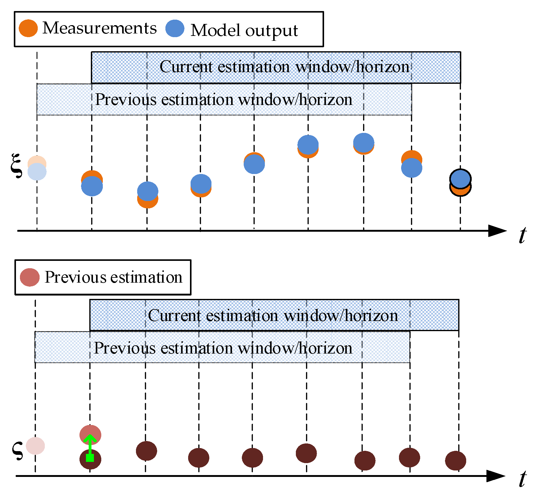
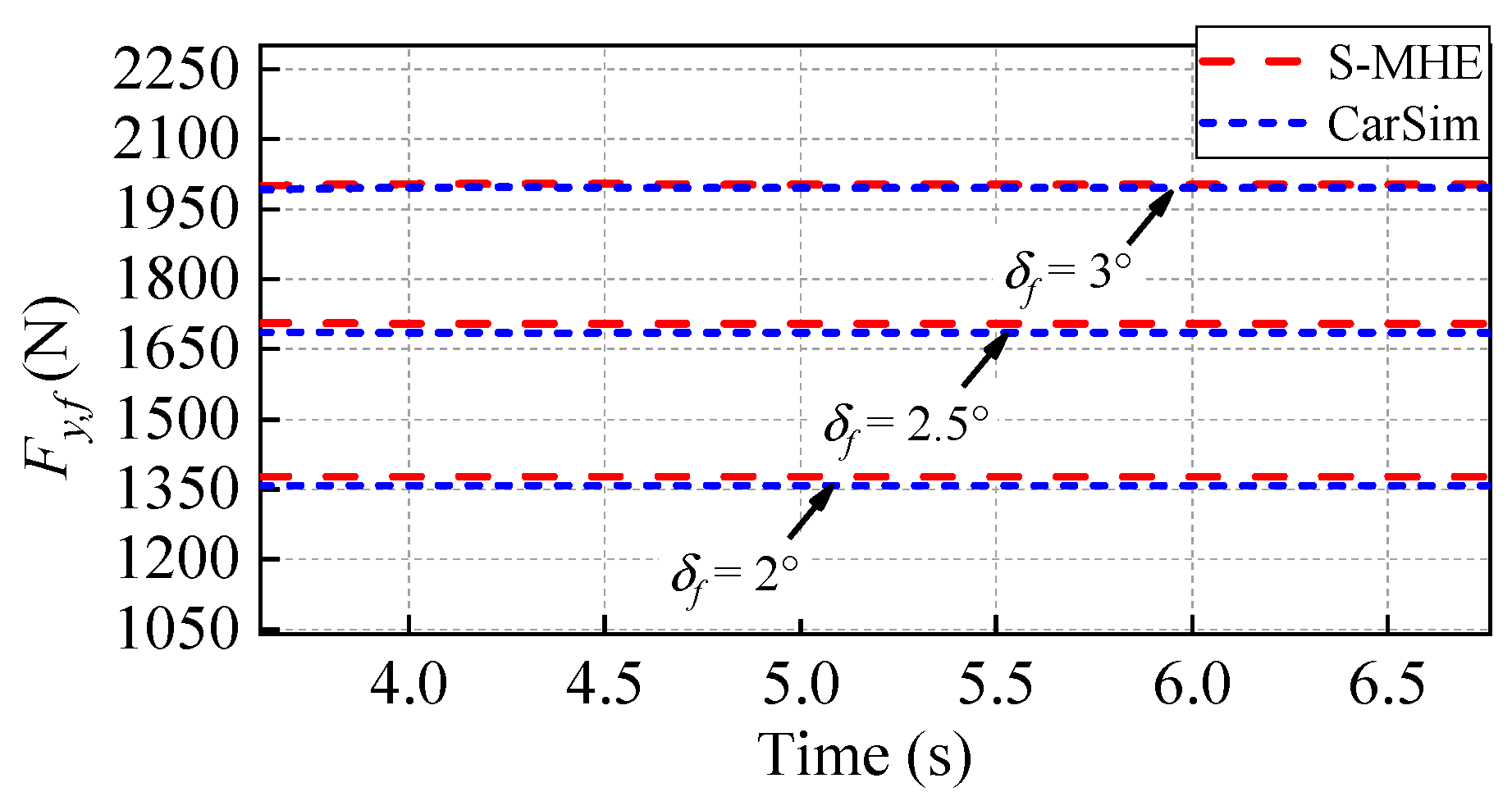
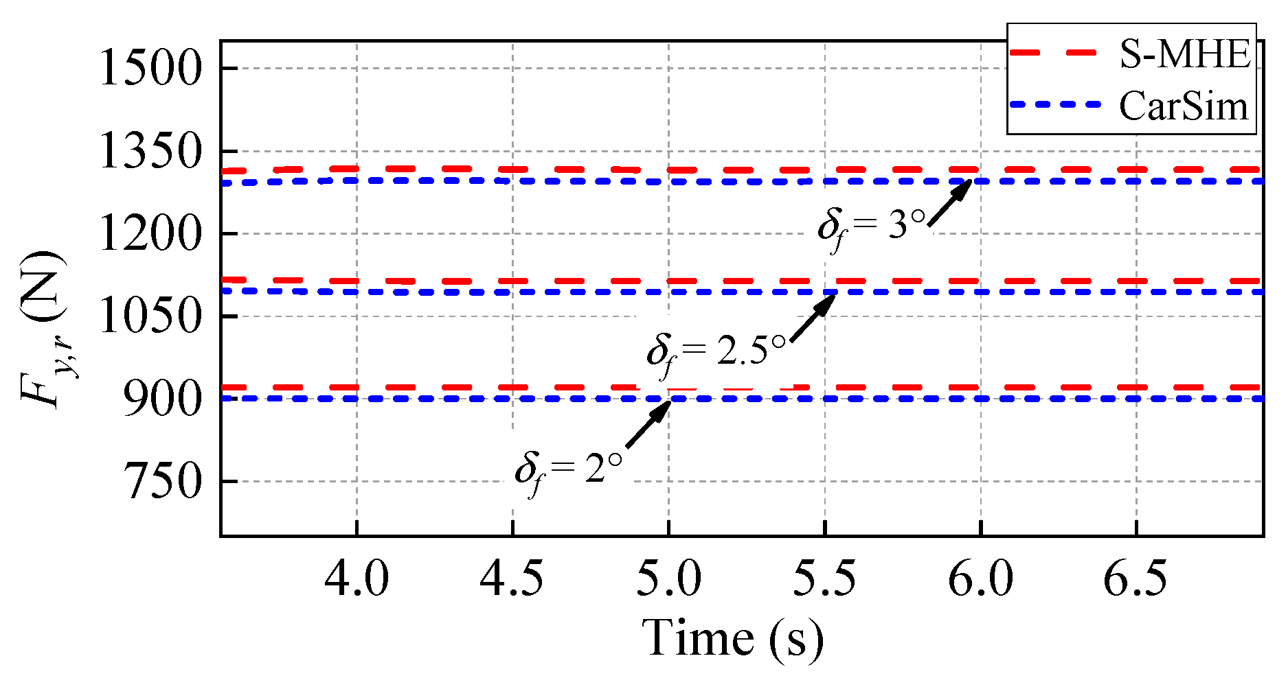
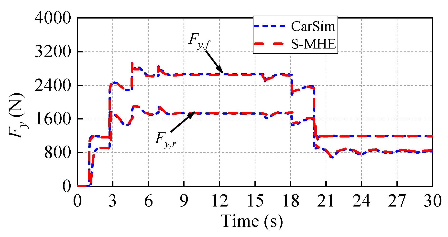
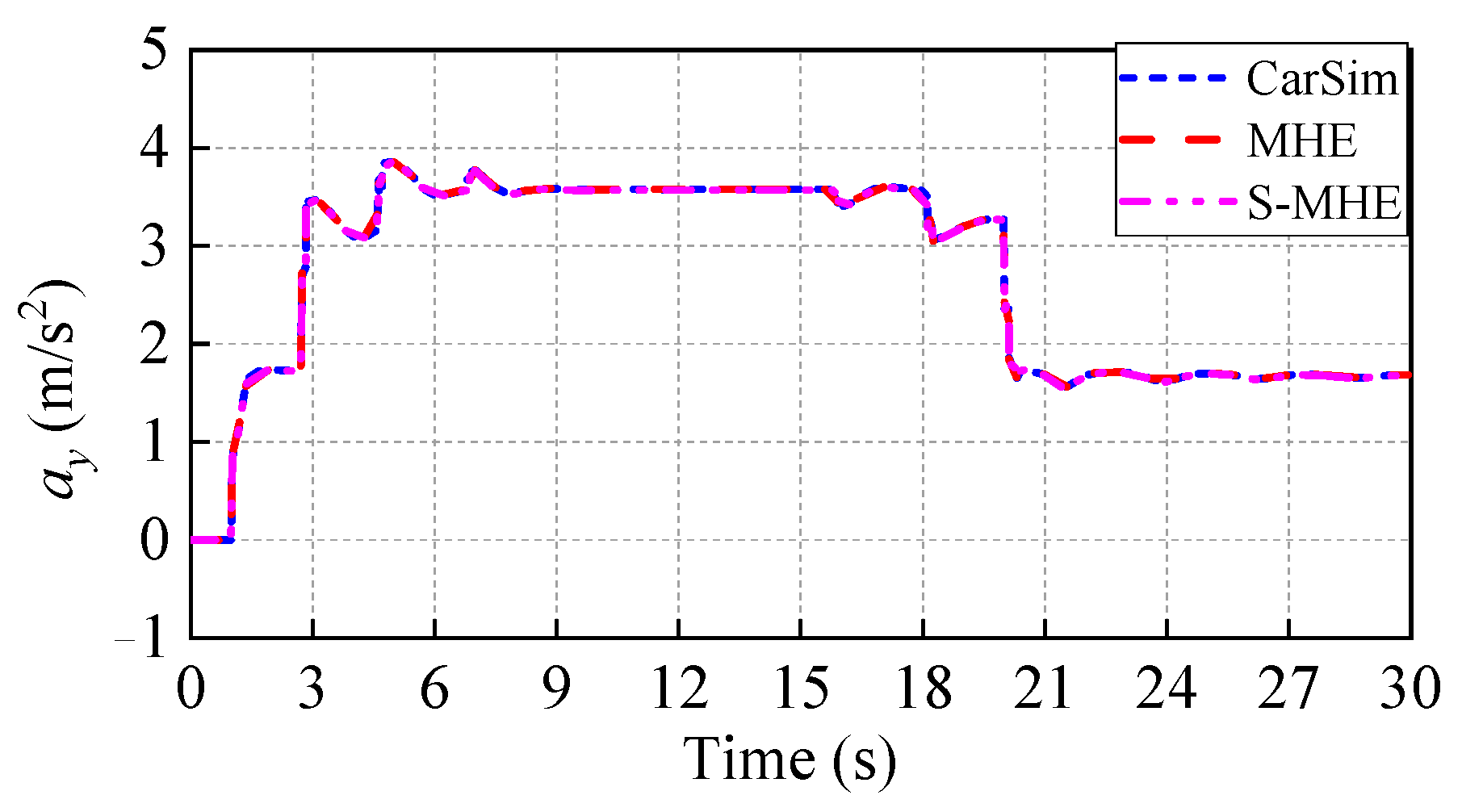
4.2. S-MHE-Based Tire Force Estimator

Due to the unique rolling optimization mechanism, MHE has high estimation accuracy and robustness. However, on the one hand, the rolling optimization mechanism brings a huge computational burden, especially for nonlinear systems. On the other hand, after the solution is obtained, the iterative calculation is required to obtain the estimation result at the current moment. This means that the variable to be estimated should be the state variable of the system (in this case, the current estimation result can be obtained by iterative calculation) or a variable that is almost unchanged within the estimation window (in this case, the solution can be directly taken as the current estimation result).

However, the estimated variable here, i.e., tire force, is not a constant value, nor is it a state variable of the system. Therefore, to realize the real-time estimation of tire force, a special MHE estimator is described in this section. In general, the length of the estimation window of MHE is adjustable. Assume that the length of the estimation window of MHE is 1; that is, only the measurements from the last moment are used, then the solution of MHE is the final estimation result. Based on the above assumptions, the special case of MHE, namely, single-step MHE, can be obtained, which is recorded as S-MHE.

For the S-MHE-based tire force estimator, the discrete estimation equation of S-MHE is as follows:

$$\mathsf{\xi }\left(k\right)=h\left({\mathsf{\varsigma }}^{\prime }\left(k\right)\right)+\mathbf{v}\left(k\right)$$

(25)

where state variables ${\mathsf{\varsigma }}^{\prime }={\left[F_{y,f},F_{y,r}\right]}^T$, $\mathbf{v}={[v_1,v_2]}^T$. The definitions of $\mathsf{\xi }$ and $h\left({\mathsf{\varsigma }}^{\prime }\right)$ can refer to Equation (19).

The cost function of the S-MHE estimator is defined as

$$\begin{array}{r}{J}_{MHE}\left(\left\{\mathbf{v}\left(k\right)\right\},{\mathsf{\varsigma }}^{\prime }\left(k\right)\right)={\Vert {\tilde{\mathsf{\xi }}}^{\prime }\left(k\right)-\mathsf{\xi }\left(k\right)\Vert }_{{\mathrm{\Gamma }}_{\mathsf{\xi }}^{\prime }}^2\\ +{\Vert {\mathsf{\varsigma }}^{\prime }\left(k\right)-{\overline{\mathsf{\varsigma }}}^{\prime }\left(k-1\right)\Vert }_{{\mathrm{\Gamma }}_{{\mathsf{\varsigma }}^{\prime }}}^2+{\Vert \mathbf{v}\left(k\right)\Vert }_{{\mathrm{\Gamma }}_{\mathbf{v}}}^2\end{array}$$

(26)

where ${\tilde{\mathsf{\xi }}}^{\prime }\left(k\right)$ is the latest measurement, ${\overline{\mathsf{\varsigma }}}^{\prime }\left(k-1\right)$ refers to the estimation result at the previous moment.

Finally, the estimation problem for S-MHE is described as

$$\begin{array}{l}\underset{\mathbf{v}\left(k\right),{\mathsf{\varsigma }}^{\prime }\left(k\right)}{\min }{J}_{MHE}\left(\mathbf{v}\left(k\right),{\mathsf{\varsigma }}^{\prime }\left(k\right)\right)\\ s.t.\hspace{1em}\mathsf{\xi }\left(k\right)=h\left({\mathsf{\varsigma }}^{\prime }\left(k\right)\right)+\mathbf{v}\left(k\right)\\ \hspace{1em}\hspace{1em}{\mathsf{\varsigma }}_{\min }^{\prime }\le {\mathsf{\varsigma }}^{\prime }\left(k\right)\le {\mathsf{\varsigma }}_{\max }^{\prime }\\ \hspace{1em}\hspace{1em}{\mathsf{\xi }}_{\min }\le \mathsf{\xi }\left(k\right)\le {\mathsf{\xi }}_{\max }\end{array}$$

(27)

where ${\mathsf{\varsigma }}_{\min }^{\prime }$ and ${\mathsf{\varsigma }}_{\max }^{\prime }$ can be taken as the maximum physical limit of the tire force on the corresponding axle.

The estimated tire force is the input of the ITM-based RFC estimator, and the design details of the ITM estimator will be introduced in the next section.

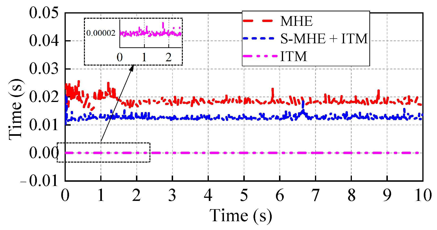
4.3. ITM-Based RFC Estimator

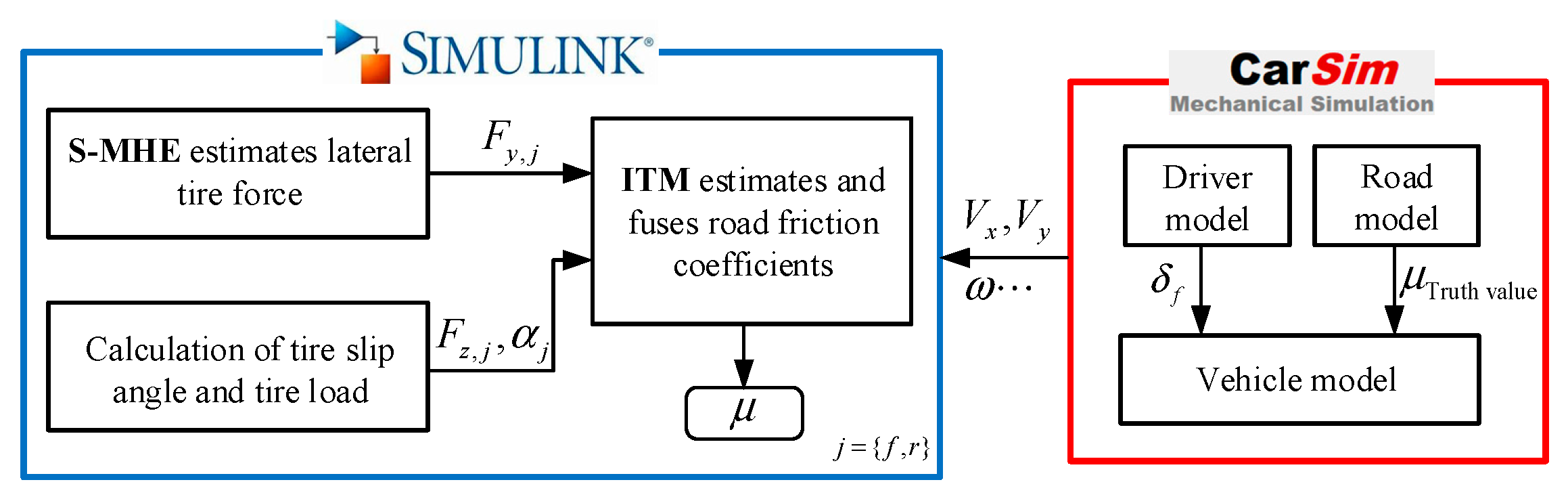
The structure of the ITM-based RFC estimator is shown in Figure 4. The input of the ITM estimator is the tire load, lateral tire force, and tire slip angle on the front and rear tires, and the output is the RFC.

Based on Equations (2)–(15), the ITM with respect to the RFC can be obtained:

$$\mu =f^{ITM}(\alpha ,\gamma ,F_y,F_z,\widehat{\mu })$$

(28)

$$f^{ITM}=\frac{F_y-S_{Vy}}{\sin [C_y\arctan \{B_y{\alpha }_y-E_y(B_y{\alpha }_y-\arctan (B_y{\alpha }_y))\}]D_y^o{\mu }_y^o}$$

(29)

$$D_y^o=F_z{\zeta }_2$$

(30)

$${\mu }_y^o=(p_{Dy1}+p_{Dy2}d{f}_z)(1-p_{Dy3}{\gamma }_y^2)$$

(31)

where $F_y$ in Equation (23) represents the tire force estimated by MHE and $\widehat{\mu }$ represents the estimated result at the previous moment, which will be used to replace $\mu$ in Equations (8) and (14). Figure 5 shows a map of the ITM with a tire load of 2500 N and a roll angle of 0 degrees.

After obtaining the RFCs on the front and rear tires, they are fused according to the following rule.

$$\mu =\frac{F_{z,f}}{F_{z,f}+F_{z,r}}{\mu }_f+\frac{F_{z,r}}{F_{z,f}+F_{z,r}}{\mu }_r$$

(32)

where ${\mu }_f$ and ${\mu }_r$ represent the RFCs on the front and rear tires. Equation (27) indicates that the tire with the larger load is given a higher weight. This is because the lateral force of a heavily loaded tire is greater, and the estimated RFC is more reliable.

5. Simulation Test

In this section, the estimation method of traditional MHE and that based on S-MHE and ITM are compared and tested based on the simulation platform of Simulink and CarSim, including the comparison test under conditions such as different steering inputs and step changes in RFC. Figure 6 shows a schematic of the simulation structure. The algorithm of the proposed friction coefficient estimation based on S-HME and ITM is implemented on the Simulink platform. The front steering input and road conditions are set on the CarSim platform. The configuration of the computing platform used in the study is as follows. Processor: Intel(R) Core(TM) i5-8500 [email protected] GHz; RAM: Kingston DDR4 2400 MHz 16.0 GB; Hard Drive: Kingston SA2000M8500G; OS: Windows 10 Education Edition.

Table 5. Parameters of CarSim and estimators.

Symbol	Description	Symbol	Description
m	1231 kg	lf	1.04 m
Iz	2031.4 kg⋅m2	lr	1.56 m
N	10	${\mathrm{\Gamma }}_{{\mathsf{\xi }}^{\prime }}$	[14,000;14,000]
${\mathrm{\Gamma }}_{\mathsf{\xi }}$	[1400;1400]	${\mathrm{\Gamma }}_{{\mathsf{\varsigma }}^{\prime }}$	[0.1;0.1]
${\mathrm{\Gamma }}_{\varsigma }$	500	${\mathrm{\Gamma }}_{\mathbf{v}}$	[1;1]
${\mathrm{\Gamma }}_v$	1	${\overline{\mathsf{\varsigma }}}^{\prime }(0)$	[0;0]
$\overline{\varsigma }(0)$	0.1

gives the main parameters of CarSim and several estimators.

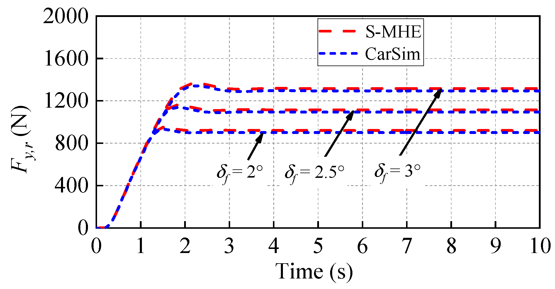
5.1. Test under Different Steering Inputs

In this test, the test vehicle was controlled with ramp front steering inputs of a maximum of 2°, 2.5°, and 3°, as shown in Figure 7. The speed of the test vehicle is 60 km/h, and the truth value of the RFC is 0.4.

Figure 8 and Figure 9 show the estimated results of the RFC output by the traditional MHE and ITM estimators, respectively. It can be seen from the results that when the maximum front steering angle input is 2°, 2.5°, and 3°, respectively, the RFCs estimated by the traditional MHE and ITM estimators are, respectively, stable at 0.431, 0.423, and 0.412 and 0.430, 0.419, and 0.408. That is, the estimated accuracy of the traditional MHE estimators is 92.25%, 94.25%, and 97.00%, respectively, and that of the ITM estimators is 92.50%, 95.25%, and 98.00%, respectively. The results show that the estimation accuracies of the two estimators are close and show a similar trend; that is, with the increase of the steering angle, the estimation accuracies gradually become higher. Evaluating the details, the accuracy of the LTM estimator is slightly higher, and the convergence speed of the traditional MHE is slightly faster.

Figure 10 and Figure 11 show the lateral forces estimated by S-MHE, which are inputs to the ITM estimator. From the partially enlarged views of the lateral forces, as shown in Figure 12 and Figure 13, it can be seen that with the increase of the front steering input, the error in the front tire lateral forces estimated by S-MHE and output by CarSim gradually decreases. In addition, the rear tire lateral force estimated by S-MHE has errors under several of the above inputs, which is mainly because the lateral force of the rear tires is small. The above results and the fusion rule of RFC (i.e., Equation (27)) explain why the RFC estimated by the ITM in Figure 9 is more accurate as the front steering angle increases.

Figure 14 and Figure 15 represent the lateral acceleration and yaw rate output by the MHE and S-MHE (output of the estimator model) and feedback by CarSim (measurements). From the results, it can be seen that the lateral acceleration and yaw rate output by the traditional MHE and S-MHE are almost identical to those feedback by CarSim. This shows that the performance of both estimators has been fully utilized.

Figure 16 presents the computation time of traditional MHE, ITM, and the total computation time of S-MHE and ITM at a front steering angle of 2.5°. The results show that the average computation time of estimation methods based on S-MHE and ITM and traditional MHE are 0.0126 s and 0.0183 s, respectively. It can also be seen that the ITM estimator consumes very little computation time. Compared with MHE, the method proposed in this study improves the real-time performance by 31.15%.

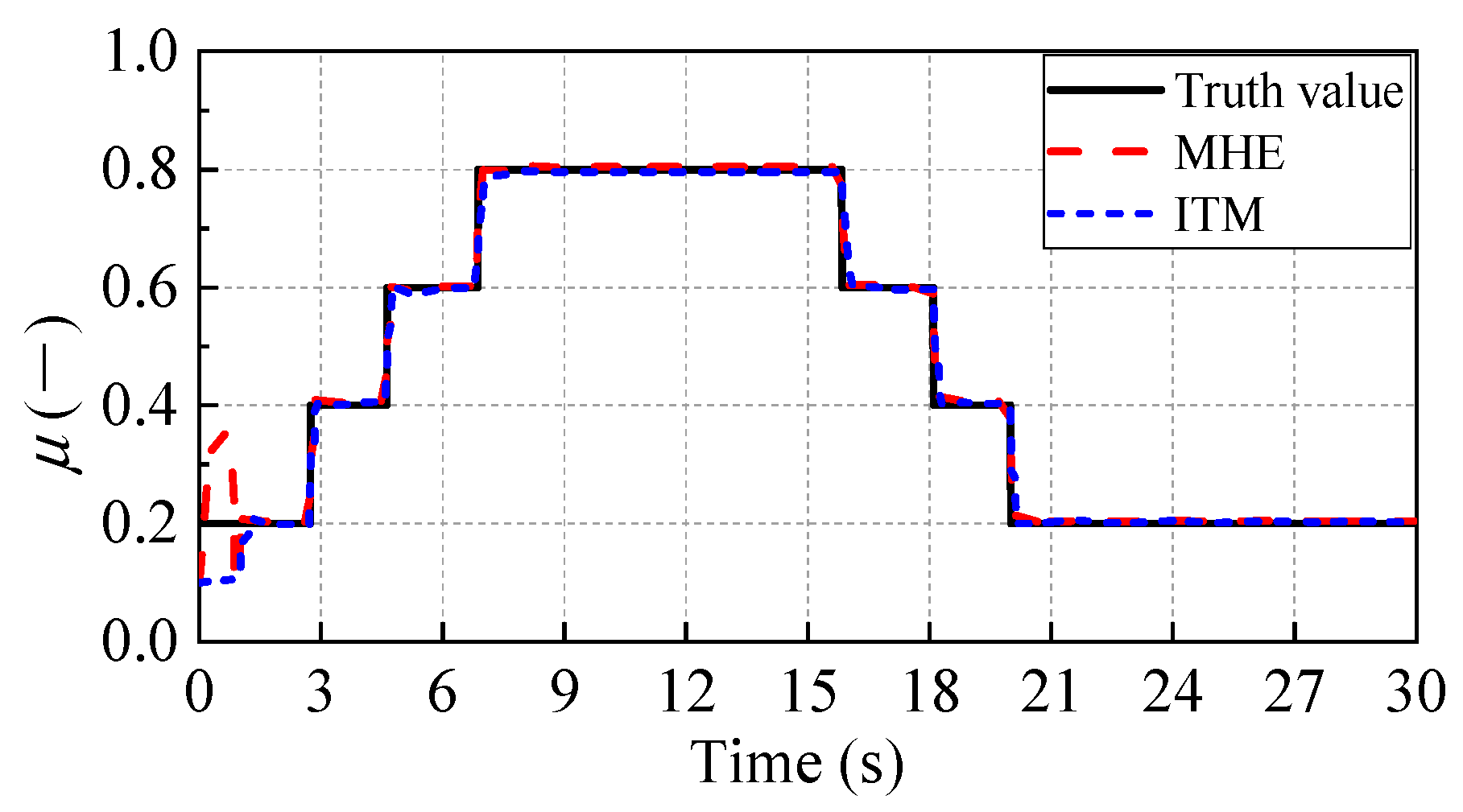
5.2. Test under the Road with Step Change of RFC

This section tests the estimation accuracy of the RFC of the traditional MHE estimator and the proposed estimator based on S-MHE and ITM when the vehicle is run on a road with a continuous step change in friction coefficient. The front steering input of the test vehicle is shown in Figure 17. The vehicle speed is 80 km/h. The road map and vehicle trajectories are shown in Figure 18.

Figure 19 shows the RFC estimated by traditional MHE and ITM. The results show that in the first second, since the steering angle of the vehicle is 0, there is a clear error in the RFC between the true value and that estimated by the MHE and ITM estimators. Subsequently, as the steering angle increases, the RFCs estimated by the MHE and ITM estimators quickly converge to the truth value, as shown in Figure 20. The results in Figure 20 also show that the convergence speed of MHE is faster, but the estimation accuracy is slightly lower than that of ITM. The average estimation error is 0.0062 and −0.0033, respectively. The above results show the same phenomena and conclusions as those in the previous section.

Figure 21 represents the lateral forces estimated by the S-MHE. It can be seen that the estimation results of the lateral force are almost consistent with the output of CarSim. Because of this, the estimation accuracy of the ITM estimator is guaranteed.

The results in Figure 22 and Figure 23 show that both the traditional MHE and S-MHE estimators perform fully in this test.

Figure 24 shows that ITM estimators require very little computation time. The average computation time of the S-MHE and ITM-based estimators and the traditional MHE estimators is 0.0125 s and 0.0181 s, respectively. Compared with the latter, the real-time performance of the former is improved by 30.94%.

6. Conclusions

To improve the estimation method of RFC based on MHE in the real-time performance, a hierarchical framework for RFC estimation is first proposed, and then a single-step MHE (S-MHE)-based tire force estimator and an inverse tire model (ITM)-based RFC estimator are designed respectively. Structurally, the proposed hierarchical framework decouples vehicle dynamics and tire dynamics and decomposes the problem of RFC estimation based on the complex nonlinear system of vehicle-tire dynamics into two relatively simple estimation problems, namely, the estimation problem of tire force based on the vehicle model and the estimation problem of RFC based on inverse tire model. In the algorithm, on the one hand, the designed S-MHE estimator realizes the estimation of variables that are not system states and reduces the calculation burden. On the other hand, the designed ITM estimator only needs forward calculation to obtain the estimation result, which requires little computing resources.

Simulation tests show that, under the condition of an RFC of 0.4 and a vehicle speed of 60 km/h, the proposed hierarchical estimation method can achieve an estimation accuracy of more than 92.50% when the steering angle is greater than 2°, which is slightly higher than that of the traditional MHE. Moreover, the calculation speed is increased by 31.15%. On the road with step change of RFC, when the vehicle speed is 80 km/h and the steering angle is 3°, the average estimation error of the proposed estimation method is 0.0033, which is lower than 0.0062 of the traditional MHE, and the real-time performance is improved by 30.94%. The results demonstrate that the proposed method can significantly improve real-time performance while maintaining estimation accuracy.

References

1. Chang, F.R.; Huang, H.L.; Schwebel, D.C.; Chan, A.H.; Hu, G.Q. Global road traffic injury statistics: Challenges, mechanisms and solutions. Chin. J. Traumatol. 2020, 23, 216–218. [Google Scholar] [CrossRef] [PubMed]
2. Pisano, P.A.; Goodwin, L.C.; Rossetti, M.A. US highway crashes in adverse road weather conditions. In Proceedings of the 24th Conference on International Interactive Information and Processing Systems for Meteorology, Oceanography and Hydrology, New Orleans, LA, USA, 20 January 2008. [Google Scholar]
3. Brodsky, H.; Hakkert, A.S. Risk of a road accident in rainy weather. Accid. Anal. Prev. 1988, 20, 161–176. [Google Scholar] [CrossRef] [PubMed]
4. Khaleghian, S.; Emami, A.; Taheri, S. A technical survey on tire-road friction estimation. Friction 2017, 5, 123–146. [Google Scholar] [CrossRef] [Green Version]
5. Jumaa, B.A.; Abdulhassan, A.M.; Abdulhassan, A.M. Advanced driver assistance system (ADAS): A review of systems and technologies. Int. J. Adv. Res. Comput. Eng. Technol. (IJARCET) 2019, 8, 231–234. [Google Scholar]
6. Li, S.; Wang, G.; Chen, G.; Chen, H.; Zhang, B. Tire State Stiffness Prediction for Improving Path Tracking Control during Emergency Collision Avoidance. IEEE Access 2019, 7, 179658–179669. [Google Scholar] [CrossRef]
7. Wang, G.; Liu, L.; Meng, Y.; Gu, Q.; Bai, G. Integrated Path Tracking Control of Steering and Differential Braking Based on Tire Force Distribution. Int. J. Control. Autom. Syst. 2022, 20, 536–550. [Google Scholar] [CrossRef]
8. Acosta, M.; Kanarachos, S.; Blundell, M. Road Friction Virtual Sensing: A Review of Estimation Techniques with Emphasis on Low Excitation Approaches. Appl. Sci. 2017, 7, 1230. [Google Scholar] [CrossRef] [Green Version]
9. Wang, G.; Liu, L.; Meng, Y.; Wang, S.; Gu, Q.; Bai, G. MHE-Based Friction Coefficient Estimation and Compensation Method for Path Tracking Control. In Proceedings of the 2022 IEEE 25th International Conference on Intelligent Transportation Systems (ITSC), Macau, China, 8–12 October 2022; pp. 146–152. [Google Scholar]
10. Wang, H.; Liu, B. Path Planning and Path Tracking for Collision Avoidance of Autonomous Ground Vehicles. IEEE Syst. J. 2021, 16, 3658–3667. [Google Scholar] [CrossRef]
11. Wang, Y.; Lv, C.; Yan, Y.; Peng, P.; Wang, F.; Xu, L.; Yin, G. An Integrated Scheme for Coefficient Estimation of Tire–Road Friction With Mass Parameter Mismatch Under Complex Driving Scenarios. IEEE Trans. Ind. Electron. 2021, 69, 13337–13347. [Google Scholar] [CrossRef]
12. Wang, Y.; Hu, J.; Wang, F.; Dong, H.; Yan, Y.; Ren, Y.; Zhou, C.; Yin, G. Tire Road Friction Coefficient Estimation: Review and Research Perspectives. Chin. J. Mech. Eng. 2022, 35, 6. [Google Scholar] [CrossRef]
13. Gustafsson, F. Slip-based tire-road friction estimation. Automatica 1997, 33, 1087–1099. [Google Scholar] [CrossRef]
14. Lee, C.; Hedrick, K.; Yi, K. Real-Time Slip-Based Estimation of Maximum Tire–Road Friction Coefficient. IEEE/ASME Trans. Mechatron. 2004, 9, 454–458. [Google Scholar] [CrossRef]
15. Rajamani, R.; Phanomchoeng, G.; Piyabongkarn, D.; Lew, J.Y. Algorithms for Real-Time Estimation of Individual Wheel Tire-Road Friction Coefficients. IEEE/ASME Trans. Mechatron. 2011, 17, 1183–1195. [Google Scholar] [CrossRef]
16. Guan, H.; Wang, B.; Lu, P.; Xu, L. Identification of maximum road friction coefficient and optimal slip ratio based on road type recognition. Chin. J. Mech. Eng. 2014, 27, 1018–1026. [Google Scholar] [CrossRef]
17. Enisz, K.; Szalay, I.; Kohlrusz, G.; Fodor, D. Tyre–road friction coefficient estimation based on the discrete-time extended Kalman filter. Proc. Inst. Mech. Eng. Part D J. Automob. Eng. 2015, 229, 1158–1168. [Google Scholar] [CrossRef]
18. Ray, L.R. Nonlinear tire force estimation and road friction identification: Simulation and experiments. Automatica 1997, 33, 1819–1833. [Google Scholar] [CrossRef]
19. Andersson, M.; Bruzelius, F.; Casselgren, J.; Hjort, M.; Löfving, S.; Olsson, G.; Rönnberg, J.; Sjödahl, M.; Solyom, S.; Svendenius, J.; et al. Road Friction Estimation Part II; Intelligent Vehicle Safety Systems (IVSS) Project Report; IVSS/Swedish Road Administration: Borlange, Sweden, 2010. [Google Scholar]
20. Muller, S.; Uchanski, M.; Hedrick, K. Estimation of the Maximum Tire-Road Friction Coefficient. J. Dyn. Syst. Meas. Control. 2003, 125, 607–617. [Google Scholar] [CrossRef]
21. Andrieux, A.; Vandanjon, P.O.; Lengellé, R.; Chabanon, C. New results on the relation between tyre–road longitudinal stiffness and maximum available grip for motor car. Veh. Syst. Dyn. 2010, 48, 1511–1533. [Google Scholar] [CrossRef]
22. Ma, B.; Lv, C.; Liu, Y.; Zheng, M.; Yang, Y.; Ji, X. Estimation of Road Adhesion Coefficient Based on Tire Aligning Torque Distribution. J. Dyn. Syst. Meas. Control. 2018, 140, 051010. [Google Scholar] [CrossRef]
23. Hsu YH, J.; Laws, S.M.; Gerdes, J.C. Estimation of tire slip angle and friction limits using steering torque. IEEE Trans. Control. Syst. Technol. 2009, 18, 896–907. [Google Scholar] [CrossRef]
24. Gao, X.; Yu, Z.; Neubeck, J.; Wiedemann, J. Sideslip angle estimation based on input–output linearisation with tire–road friction adaptation. Veh. Syst. Dyn. 2010, 48, 217–234. [Google Scholar] [CrossRef]
25. Wang, F.; Wang, S.; Wang, S.; Li, S.; Zhang, B.; Cui, G. Collision Avoidance Control by steering based on Moving Horizon Estimation Control. In Proceedings of the 2020 4th CAA International Conference on Vehicular Control and Intelligence (CVCI), Hangzhou, China, 8–20 December 2020; pp. 147–152. [Google Scholar]
26. Luque, P.; Mántaras, D.A.; Fidalgo, E.; Álvarez, J.; Riva, P.; Girón, P.; Compadre, D.; Ferran, J. Tyre–road grip coefficient assessment—Part II: Online estimation using instrumented vehicle, extended Kalman filter, and neural network. Veh. Syst. Dyn. 2013, 51, 1872–1893. [Google Scholar] [CrossRef]
27. Liu, Y.H.; Li, T.; Yang, Y.Y.; Ji, X.W.; Wu, J. Estimation of tire-road friction coefficient based on combined APF-IEKF and iteration algorithm. Mech. Syst. Signal Process. 2017, 88, 25–35. [Google Scholar] [CrossRef]
28. Haseltine, E.L.; Rawlings, J.B. Critical evaluation of extended Kalman filtering and moving-horizon estimation. Ind. Eng. Chem. Res. 2005, 44, 2451–2460. [Google Scholar] [CrossRef]
29. Zhao, L.; Liu, Z.; Chen, H. The estimation of vehicle speed and tire-road adhesion coefficient using moving horizon strategy. Automot. Eng. 2009, 31, 520–525. [Google Scholar]
30. Rawlings, J.B.; Bakshi, B.R. Particle filtering and moving horizon estimation. Comput. Chem. Eng. 2006, 30, 1529–1541. [Google Scholar] [CrossRef]
31. Koskinen, S. Sensor Data Fusion Based Estimation of Tyre-Road Friction to Enhance Collision Avoidance; Tampere University of Technology: Tampere, Suomi, 2010. [Google Scholar]
32. Zanon, M.; Frasch, J.V.; Diehl, M. Nonlinear moving horizon estimation for combined state and friction coefficient estimation in autonomous driving. In Proceedings of the 2013 European Control Conference (ECC), Zurich, Switzerland, 17–19 July 2013; pp. 4130–4135. [Google Scholar]
33. Pacejka, H. Tire and Vehicle Dynamics, 3rd ed.; Elsevier Science: Burlington, MA, USA, 2012. [Google Scholar]
Figure 1. The overall structure of the proposed hierarchical estimation method.
Electronics 12 00525 g001
Figure 2. Vehicle model.
Electronics 12 00525 g002
Figure 3. MHE schematic diagram.
Electronics 12 00525 g003
Figure 4. Schematic diagram of the ITM estimator.
Electronics 12 00525 g004
Figure 5. Map of the inverse tire model.
Electronics 12 00525 g005
Figure 6. Simulation structure.
Electronics 12 00525 g006
Figure 7. Ramp input of steering angle.
Electronics 12 00525 g007
Figure 8. RFC estimated by traditional MHE.
Electronics 12 00525 g008
Figure 9. RFC estimated by ITM.
Electronics 12 00525 g009
Figure 10. Lateral tire force at front tire estimated by S-MHE.
Electronics 12 00525 g010
Figure 11. Lateral tire force at rear tire estimated by S-MHE.
Electronics 12 00525 g011
Figure 12. A partially enlarged view of front lateral tire force.
Electronics 12 00525 g012
Figure 13. A partially enlarged view of rear lateral tire force.
Electronics 12 00525 g013
Figure 14. Lateral acceleration.
Electronics 12 00525 g014
Figure 15. Yaw rate.
Electronics 12 00525 g015
Figure 16. The computation time.
Electronics 12 00525 g016
Figure 17. Step input of steering angle.
Electronics 12 00525 g017
Figure 18. Road map and vehicle trajectory.
Electronics 12 00525 g018
Figure 19. RFC estimated by traditional MHE and ITM.
Electronics 12 00525 g019
Figure 20. A partially enlarged view of the estimation RFC.
Electronics 12 00525 g020
Figure 21. Lateral tire forces estimated by S-MHE.
Electronics 12 00525 g021
Figure 22. Lateral acceleration.
Electronics 12 00525 g022
Figure 23. Yaw rate.
Electronics 12 00525 g023
Figure 24. The computation time.
Electronics 12 00525 g024