Sawtooth V-Trough Cavity for Low-Concentration Photovoltaic Systems Based on Small-Scale Linear Fresnel Reflectors: Optimal Design, Verification, and Construction

Abstract

Ensuring the uniformity of solar irradiance distribution on photovoltaic cells is a major challenge in low-concentrating photovoltaic systems based on a small-scale linear Fresnel reflector. A novel sawtooth V-cavity design method based on an optimization algorithm to achieve uniform irradiance distribution on photovoltaic cells is presented. The reliability of the design was verified using the Monte Carlo ray-tracing method and a laser experiment. A prototype was built using 3D printing technology with a biodegradable green polymer material known as polylactic acid. The new cavity was compared to the standard V-trough cavity, keeping the cavity aperture, reflective surface area, and photovoltaic cell width constant. In addition, the focal height, number of mirrors, mirror width, and mirror spacing were also kept constant; so, the cost of the two configurations was the same from the point of view of the primary reflector system. The new design ensured the uniform distribution of solar irradiation and significantly reduced the height of the cavity. The significant decrease in the height of the proposed cavity has the following advantages: (i) a decrease in the dimensions of the fixed structure of the small-scale linear Fresnel reflector, thus reducing its cost, (ii) a significant decrease in the surface area exposed to wind loads, thus reducing the cost of the fixed structure and secondary system structures, (iii) a reduction in the difficulty of the manufacture, maintenance, and transportation of the cavity’s reflecting walls, and (iv) an increase in the cooling surface area, which increases the electrical efficiency of the photovoltaic cells.

1. Introduction

Solar energy is one of the renewable energy sources that will replace fossil fuels and has received increasing attention due to its properties. The energy produced is clean, free, and unlimited. Moreover, solar photovoltaic ($PV$) technology is one of the systems that harnesses solar energy and has the potential to generate electricity worldwide.

Concentrated and non-concentrated solar power are two applications of solar $PV$ energy that can produce electricity. A concentrated photovoltaic ($CPV$) system uses optical devices to concentrate the incident solar irradiance onto a smaller area, thereby increasing the solar energy flux reaching the $PV$ cells. $CPV$ technology can be classified into three categories: low-concentration photovoltaics ($LCPV$), medium-concentration photovoltaics ($MCPV$), and high-concentration photovoltaics ($HCPV$). A concentration from 2 suns to 10 suns is used in $LCPV$, from 10 suns to 100 suns in $MCPV$ and from 100 suns to 1000 suns in $HCPV$ [1].

Some of the characteristics of concentrated and non-concentrated systems are explained below:

(i)

The use of non-concentrated solar energy has significantly increased its presence in the electricity sector, mainly due to the lower costs. Based on a recent report from the International Renewable Energy Agency ($IRENA$) [2], the levelized cost of energy ($LCOE$) from non-concentrated photovoltaic ($PV$) systems is expected to decrease by $0.05$ (USD/kWh) by 2050. The lower cost of $PV$ modules is one of the main reasons for this decrease [3]. In this regard, the International Renewable Energy Agency ($IRENA$) presented a report in 2017 predicting a $60\%$ drop in the cost of $PV$ modules over the following 10 years [4]. The spot price of a $PV$ module is currently USD 0.266/$Wp$ [5]. Concentrated $PV$ systems replace the large surface area of photovoltaic cells used in non-concentrated photovoltaic systems with cheaper optical materials (e.g., lenses or mirrors), which thus reduces the cost of these systems.

(ii)

As with any other technology, non-concentrated solar power ages and degrades over time. Manufacturers of silicon-based $PV$ modules estimate their lifetime to be about 20–25 years. After that, the $PV$ module components need to be dismantled and properly recycled. In 2016, the International Renewable Energy Agency ($IRENA$) and the International Energy Agency Photovoltaic Power Systems ($IEA\text{-}PVPS$) [6] presented the first global projections for future $PV$ module waste volumes up to 2050. Annual $PV$ module waste accounted for 250,000 tons in 2016. However, the contribution of global waste from $PV$ modules is expected to considerably increase in the coming years. Waste generation from solar $PV$ modules is estimated to reach $1.7$ million tons by 2030 and will continue to increase to around 60 million tons by 2050 [6]. The significant decrease in the large surface area of $PV$ cells used in non-concentrated systems and thus in the resulting waste is one of the main advantages of concentrated $PV$ systems.

(iii)

The conversion efficiency of $PV$ cells used in non-concentrated systems is relatively low, typically around 10–20% for commercially available silicon cells [2]. This figure can be up to $39\%$ for more sophisticated multijunction cells used in $CPV$ systems [2]. Hasan et al. [7] demonstrated that a $CPV$ with p-Si solar cells improved the Pmax by $62.5\%$ more than a non-concentrated p-Si solar panel.

(iv)

Concentrated systems only use the direct component of solar irradiance and therefore require an accurate solar tracking system [8]. The cost of these systems is not very high when using a small-scale linear Fresnel reflector [9].

(v)

The temperature of a cell increases with the increase in solar irradiance concentration, thus leading to a loss in solar cell efficiency. For this reason, concentrated $PV$ systems are equipped with a cooling system. In addition to reducing the cell temperature, cooling systems can also be used to heat water in household applications if a low-concentration photovoltaic system is used. This dual use increases the energy efficiency of the system. Kandilli [10] evaluated the overall efficiency of a $CPV$ system at over $65.1\%$.

(vi)

The available surface area on building roofs is key for the implementation of $PV$ systems in buildings [11]. Low-concentration $PV$ systems require $60\%$ less surface area to produce the same thermal and electrical performance compared to separate $PV$ and thermal modules [12].

(vii)

The installation cost of an $LCPV$ system can be more than double ($2.3$ times) the cost of a non-concentrated $PV$ system [13]. However, under suitable conditions of high direct irradiation (>2.5 (MWh/m² year)) and at utility scale, $CPV$ technologies have proven to be competitive with non-concentrated photovoltaic systems [14].

Studies have shown that solar concentrators are suitable for $LCPV$ applications [1]. Therefore, $LCPV$ systems can be based on different solar concentrators: parabolic dishes [15], parabolic concentrators [16], Fresnel lenses [17], and small-scale linear Fresnel reflectors ($SSLFRs$) [18,19].

Low-concentration photovoltaic systems based on small-scale linear Fresnel reflectors are the subject of this study. This solar concentrator uses stretched rows of mirrors to focus direct solar irradiance incident on $PV$ cells running longitudinally above the rows of mirrors over a common focal line across the mirrors [18]. The cavities commonly used in these systems are a standard V-trough cavity [20] and a standard compound parabolic cavity [21]. The standard compound parabolic cavity is difficult to manufacture [22] and therefore comes at a high cost. The standard V-trough cavity has the advantage of being easy to manufacture and low in cost [23]. Ustaoglu et al. [23] presented a comparative study between the standard V-trough cavity and the standard compound parabolic cavity with a constant concentration ratio and the $PV$ cell width. The maximum acceptance angle in the case of the standard V-trough cavity was $32.25\%$ higher. This result was beneficial when using this cavity in an $SSLFR$, as it allowed the use of wider mirrors. The standard V-trough cavity is analyzed to determine whether the cost of $LCPV$ systems may be lowered. A standard V-trough cavity consists of two flat reflectors inclined at an angle ($\tau$) to the aperture of the cavity. The critical parameters governing the ray acceptance in this cavity are the flux concentration ratio ($C_{opt}$), the trough wall angle ($\tau$), and the height of the cavity (H).

Several authors have studied these types of cavities. Otanicar et al. [24] presented the design of a standard V-trough cavity with a $PV$ cell width of 20 mm, an aperture of $229.60$ mm, and a cavity height of $87.93$ mm. Al-Shohani et al. [25] presented different standard V-trough cavity designs with varying geometric parameters, geometric concentration ratios, and reflective materials. A standard V-cavity was used in the design of a daylighting system based on optical fiber bundles and a small-scale linear Fresnel reflector [26]. Concentrated photovoltaic systems based on a small-scale Fresnel reflector have also used the standard V-trough cavity [27]. All these studies used a standard V-trough cavity. This paper presents another view of the use of this cavity.

As has already been seen, one of the drawbacks hindering the expansion of $LCPV$ systems is their cost in comparison to non-concentrated $PV$ systems. This means, a lower solar concentrator cost would facilitate the use of these systems. In the case of $SSLFRs$, the parameter that most influences the cost has been proven to be the number of mirrors [28]. Fewer mirrors brings a lower cost. Decreasing the number of mirrors requires increasing the width of the mirrors and thus the aperture of the cavity. This requirement implies that the standard V-trough cavity would need a greater height. Increasing the height of the cavity increases the overall cost of the $SSLFR$. Therefore, there is a need for a new cavity design.

The homogeneous distribution of solar irradiance on the $PV$ cells is the most important design condition in an $LCPV$ system. If this condition is not met, the fill factor and overall electrical efficiency decrease [29], a situation that may even damage the cells [30]. The standard V-trough cavity can fulfill this design condition if the parameters are properly calculated, which is a significant advantage favoring its use [31]. Therefore, this condition was taken into account when designing the new cavity.

The objectives of this study are as follows:

(i)

The optimal design of a sawtooth V-trough cavity, which ensures uniform illumination of the photovoltaic cells;

(ii)

The verification of the designed sawtooth V-cavity to confirm that the derived equations are correct;

(iii)

The manufacture of the designed sawtooth V-cavity, in order to identify any manufacturing difficulties;

(iv)

Experimental tests to show that the manufactured sawtooth cavity meets the specifications.

The specific contributions of this study can be summarized in the following proposals:

(i)

A methodology for designing a new sawtooth V-cavity;

(ii)

A significant reduction in the cavity height of the proposed sawtooth V-trough cavity;

(iii)

After (ii), a considerable reduction in the cost of manufacturing an $SSLFR$;

(iv)

A comparison between the proposed sawtooth V-cavity and the standard V-cavity, considering that both cavities have the same cavity opening and the same $PV$ cell width;

(v)

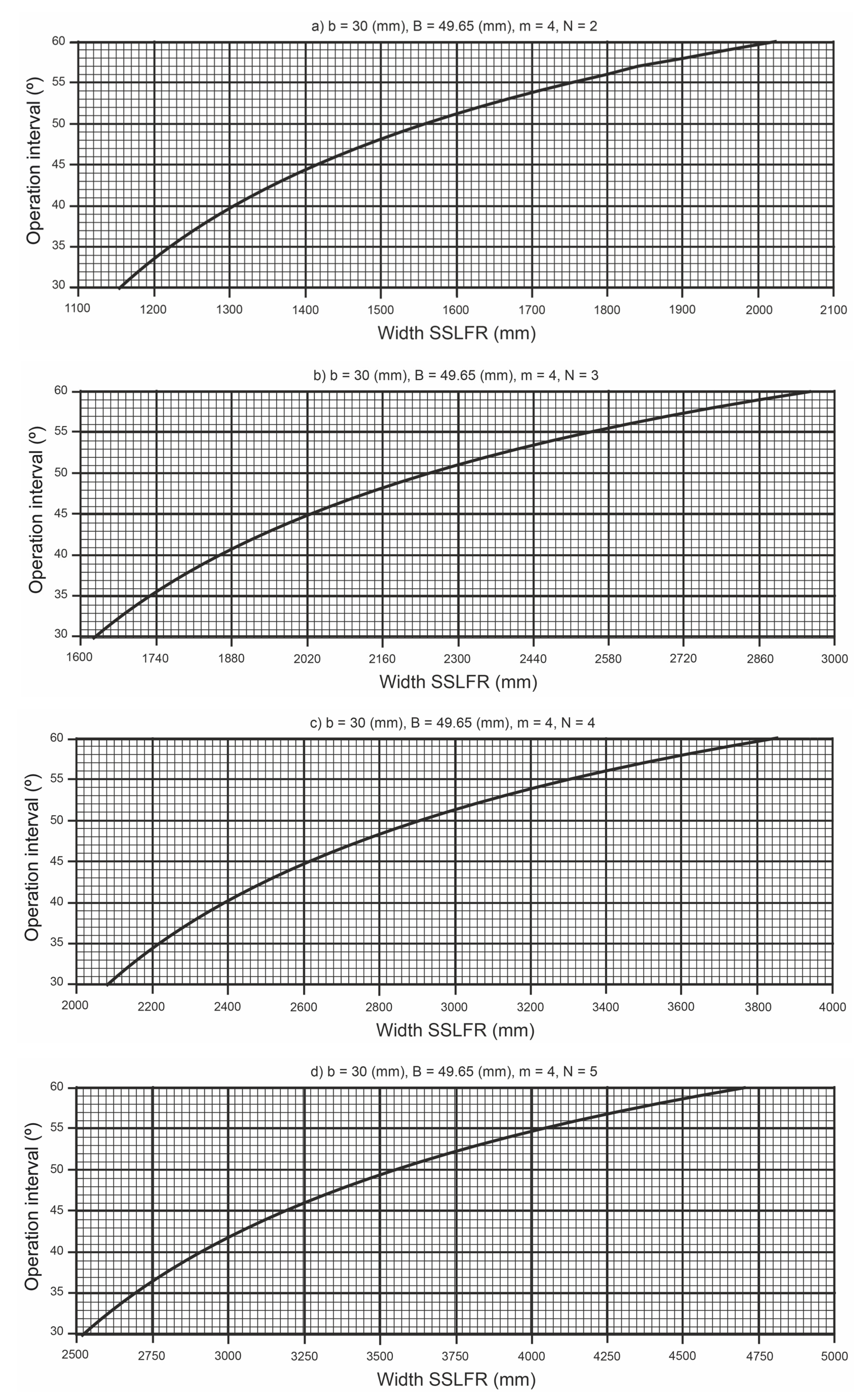
The presentation of a novel graphical system to design the primary reflector system for the $SSLFR$.

The paper is organized as follows: The main parameters of an $SSLFR$ used in a low-concentration $PV$ system are reviewed in Section 2. Section 3 explains the design idea for the proposed sawtooth V-trough cavity, the optimization algorithm, the verification thereof using a Monte Carlo simulation, the manufacture of the cavity, and a laser beam experiment. Numerical simulations, verifications, and a comparative analysis are described in Section 4, and finally, Section 5 summarizes the main contributions and conclusions of the paper.

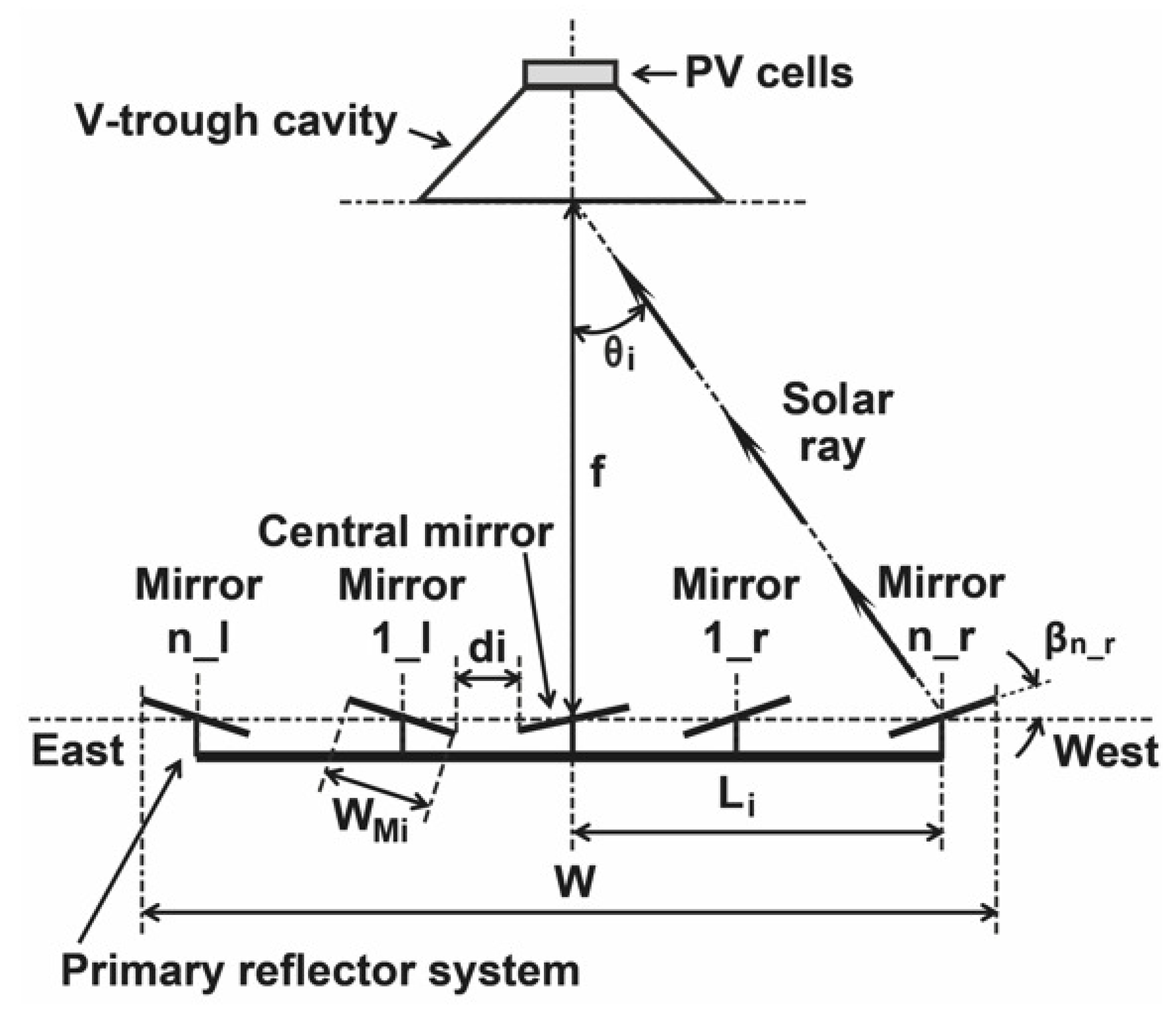
2. Overview of an SSLFR

The proposed $LCPV$ system is based on an $SSLFR$. The characteristics of this $LCPV$ system are described in [18]. The most important features thereof are:

(i)

The primary reflector system (see Figure 1).

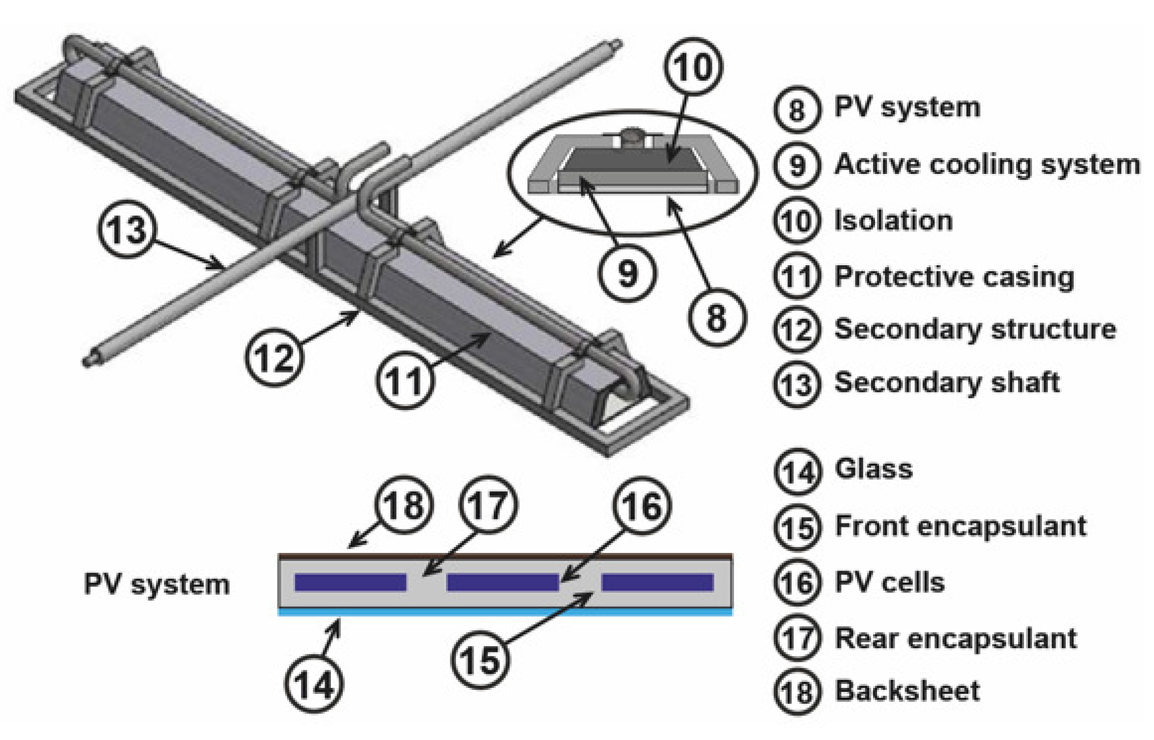
This system is installed on a mobile structure and includes parallel mirror rows and a tracking system [32]. The primary system parameters of interest for this study are shown in Figure 2 and are defined as follows: $W_{Mi}$ is the width of the i-th mirror, f is the height to the receiver, $d_i$ is the separation between two consecutive mirrors, $L_i$ is the position of each mirror with respect to the central mirror (in central mirror $i=0$ and $L_0=0$), N is the number of mirrors on each side of the central mirror (the same number of mirrors on each side is assumed; therefore, the total number of mirrors of the $SSLFR$ is: $2N+1$), ${\beta }_i$ is the angle that mirror i forms with the horizontal line, and ${\theta }_i$ is the angle between the vertical line at the focal point and the line connecting the center point of each mirror to the focal point. For each side of the $SSLFR$, ${\theta }_i$ can be determined as follows [33]:

$${\theta }_i=arctan\frac{L_i}{f};1\le i\le N.$$

(1)

The maximum ${\theta }_i$ on each side (that is, ${\theta }_{N_r}={\theta }_{N_l}$) is the acceptance angle of the V-trough cavity:

$${\theta }_c={\theta }_N.$$

(2)

The rows of mirrors synchronously follow the sun’s daily movement. The movement of the mirrors is defined by their axis of rotation, the north–south axis, and by the transverse angle ${\theta }_t$ [33]:

$${\theta }_t=arctan\left(\frac{sin{\gamma }_S}{tan{\alpha }_S}\right),$$

(3)

where ${\alpha }_S$ is the solar altitude (°), and ${\gamma }_S$ is the solar azimuth (°), both of which depend on the declination $\delta$, latitude $\lambda$, and hour angle $\omega$ [34].

The sun ray is considered to be incident on the midpoint of the mirror i and reflected towards the focal point of the cavity; therefore, the following is fulfilled [33]:

$${\beta }_i=\frac{-{\theta }_t\pm {\theta }_i}{2};1\le i\le N,$$

(4)

where ± means: − for mirrors on the left side and + otherwise. By convention, ${\beta }_i>0$ when measured counterclockwise above the horizontal line.

Another parameter needed for the uniform distribution of flux on the $PV$ cells is what is known as $W_{fi}$, which is defined as the width of the $PV$ cells illuminated by the i-th mirror [33]:

$$W_{fi}=W_{Mi}·\left[cos{\beta }_i\pm sin{\beta }_{i}tan{\theta }_i\right];1\le i\le N.$$

(5)

Taking into account that ${\theta }_i$ and ${\beta }_i$ depend on $W_{Mi}$, $d_i$, N, and f (where the value of f is usually $1.5$ m [18,35,36]), these parameters must be optimized ($W_{Mi}$, $d_i$, and N) to achieve a uniform flux distribution in the $PV$ cells [18]. The width of the $SSLFR$ (W) can be calculated as [33]:

$$W=2·L_n+W_{Mi}.$$

(6)

(ii)

The secondary system (see Figure 3).

This system is installed on a fixed structure and includes the V-trough cavity, the $PV$ system, the active cooling system, the secondary structure, the isolation material, the protective casing, and the shaft. The $PV$ cells in the $PV$ system are interconnected and encapsulated. Since a large part of the solar irradiance captured by the $PV$ cells is transformed into heat, a cooling system is available to increase the system efficiency. The standard V-trough cavity is symmetrical with respect to the central mirror in the primary system. The standard V-trough cavity parameters of interest for this study are shown in Figure 4 and are defined as follows: $W_{PV}$ is the width of the $PV$ cells, b is the absorber width of the V-trough cavity ($b=W_{PV}$), B is the aperture of the V-trough cavity, H is the height of the V-trough cavity, and $\tau$ is the trough wall angle.

For this paper, the standard V-trough cavity has been replaced with a new sawtooth V-trough cavity that was optimized by utilizing the Mathematica™ Computer Algebra System.

3. Methodology

If the design is not correct, a fraction of the incident solar irradiance will reach the base of the V-trough cavity either directly or through further reflections, and the remaining fraction will eventually escape to the outside of the V-trough cavity after further reflections, when a beam of solar irradiance is incident on the V-trough aperture at the angle provided by one of the mirrors in the primary system. Preventing this fraction of the incident solar irradiance from escaping to the outside of the V-trough cavity is the aim of this research. Another, equally important objective of this design is to achieve the uniform illumination of the photovoltaic cells in order to avoid the detrimental effects of nonuniform illumination.

3.1. The Main Elements of a Concentrator

Shoeibi et al. [37] states that the most common definition of the concentration ratio, area, or geometric concentration ratio is:

$$C_a=\frac{\mathrm{aperture}\mathrm{area}}{\mathrm{absorber}\mathrm{area}}=\frac{A_a}{A_{abs}}.$$

(7)

This ratio has an upper limit. For a two-dimensional (linear) concentrator, such as our V-trough design, and for a given acceptance half angle ${\theta }_c$, this limit is:

$$C_{ideal}^{2D}={sin}^{-1}{\theta }_c.$$

(8)

Compound parabolic concentrators ($CPC$) are known to actually reach this limit [38]. There are other indices in the literature that measure the goodness of a concentrator. The following notation (also used, for instance, in [25,39,40]) is used for this paper:

$$C_{opt}=\frac{\mathrm{flux}\mathrm{at}\mathrm{the}\mathrm{receiver}}{\mathrm{flux}\mathrm{at}\mathrm{the}\mathrm{absorber}}=C_a·{\eta }_{ray},$$

(9)

where $C_{opt}$ is the optical concentration ratio, $C_a$ is the area concentration ratio, and ${\eta }_{ray}$ is the ray acceptance rate, which provides the fraction of incident light rays reaching the absorber.

Tina and Scandura [39] obtained the following for an ideal concentrator, perfectly aligned with the sun, and with a single reflection:

$$C_a=1+2cos(2\Phi ),$$

(10)

where $\Phi$ is the trough angle or half angle of the V-shaped cone. Shoeibi et al. [37] studied the use of two angles: the same $\Phi$, and ${\theta }_c$, the acceptance angle, and then calculated the geometric concentration ratio (see also [41]):

$$C_a=\frac{1}{sin({\theta }_c+\Phi )}.$$

(11)

Oprea et al. [42] defined the ray acceptance rate, ${\eta }_{ray}$, which gives the fraction of incident rays reaching the absorber surface. A similar study can be found in Tang [43], where the author considered $\Phi$ and $C_a$ as independent parameters determining the geometry of a V-trough cavity and estimated the collectible radiation on its base.

Oprea et al. [42] indicated that the optical efficiency could be estimated by a function of two parameters: the ray acceptance rate and the average number of reflections, n. The role this average n plays when calculating the irradiance losses is briefly recalled: in general [37], the fraction of the radiation incident on the aperture that is transmitted to the absorber needs to be multiplied by ${\rho }_m^n$, where ${\rho }_m$ is the reflectivity of the mirror. Pardellas et al. [27] indicated that slight errors in the calculation of n are almost irrelevant to the final value of ${\rho }_m^n$ (this is also verified herein).

Finally, one more parameter is needed to conduct a cost analysis: the reflector-to-aperture area ratio (where the height clearly plays a role):

$$R_a=\frac{\mathrm{reflector}\mathrm{area}}{\mathrm{aperture}\mathrm{area}}=\frac{A_r}{A_a}.$$

(12)

The high performance of ideal $CPC$ concentrators, for instance, is widely known to have a negative tradeoff: their $R_a$ is rather large.

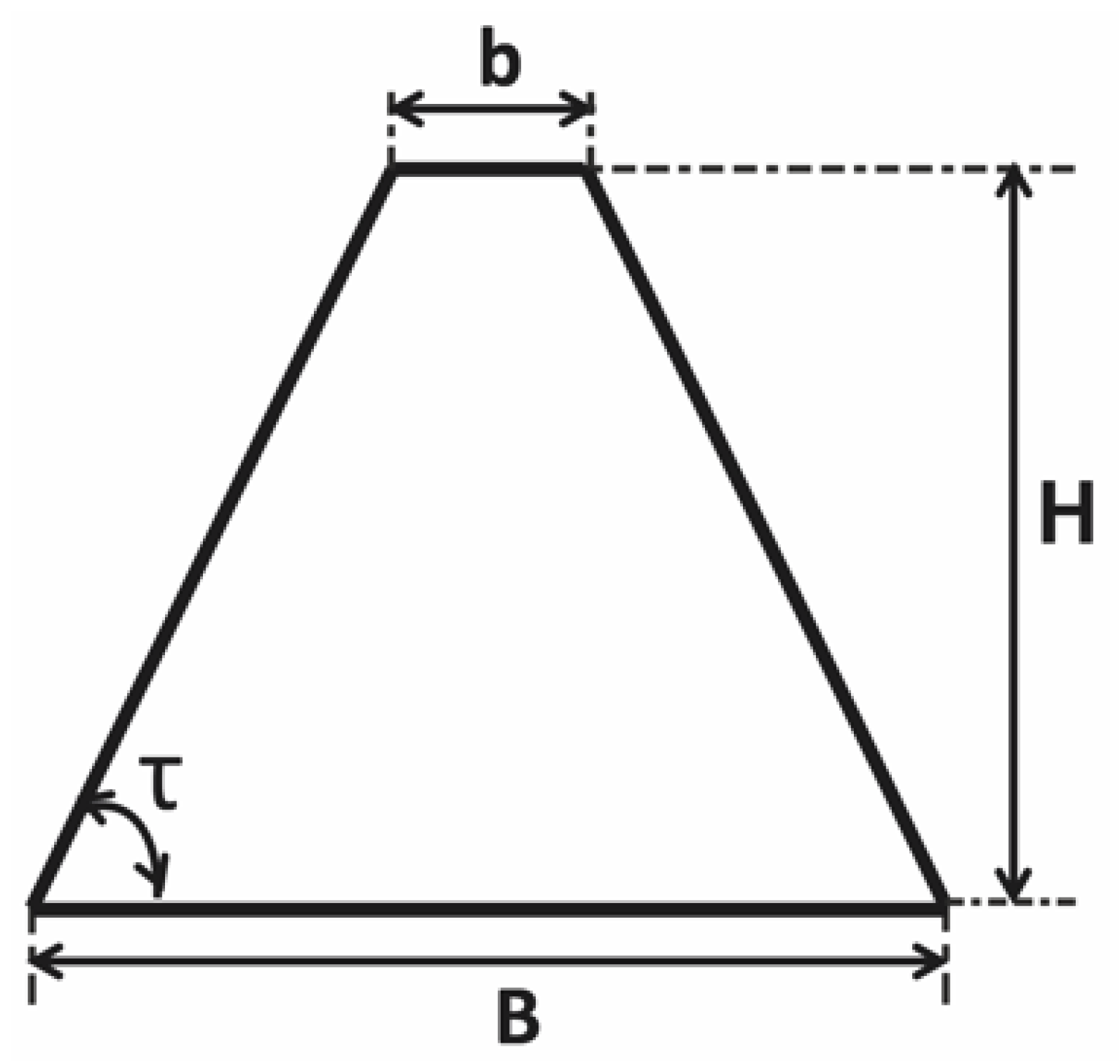
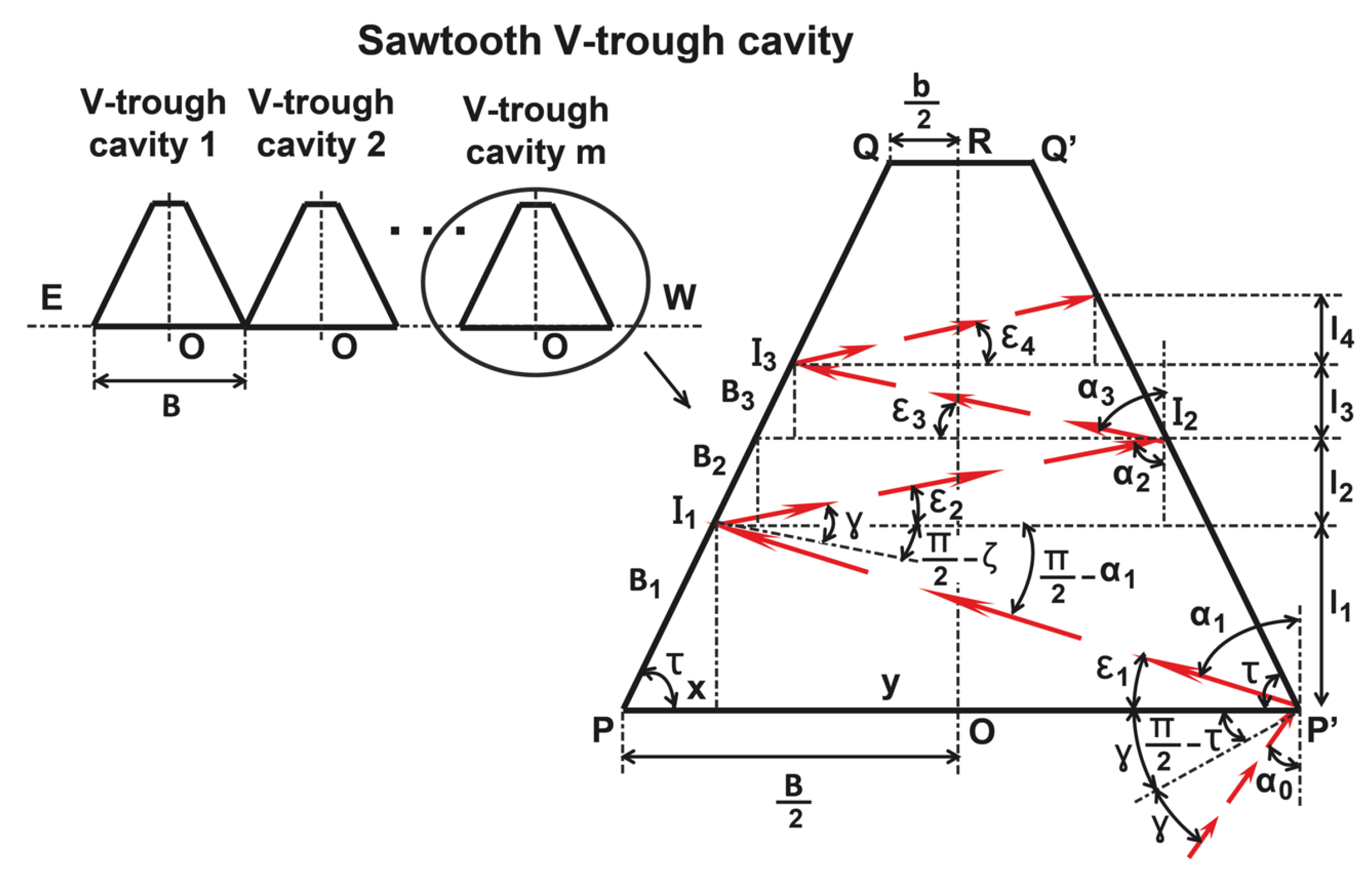
3.2. The Optimal Design of a Sawtooth V-Trough Cavity

The optimal design of the sawtooth V-trough cavity was developed based on analytical formulas. The sawtooth V-trough cavity presented here was formed by several V-trough cavities. The V-trough cavity parameters used in the design were: the width of the $PV$ cells (b), the aperture of the V-trough cavity (B), the height of the cavity (H), the trough wall angle ($\tau$), and the number of V-trough cavities in the sawtooth (m). The cross section of the sawtooth V-trough cavity presented in this paper is shown in Figure 5.

A classical V-shaped cavity (V-trough cavity m), as shown in Figure 5, was considered, and the assumptions made in this study were as follows:

(i)

The sawtooth V-trough cavity is symmetrical to the central mirror in the primary system.

(ii)

The sidewalls ($PQ$ and $P^{\prime }{Q}^{\prime }$) are assumed to be perfectly specular.

(iii)

The width of the $PV$ cells, b, is standardized by the $PV$ cell manufacturers.

(iv)

The V-trough cavity is east–west aligned.

(v)

The trough wall angle ($\tau$) is the complement of $\Phi$ [39].

(vi)

The trough wall angle ($\tau$) is fixed.

(vii)

The $OR$ axis is the reference axis for the angles of the sun’s incident rays. ${\theta }_i$ is considered positive for the solar rays coming from the mirrors on the left side and negative for those coming from the mirrors on the right.

(viii)

The angle between the solar ray reaching the cavity and $OR$ is denoted as ${\alpha }_0$ (i.e., ${\alpha }_0={\theta }_i$). In addition, each successive reflection of the sun’s ray inside the cavity is denoted as ${\alpha }_j$, for $j=1,2,\dots$

The sidewalls, $PQ$ and $P^{\prime }{Q}^{\prime }$, concentrate the beam of irradiance incident on the opening of the V-trough cavity ($P{P}^{\prime }$) onto the base of the V-trough cavity ($Q{Q}^{\prime }$). Four parameters were considered: the inlet beam solar irradiance, the trough wall angle ($\tau$), the aperture of the V-trough cavity (B), and the height of the cavity (H). The width of the $PV$ cells, $Q{Q}^{\prime }$, is not a free parameter, as it is set by the $PV$ cell manufacturers. As one of the objectives is for $100\%$ of the solar irradiation beam incident on the V-trough aperture to reach the $PV$ cells, the ray acceptance rate ${\eta }_{ray}$ must be 1; thus,

$$C_{opt}=C_a;\left|{\theta }_i\right|\le \left|{\theta }_c\right|,$$

(13)

where ${\theta }_i$ (°) is the angle of incidence of each ray coming from the different primary mirrors.

Since ${\eta }_{ray}=1$, B is maximized to find the maximum $C_a$ under the constraint that all solar rays reaching the cavity opening, $P{P}^{\prime }$, reach the photovoltaic cells (the width of which is b and is standardized by the $PV$ cell manufacturers) after a given number of reflections:

$$max{C}_a=maxB;\left|{\theta }_i\right|\le \left|{\theta }_c\right|.$$

(14)

The worst case scenario occurs when the solar ray coming from the mirrors on the left (right) side is reflected by $P^{\prime }$ (P) with ${\theta }_i={\theta }_c$. Figure 5 shows this scenario. Using the notation from Figure 5:

$${\theta }_i={\alpha }_0.$$

(15)

The following equality is obtained based on the Law of Reflection:

$${\alpha }_n=(\pi -2\tau )+{\alpha }_{n-1},$$

(16)

where n is the number of reflections inside the cavity needed to reach the $PV$ cells. Expressing Equation (16) as a function of ${\alpha }_0$:

$${\alpha }_n=n(\pi -2\tau )+{\alpha }_0.$$

(17)

The angle between $P{P}^{\prime }$ and the $i$-th reflection, ${\epsilon }_j$, can be calculated as:

$${\epsilon }_n=(2\tau -\pi /2)-{\alpha }_{n-1}.$$

(18)

In addition:

$${\epsilon }_n={\displaystyle \frac{\pi }{2}}-{\alpha }_n\Rightarrow tan{\alpha }_n=cot{\epsilon }_n.$$

(19)

The vertical lengths $l_i$ traveled by the reflected solar ray after each reflection can be calculated by the following equations:

$$l_n={\displaystyle \frac{B-2{\sum }_{i=1}^{n-1}\left(l_i\right)cot\tau }{cot\tau +tan{\alpha }_n}}.$$

(20)

The algorithm can be described, and an optimal design can be implemented with the equations developed above (14).

For the V-trough cavity design, the worst scenario occurs when the vertical component of each wall reflection (if there are any) is larger and touches the width of the $PV$ cells (b) at either Q or $Q^{\prime }$ [44]. Taking this fact into account, the iterative algorithm can be started by indicating a sequence of different scenarios $C_n$, for an increasing number of reflections n. The worst case condition is taken into account in each of these scenarios, ${\theta }_i={\theta }_c$. For each scenario $C_n$, the cavity height $H_n$, which is a function of B, can be calculated using (20):

$$H_n\left(B\right)={\sum }_{i=1}^n{l}_i.$$

(21)

The value of $H_n\left(B\right)$ can be substituted into the equation connecting the cavity parameters b, B, and H to $\tau$:

$$B=b+2H_n\left(B\right)cot\tau ,$$

(22)

and solving the above equation for B, after a few simple calculations:

$$\left(C_n\right)B_n\left(\tau \right)={(-1)}^{n}bcos({\alpha }_0-(2n+1)\tau )sec({\alpha }_0-\tau ).$$

(23)

One can see that the functions $B_n\left(\tau \right)$ are expressed in terms of b and ${\alpha }_0$. The algorithm concludes with the determination of the maximum value of $B_n\left(\tau \right)$ used to obtain the optimal angles ${\tau }_n^{*}$ that maximize B and, hence, $C_a$.

The algorithm makes it possible to choose the optimal design depending on the number of reflections n. Therefore, from a qualitative perspective, the use of a high number of reflections n, produces an increase in $B_n$, which means $C_a$ also increases. In fact, $C_a$ asymptotically moves toward the ideal value (8). In each scenario $C_n$, the number of reflections is n.

Lastly, to calculate the approximate value of n, one can use the property demonstrated by Shoeibi et al. [37]. This property indicates that the average number of reflections in a V-trough cavity is essentially the same as for compound parabolic concentrators ($CPCs$). Therefore, a truncated $CPC$ with the same height as the V-trough cavity can be considered, starting from an integer $CPC$ designed for the specific value of ${\theta }_c$. Note that the influence of n on the factor ${\rho }_m^n$ is quite small because ${\rho }_m$ is always very close to 1.

3.3. Uniform Distribution of Flux on PV Cells

A detailed study of the causes of the nonuniform illumination of $PV$ cells was presented in [18]. The wrong choice of some of the parameters, $d_i$, N, and $W_{Mi}$, produces this undesirable effect:

(i)

Parameter $d_i$ (small $d_i$). Shading (one mirror creates a shadow on an adjacent mirror) and blocking (one mirror blocks the reflected rays of an adjacent mirror) obviously depend on the distance between consecutive mirrors ($d_i$). This distance is not fixed and depends on the width of each mirror.

(ii)

Parameter $d_i$ (large $d_i$). Increasing the value of the parameter $d_i$ prevents the occurrence of the shading and blocking phenomena, but an excessive value of $d_i$ also leads to the nonuniform illumination of the $PV$ cells [18].

(iii)

Parameter N. As each mirror has a different $W_{Mi}$, using a large number of mirrors in the $SSLFR$ design increases the probability of a nonuniform flux distribution in the $PV$ cells [18].

(iv)

Parameter $W_{Mi}$. The ratio between the width of each mirror and the width of the $PV$ cells also influences the uniform illumination of the $PV$ cells [18].

As this research focuses on the design for a sawtooth V-trough cavity of an $SSLFR$, the algorithm proposed in [18] was used to design the primary reflector system. The optimum value of B was obtained once $W_{PV}$ ($b=W_{PV}$) was set by the manufacturer of the $PV$ cells; then, once the number of sawtooth V-trough cavities (m) was set, the design of the primary reflector system could begin.

It is not possible for $PV$ cells to be uniformly illuminated throughout the day. However, it is possible to determine a period of time, called the operation interval (${\theta }_{t_0}$), during which the $PV$ cells are uniformly illuminated, without any shading or blocking:

$${\theta }_t\in [-{\theta }_{t_0},{\theta }_{t_0}].$$

(24)

The following is fulfilled in the operation interval:

$$W_{fi}=W_{PV};1\le i\le N,$$

(25)

where the width of the $PV$ cells, $W_{PV}$, is a datum set by the manufacturer.

The operation interval can be determined by an iterative optimization algorithm [18]. A simplified method (graphical method) is proposed in this study based on the research in [18].

As the surface available for the installation of $SSLFRs$ is a key parameter [45], the width of the $SSLFR$ was a good starting point for the design thereof. The relationship between the width of the $SSLFR$ and the operation interval was obtained by applying the iterative optimization algorithm [18] for given values of b and m. Figure 6 shows the curve relating these parameters for: $b=30$ mm and ${\theta }_c=34$ (°) (a plausible value for the typical dimensions of an $SSLFR$ [18]) (therefore, $B=49.65$ mm), $m=4$, and various numbers of mirrors (5, 7, 9, and 11 mirrors). This number of mirrors was chosen so that the size of the $SSLFR$ would not be too large and the cost of the $SSLFR$ would not be too high (increasing the number of mirrors increases the cost of the $SSLFR$ [28]). Therefore, the operation interval was obtained once the width of the $SSLFR$ was fixed.

The position of the mirrors remained to be determined. A graph relating the position of the mirrors and the operation interval obtained by the iterative optimization algorithm proposed in [18] was also obtained. Figure 7 shows the curves relating the operation interval and the position of the mirrors.

The graph showing the relationship between the mirror width and the operation interval was obtained using the iterative optimization algorithm suggested in [18]. Figure 8 shows the curves relating the operation interval to the width of the mirrors.

Once ${\theta }_{t_0}$ was determined, it was also possible to determine the number of hours with a guaranteed homogeneous distribution of solar irradiance, without shading or blocking. The length of the operating interval is $I_{N_d}=[h_R(N_d,{\theta }_{t_0}),h_S(N_d,{\theta }_{t_0})]$, where $N_d$ is the day of the year. For example, Figure 9 represents the duration of the operating interval for several ${\theta }_{t_0}$ in Almeria (Spain) (latitude ${36}^{\circ }{50}^{\prime }{07}^{″}$ N, longitude ${02}^{\circ }{24}^{\prime }{08}^{″}$ W, and elevation 22 m).

The power reaching the $PV$ cells was estimated using the equation proposed by [18], as follows:

$$Q=\sum _{i=1}^{2·N+1}DNI·{\eta }_{opt}·L_{PV}·min\{W_{fi},W_{PV}\}·F_{bs}·cos{\theta }_i·cos{\theta }_l,$$

(26)

where $DNI$ is the direct normal irradiance (W/m${}^2$), ${\eta }_{opt}$ is the optical efficiency of the $SSLFR$ (this parameter groups together: the mirror reflectivity ($\rho$), the mirror cleanliness ($C{I}_m$), the glass cleanliness ($C{I}_g$), and the glass transmissivity (${\tau }_g$)), and the effectively illuminated length is $L_{PV}$. In addition, the full width of the $PV$ cell $W_{PV}$ is illuminated during the optimum operation time $I_{N_d}$. A shading and blocking factor $F_{bs}$ must be included, the value of which is 1 during the operating interval $I_{N_d}$ (there is none of either). The transverse angle ${\theta }_i$ between the normal to the i-th mirror and the incidence angle of the sun is:

$$cos{\theta }_i=cos({\beta }_i\pm {\alpha }_i),$$

(27)

with the configuration chosen in the longitudinal study:

$${\theta }_l={\theta }_z/2,$$

(28)

where ${\theta }_l$ is the longitudinal angle ($rad$), and ${\theta }_z$ is the zenith angle ($rad$).

Therefore, the power of the $SSLFR$ was determined for all hours of the operation interval $I_{N_d}$ and all days of the year $N_d$ as follows:

$$\sum _{N_d=1}^{365}{\int }_{h_R(N_d,{\theta }_{t_0})}^{h_S(N_d,{\theta }_{t_0})}Q·dT.$$

(29)

It is pertinent to remember the certainty that in this interval, there is neither shadow nor blockage, and the illumination is uniform.

3.4. Verification

For this paper, the SolTrace software, developed by the National Renewable Energy Laboratory ($NREL$), was used to validate the cavity, since it is currently one of the most widely used and recognized open source programs for the study of solar concentrators [18,46,47]. This software is based on the Monte Carlo ray-tracing methodology. In addition, SolTrace allows the assignment of parameters related to the reflection and refraction at the surface of the material. Another advantage of this software is that the user can specify a certain number of rays to be traced. The rays are generated randomly from the sun to the reflecting elements comprising the system, where the rays intersect. After optimizing the cavity, the determined geometrical parameters of both the cavity and the primary reflector system were entered into SolTrace to establish the geometrical model.

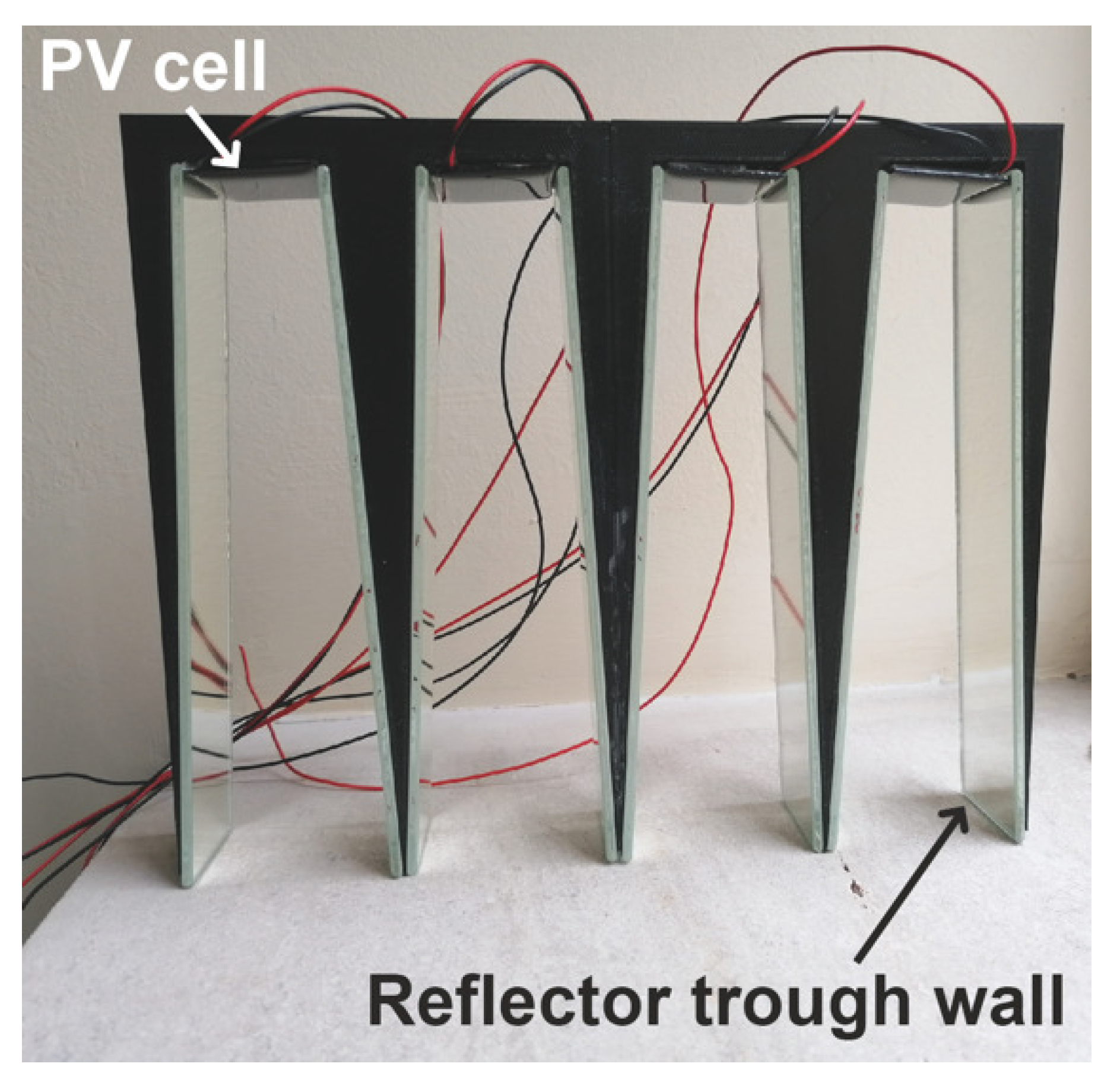
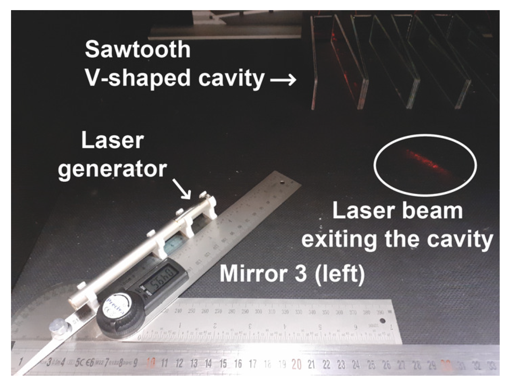
3.5. The Manufacture of the Sawtooth V-Trough Cavity and the Laser Experiment

The designed sawtooth V-trough cavity was manufactured based on 3D printing technology and additive manufacturing [22,48]. Additive manufacturing integrates computer-aided design, material processing, and molding technology [49]. The system used built a solid model of the sawtooth V-trough cavity by stacking special materials, in this case PLA, layer by layer, using software and a numerical control system on the basis of a digital model file [49]. The 3D printer used and a sawtooth V-trough cavity are shown in Figure 10. The cavity walls were covered with reflective mirrors.

A laser experimental platform for the verification of receiver cavities has been widely used [22,48,50]. Therefore, a laser experimental platform was also used for the study presented here.

An experimental test platform was constructed for ray-path control (see Figure 11). This experimental setup was mainly comprised of a level horizontal platform, a laser generator, a digital angle meter, an angle measuring device, and a metal scale. Similar devices were used in references [22,48,50]. The sensitive points of the test were as follows [22,48,50]: (i) to ensure that the equipment used remained perfectly fixed to the level horizontal platform, (ii) to ensure the levelness and stability of the horizontal platform by bubble leveling, (iii) to ensure that the laser generator was rigidly mounted on the rotating arm of the angle measuring device in such a way to maintain the laser generator parallel to the rotating arm, (iv) to provide a system for sliding the angle-measuring device along the metal scale and securing it to the scale by means of a locking device, and (v) to ensure the distance from the metal scale to the sawtooth V-trough cavity could be adjusted to simulate the position of any mirror in the primary reflector system.

In the experiment, the laser generator was adjusted to the position of each mirror by the angle of incidence and the position of the angle measuring device on the metal scale. Information on the position of the laser spot that formed when the light hit the reflecting wall of the cavity was recorded, and the position of the successive light reflections was checked.

4. Application of the Methodology and Analysis of the Results

It should be noted that this study is limited to small-scale linear Fresnel reflectors. Their small-scale characteristic is what allows longitudinal movement in the moving structure and the secondary reflector system. This ensures the uniform illumination of the photovoltaic cells from a longitudinal perspective.

The objective of this section is to verify the feasibility of the proposed methodology. The following parameters were used as a starting point in order to apply this methodology:

(i)

Available roof surface area. The available roof area was considered to be able to accommodate an $SSLFR$ with the following dimensions: width 2244 mm and length 2000 mm.

(ii)

Study location. The rooftop was located in Almería (Spain), for which the geographical data were: latitude 36°${50}^{\prime }07$${}^{″}$ N, longitude 02°${24}^{\prime }08$${}^{″}$ W, and altitude 22 m.

(iii)

Width of the commercial $PV$ cells ($W_{PV}=b$). A commercial $PV$ cell width of 30 mm was considered. The assumption of this value does not limit the application of the methodology.

(iv)

Acceptance angle (${\theta }_c$). A ${\theta }_c=34$ (°) was considered. It is a plausible value for the typical dimensions of an $SSLFR$ [18].

(v)

Number of V-trough cavities in the sawtooth (m). This m was equal to 4 to limit the number of mirrors as well as any increase in the cost of the $SSLFR$ [28]. Any other value of this parameter can be used.

(vi)

Height to the receiver (f). Usually, f takes the value of 1500 mm [18,35,36].

(vii)

Number of mirrors of the $SSLFR$. The number of mirrors of the $SSLFR$ was considered to be equal to seven so that the cost of the $SSLFR$ was not too high [28]. Therefore, $N=3$.

(viii)

Optical properties. The optical properties of the materials used were as follows [18]: the mirror reflectivity $\rho =$ $0.94$ [34], the mirror cleanliness $C{I}_m=0.96$ [51], the glass cleanliness $C{I}_g=0.96$ [51], and the glass transmissivity ${\tau }_g=0.92$ [52]. These optical properties were grouped into what is known as total optical yield (${\eta }_{opt}$).

Mathematica™ Computer Algebra System software was used to implement the optimization algorithm. This software has been widely used in similar studies [8,18]. The amount of direct solar irradiance on the horizontal surface of the site under study must be determined, i.e., the effect of the particular meteorological conditions must be taken into account. For this purpose, the method proposed by [53] was used. This method uses $PVGIS$ [54] data to obtain the monthly average direct solar irradiance.

The new cavity was compared to the standard V-trough cavity, keeping the cavity aperture, reflective surface area, and photovoltaic cell width constant. In addition, the focal height, number of mirrors, mirror width, and mirror spacing were also kept constant, so that the cost of the two configurations was the same from the point of view of the primary reflector system.

Table 1. Results of the sawtooth V-trough cavity.

	Parameters	Value
$C_a$	Area concentration ratio	$1.655$
${\tau }^{*}$	Trough wall angle	$87.00$°
B	Aperture of the V-trough cavity	$49.65$ mm
H	Height of the V-trough cavity	$187.47$ m

summarizes the results of the proposed optimization algorithm for the considered parameters.

Figure 12a shows the final design of the sawtooth V-trough cavity.

Using a single equivalent V-trough cavity and considering the same $PV$ cell surface and the same ${\theta }_c=34$ (°), the results shown in

Table 2. Results of the equivalent V-trough cavity.

	Parameters	Value
$C_a$	Area concentration ratio	$1.655$
${\tau }^{*}$	Trough wall angle	$87.00$ (°)
B	Aperture of the V-trough cavity	$198.6$ mm
H	Height of the V-trough cavity	$750.00$ (m)

were obtained. Figure 12b shows the final design of the equivalent V-trough cavity.

4.1. Comparison between the Proposed Sawtooth V-Cavity and the Standard V-Cavity

A comparison between the two cavities was made from various aspects, e.g., mechanical and thermal.

4.1.1. Mechanical Aspects

Comparing both designs, the height of the equivalent V-trough cavity was four times greater than the height of the sawtooth V-trough cavity. On the other hand, the refracting surface was the same in both cavities studied, in this case, $3.00$ m${}^2$; so, they would have the same $R_a$.

The method for calculating the wind load was defined in code CTE DB-SE-AE [55]. According to this code, the wind load is proportional to the exposure surface. The wind-exposed area of the equivalent V-trough cavity was four times larger than the sawtooth V-trough cavity. Therefore, the fixed structure and the secondary system of the $SSLFR$ would need to be reinforced to withstand four times higher wind loads. This considerably reduces the manufacturing cost of the $SSLFR$, as shown below:

(i)

Reduction in the cost of the fixed structure. As the height of the proposed cavity is much lower, the fixed structure of the $SSLFR$ is smaller, which lowers the cost thereof.

(ii)

Reduction in the cost of the fixed structure and secondary system structures. By reducing the height of the cavity, the surface area exposed to wind loads is smaller, which lowers the cost of the fixed structure and the secondary system structures.

4.1.2. Thermal Aspects

In the $PV$ cells, the part of the absorbed solar irradiance that is not converted into electricity is completely dissipated into heat, which represents an internal heat source that can be expressed as follows [56]:

$$Q_{th}=I_t·A_{PV}·(1-{\eta }_e),$$

(30)

where $Q_{th}$ is the internal heat generation in $PV$ cells (W), $I_t$ is the total absorbed solar irradiance for $PV$ cells (W/m${}^2$), ${\eta }_e$ is the electrical efficiency of the $PV$ system (%), and $A_{PV}$ is the total area of the $PV$ cells (m${}^2$). For the two cavities, the internal heat generation in $PV$ cells is the same, because they have the same number of $PV$ cells.

The heat transfer by conduction through the wall of the cooling system is determined by Fourier’s law of conduction through a hollow rectangular tube resulting from [57]:

$$Q_{th}=\frac{k·A_{ACS}·(T_{PV}-T_{ACS})}{{\delta }_{ACS}},$$

(31)

where k is the thermal conductivity (W/m °C), $A_{ACS}$ is the area of the active cooling system (m${}^2$), $T_{PV}$ is the temperature of the $PV$ cells (°C), $T_{ACS}$ is the temperature of the active cooling system $PV$ cells (°C), and ${\delta }_{ACS}$ is the wall thickness of the cooling system (m). As $Q_{th}$, k, and $\delta$ are equal for the two cavities, the area of the cooling system is inversely proportional to the $\Delta T$. The area of the cooling system in the case of the sawtooth V-cavity was $0.1789·L_{PV}$ (m${}^2$), and in the case of the standard V-cavity, it was $0.12·L_{PV}$ (m${}^2$). So, the cooling surface in the case of the sawtooth V-cavity was $1.49$ times larger. Therefore, the $\Delta T$ in the case of the sawtooth V-cavity was $0.67$ times the $\Delta T$ in the case of the standard V-cavity. Hence, the temperature of the $PV$ cells with the sawtooth V-cavity is always lower than that of PV cells with the standard V-cavity.

Figure 13 shows the relationship between the number of V-trough cavities of the sawtooth (m) and the width of the cooling system ($W_{ACS}$), keeping the width of the $PV$ cells constant ($W_{PV}$). One can see that this relationship was not linear. As m increased, the increase in the $W_{ACS}$ dropped.

According to Evans [58], the electrical efficiency of a photovoltaic cell depends on the temperature of the $PV$ cell:

$${\eta }_e={\eta }_{ref}·\left[1-{\beta }_{ref}·\left(T_{PV}-T_{ref}\right)\right],$$

(32)

where ${\eta }_{ref}$ is the electrical efficiency of the photovoltaic module at a reference temperature (dimensionless), ${\beta }_{ref}$ is the temperature coefficient (1/°C), $T_{PV}$ is the $PV$ cell temperature (°C), and $T_{ref}$ is the reference temperature (°C). Among other technical parameters, the manufacturer of the $PV$ module provides the value of ${\eta }_{ref}$ and ${\beta }_{ref}$. The ${\eta }_{ref}$ value normally refers to a temperature of 25 °C and a solar irradiance of 1000 (W/m${}^2$). Therefore, lowering the operating temperature of the $PV$ cells means increasing the electrical efficiency of the $PV$ cells.

4.1.3. Other Beneficial Aspects

Other beneficial aspects of the proposed cavity include:

(i)

The same reflective surface for both cavities. The multiple reflective walls of the new cavity, however, are used in combination to replace the two reflective surfaces of the V-trough cavity, which could reduce the difficulty of manufacturing, maintaining, and transporting the large glasses. This would also decrease the total cost of the $SSLFR$.

(ii)

The connection of the $PV$ cells. The connection of the photovoltaic cells is facilitated due to the separation between the photovoltaic cells in the new cavity.

4.2. The Application of the Graphic System When Designing the Primary Reflector System

Since the length of the $SSLFR$ was 2000 mm, the length of the mirrors was 2000 mm, and the length of the $PV$ cell system was also 2000 mm. As $N=3$, the graph shown in Figure 6b was used. On the $SSLFR$ width axis of the graph in Figure 6b, the value of 2244 mm was used, resulting in ${\theta }_{t_0}=50$° on the operation interval axis. Once the operation interval was known, the width of the mirrors was determined using the graph in Figure 7, and the position of the mirrors was determined using the graphs in Figure 8.

Table 3. Geometric values of the optimal design.

Mirror	${\mathit{L}}_{\mathit{i}}$ (mm)	${\mathit{W}}_{\mathit{Mi}}$ (mm)
Central mirror	0	$220.6$
Mirror 1 (right or left)	$323.5$	$228.3$
Mirror 2 (right or left)	$664.9$	$228.8$
Mirror 3 (right or left)	$1010.2$	$223.1$

shows the results obtained.

Using the $SSLFR$ parameters obtained previously, the annual energy of the sawtooth V-cavity was $2.38266$ MWh. The use of the new cavity did not lead to a decrease in the energy obtained.

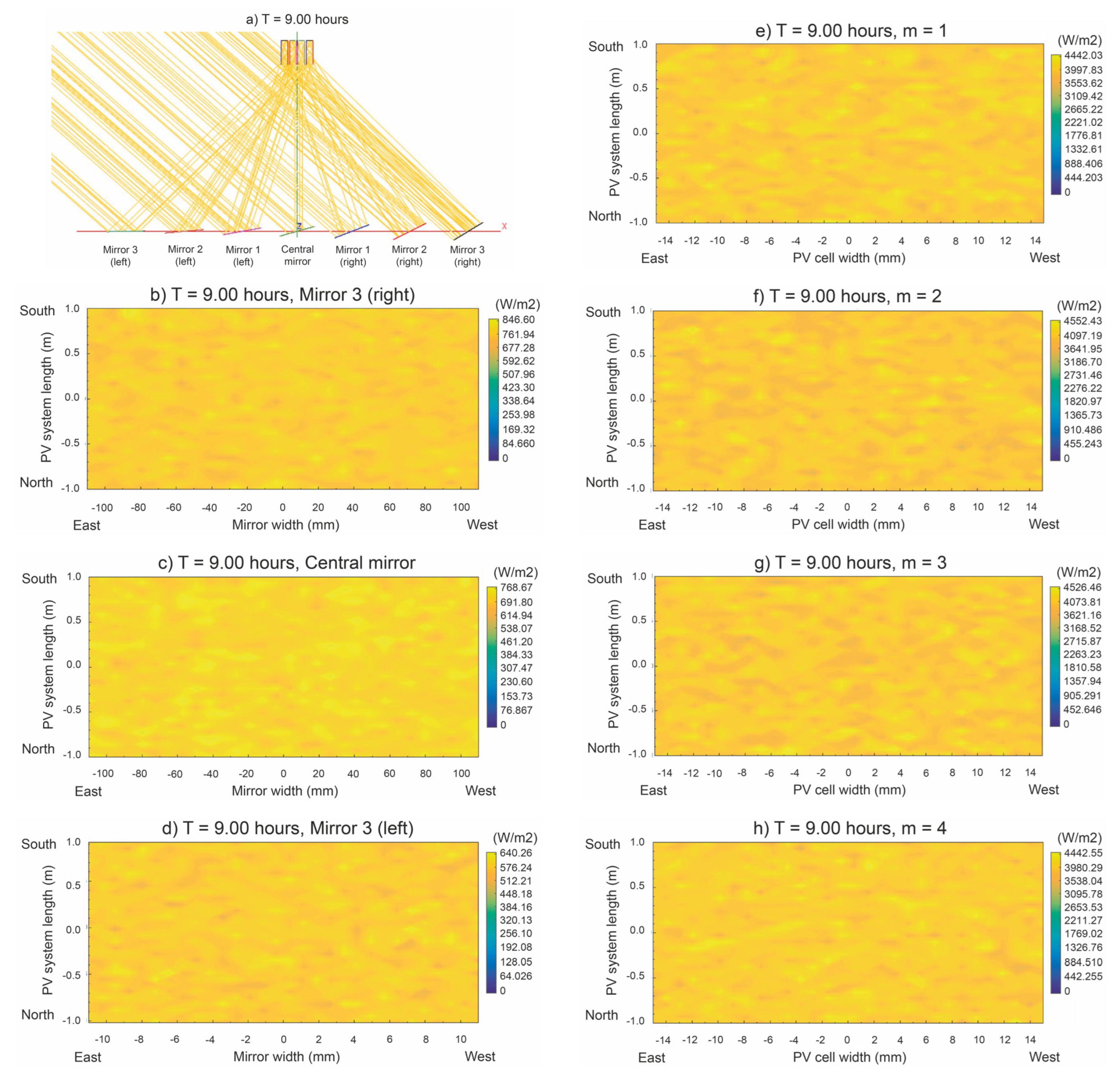
4.3. Verification through a Monte Carlo Simulation

A sawtooth V-trough cavity was optically modeled in this study. This design was verified using the Monte Carlo ray-tracing method. SolTrace™ is practical software that uses the Monte Carlo ray-tracing method. The application of this software has been used by several references for the optical analysis of solar concentrated systems [18,46,47]. Based on the results obtained previously, a model was implemented in the SolTrace™ software. Certain assumptions, common in this type of study, were made [18]: (i) all the reflective surfaces were flat and perfect; (ii) the errors in tracking the apparent movement of the sun were not considered; and (iii) the $SSLFR$ parameters shown in Table 1 and Table 3 were held constant. In total, ${10}^7$ rays were used for the simulations as recommended by other similar studies [18]. The direct normal irradiance for each day of the year was obtained by using the method presented by [53].

To verify the proposed design, the simulation time was during the summer solstice (day 172 of the year) at 9:00 (h) and 7:00 (h). The first simulation time chosen, T = 9:00 (h), belonged to the operation interval, where the $PV$ cells were uniformly illuminated. There was also no shading or blocking between adjacent mirrors. In contrast, the second simulation time chosen, T = 7:00 (h), did not belong to the operation interval.

The direct normal irradiance for the summer solstice at T = 9:00 (h) was $750.19$ (W/m${}^2$). Figure 14 shows some simulation results for different surfaces for the simulation time T = 9:00 (h). Figure 14a shows the absence of shading and blocking between the adjacent mirrors. This fact can also be seen in Figure 14b–d. Figure 14e–h show the surface of the $PV$ cells in the sawtooth V-trough cavity, where the flux density was completely homogeneous on the $PV$ cells.

The results of the flux density simulation on all the $SSLFR$ surfaces obtained with SolTrace are provided in

Table 4. Results of the flux density simulation at T = 9:00 (h).

Surface	Max. Irradiance W/m2	Min. Irradiance W/m2	Avg. Irradiance W/m2	Uniformity
Mirror 3 (right)	$846.60$	$668.60$	$749.17$	$0.033$
Mirror 2 (right)	$829.78$	$647.35$	$744.11$	$0.033$
Mirror 1 (right)	$804.10$	$651.78$	$728.44$	$0.035$
Central mirror	$768.67$	$631.41$	$701.40$	$0.035$
Mirror 1 (left)	$741.22$	$568.53$	$664.55$	$0.036$
Mirror 2 (left)	$693.40$	$543.74$	$622.32$	$0.036$
Mirror 3 (left)	$640.26$	$502.12$	$581.48$	$0.038$
$PV$ cell ($m=1$)	$4442.03$	$3357.50$	$3914.13$	$0.042$
$PV$ cell ($m=2$)	$4552.43$	$3461.41$	$3957.99$	$0.041$
$PV$ cell ($m=3$)	$4526.46$	$3402.96$	$3965.52$	$0.042$
$PV$ cell ($m=4$)	$4422.55$	$3279.57$	$3911.85$	$0.040$

. The SolTrace software output parameter called uniformity indicates the homogeneity of the flux density over the studied surface. The lower this parameter, the higher the homogeneity of the flux density. It can be seen that this parameter reflected very low values in the $PV$ cells. It is also true that the average value of the flux density over the photovoltaic cells was very similar. It should be noted that the minimum value of the flux density over the mirrors was different from 0, indicating the absence of shading and blocking between mirrors.

The direct normal irradiance for the summer solstice at T = 7:00 (h) was $656.53$ W/m${}^2$. Figure 15 shows some simulation results for different surfaces, for the simulation time T = 7:00 (h). These surfaces were the same as those studied in Figure 15. Figure 15a shows that mirrors 3 (right), 2 (right), 1 (right), central, and 1 (left) had different degrees of shading. This effect was more pronounced in mirror 3 (right), as the simulation time was before midday. Mirrors 2 (left) and 3 (left) had no shading. This fact can also be seen in Figure 15b–d. Figure 15e shows that the photovoltaic cell surface $m=1$ had a high degree of inhomogeneity. In contrast, the central $PV$ cells, $m=2$ and $m=3$, had a high degree of flux density homogeneity. The flux density homogeneity decreased for the $m=4$ $PV$ cell.

The results of the flux density simulation on all the $SSLFR$ surfaces obtained with SolTrace are provided in

Table 5. Results of the flux density simulation at T = 7:00 (h).

Surface	Max. Irradiance W/m2	Min. Irradiance W/m2	Avg. Irradiance W/m2	Uniformity
Mirror 3 (right)	$678.86$	0	$437.26$	$0.656$
Mirror 2 (right)	$681.67$	0	$440.10$	$0.615$
Mirror 1 (right)	$637.91$	0	$431.45$	$0.590$
Central mirror	$597.51$	0	$427.34$	$0.520$
Mirror 1 (left)	$559.36$	0	$451.93$	$0.333$
Mirror 2 (left)	$503.82$	$407.88$	$452.41$	$0.035$
Mirror 3 (left)	$450.52$	$362.43$	$407.87$	$0.035$
$PV$ cell ($m=1$)	$1859.69$	$238.63$	$827.51$	$0.433$
$PV$ cell ($m=2$)	$3789.32$	$2933.53$	$3409.21$	$0.037$
$PV$ cell ($m=3$)	$3793.43$	$3044.62$	$3418.47$	$0.034$
$PV$ cell ($m=4$)	$3727.6$	$2517.98$	$3193.99$	$0.074$

. The output parameter from the SolTrace software called uniformity reflected high values for the shaded mirrors and the $PV$ cell $m=1$, which had low flux density homogeneity. The average value of the flux density over the $PV$ cell $m=1$ was very low, indicating a lack of homogeneity in the flux density. In contrast, for the central $PV$ cells, $m=2$ and $m=3$, the average value of the flux density was very similar. The mirrors with a minimum flux density value of 0 had part of their surface shaded by an adjacent mirror.

To complete the comparative study between the sawtooth V-trough cavity and the equivalent V-trough cavity, Figure 16 shows the simulation time during the summer solstice (day 172 of the year) at 9:00 (h) of the equivalent V-trough cavity. Figure 16a shows the absence of shading and blocking between the adjacent mirrors. Figure 16b shows that the photovoltaic cell surface had a high degree of inhomogeneity. In contrast, for the same hour, the sawtooth V-cavity flux density was completely homogeneous in the $PV$ cells.

The results of the flux density simulation on all the $SSLFR$ surfaces obtained with SolTrace are provided in

Table 6. Results of the flux density simulation at T = 9:00 (h) in the equivalent V-trough cavity.

Surface	Max. Irradiance W/m2	Min. Irradiance W/m2	Avg. Irradiance W/m2	Uniformity
Mirror 3 (right)	$888.06$	$623.43$	$749.38$	$0.048$
Mirror 2 (right)	$852.34$	$659.14$	$742.37$	$0.044$
Mirror 1 (right)	$839.35$	$625.05$	$728.45$	$0.048$
Central mirror	$808.51$	$597.45$	$702.83$	$0.048$
Mirror 1 (left)	$806.88$	$564.98$	$664.39$	$0.051$
Mirror 2 (left)	$738.70$	$513.03$	$623.30$	$0.049$
Mirror 3 (left)	$660.71$	$480.56$	$581.40$	$0.05$
$PV$ cell	$2102.45$	$600.71$	$1184.97$	$0.38$

for the equivalent V-trough cavity. Comparing Table 4 and Table 6, we see there were similar values of incident solar irradiance on the mirrors, and a considerable reduction in the incident solar irradiance on the PV cells in the case of the equivalent V-trough cavity. The high value of the uniformity parameter indicated the non-homogeneity of the photovoltaic cells in the equivalent V-trough cavity. The opposite was the case with the sawtooth V-trough cavity.

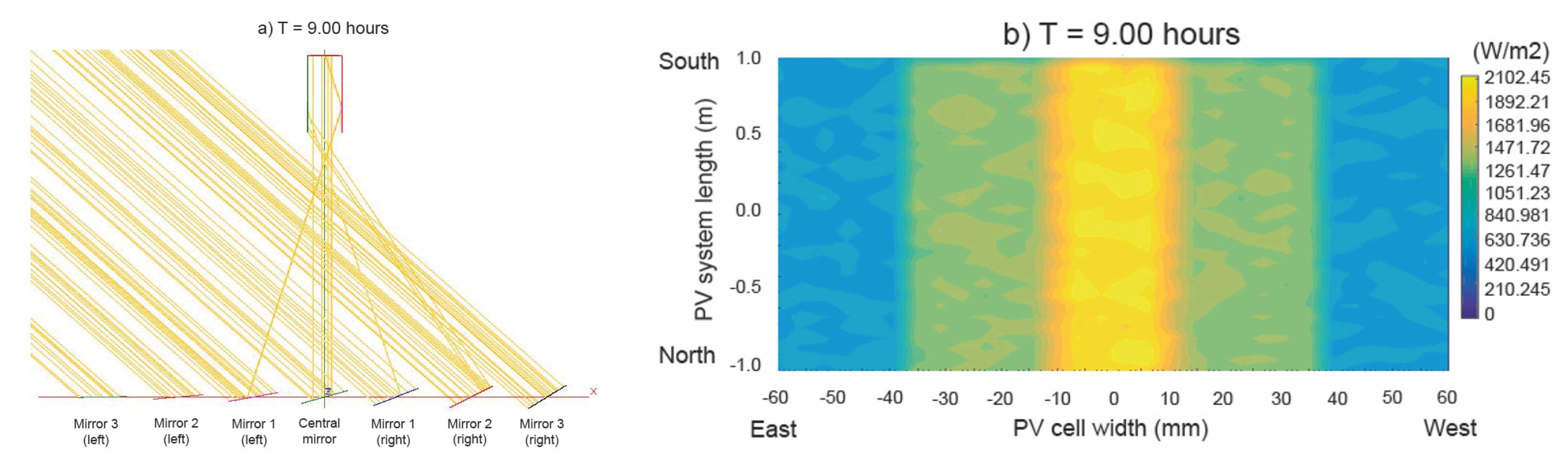
4.4. Influence of the Acceptance Angle of the V-Trough Cavity

In the previous sections, a case was presented in which the acceptance angle of the V-trough cavity ${\theta }_c=34$ (°) was considered. This value corresponded to an $SSLFR$ with a width of 2244 mm and a number of mirrors equal to seven ($N=3$). The value of ${\theta }_c$ came from a focal length $f=1500$ mm and from the center of the mirror 3 (right or left), whose center, as we saw, was at a distance of $L_3=1010.2$ mm (see Table 3).

In this section, the influence of the V-trough cavity acceptance angle is analyzed. For this purpose, several simulations were carried out, varying ${\theta }_c\in [22,46]$ (°), obtaining the results shown in Figure 17. Figure 17a shows the variation in $C_a$. Considering the absorber width $b=30$ mm, the variation in B is shown in Figure 17b, and the variation in H is shown in Figure 17c.

As shown in Figure 17, as the acceptance angle increased, the geometric concentration ratio decreased nonlinearly. This variation translated almost linearly (obviously) to the value of B and almost linearly also to H. The latter result is due to the fact that the optimal value ${\tau }^{*}$ of the trough wall angle also showed a linear variation with ${\theta }_c$, with values ranging from $86.4$ to $87.6$ (°) for the range of the variation in ${\theta }_c$.

As discussed below, the variation in the acceptance angle had an influence on the design of the $SSLFR$, as it directly affects the secondary reflector system and, therefore, the primary reflector system.

From the point of view of the secondary reflector, this variation in $C_a$ led to the following situation. Once b was set by the manufacturer of the $PV$ cells, the optimum value of B was obtained. Since the commercial cells used in this work had a fixed value of $b=30$ mm, in the base case already analyzed, with ${\theta }_c=34$°, and a number of V-trough cavities of the sawtooth $m=4$, we were guaranteed a swept width of the entire secondary of $4B\simeq 200$ mm. If we then considered a smaller ${\theta }_c$ value, as $C_a$ grew, there came a point where, with a smaller number of V-trough cavities of the sawtooth, in this case, $m=3$, we achieved the same sweep of the secondary $3B\simeq 200$ mm. This was achieved for ${\theta }_c=23$°. Similarly, by increasing ${\theta }_c$, and decreasing $C_a$, it was necessary to take $m=5$, in order to have the same sweep of the secondary $5B\simeq 200$ mm. This situation occurred for ${\theta }_c=46$°.

Table 7. Results of the influence of the acceptance angle on some parameters of the SSLFR.

Secondary Reflector System				Primary Reflector System
${\mathit{\theta }}_{\mathit{c}}$ (°)	${\mathit{C}}_{\mathit{a}}$	$\mathit{B}$ (mm)	$\mathit{m}$	$\mathit{N}$	${\mathit{L}}_{\mathit{N}}$ (mm)	${\mathit{\theta }}_{\mathit{to}}$ (°)
23	$2.22$	$66.66$	3	2	640	49
34	$1.66$	50	4	3	1010	50
46	$1.33$	40	5	5	1550	47

shows the influence of the variation in the acceptance angle with respect to the parameters of the secondary reflector system.

The variation in the acceptance angle also influenced the design of the primary reflector system. Considering $f=1500$ mm, the three cases that were analyzed induced changes in the main parameters of the primary reflector system. Table 7 shows the influence of the variation in the acceptance angle with respect to the parameters of the primary reflector system.

When ${\theta }_c=34$ (°), the base case, the optimal design corresponded to ${\theta }_{to}=50$ (°), $N=3$, and $L_N=1010$ mm.

When the acceptance angle decreased, e.g., ${\theta }_c=23$°, to achieve that angle and a very similar operating range of ${\theta }_{to}=49$°, the mirror field of the primary had the following parameters: $N=2$ and $L_N=640$ mm. In contrast, when the acceptance angle increased, for example, ${\theta }_c=46$° and a very similar operating range ${\theta }_{to}=47$°, the mirror field of the primary had the following parameters: $N=5$ and $L_N=1550$ mm.

Comparing the three cases, and considering the variation in ${\theta }_{to}$ to be negligible, the case ${\theta }_c=46$° significantly increased the area of the primary field of mirrors; therefore, this case increased the number of $PV$ cells, the solar irradiation received, and the cost of the $SSLFR$. On the other hand, in the case ${\theta }_c=23$°, the situation was the opposite: fewer $PV$ cells, a lower solar irradiation received, and a lower cost of the $SSLFR$. Therefore, several factors must be taken into account in the choice of the acceptance angle, such as the economic factor, the energy factor, and the surface area available for the installation of the $SSLFR$.

4.5. The Manufacture of the Sawtooth V-Trough Cavity and the Laser Experiment

The sawtooth V-trough cavity was constructed using a biodegradable green polymer material known as polylactic acid ($PLA$), with the dimensions shown in Figure 12a. The photograph of the sawtooth V-trough cavity presented in this paper is shown in Figure 18.

As the dimensions of the experimental test platform were smaller than the dimensions of the $SSLFR$, the position of the $SSLFR$ mirrors and the height to the receiver were scaled. The width of the mirrors and the angle of incidence were not affected.

Table 8. Optimal parameters scaled to the experimental test platform.

Mirror	${\mathit{L}}_{\mathit{i}}$ (mm)	${\mathit{W}}_{\mathit{Mi}}$ (mm)	${\mathit{\theta }}_{\mathit{i}}$ (°)
Central mirror	0	$220.6$	0
Mirror 1 (right or left)	$61.0$	$228.3$	$12.17$
Mirror 2 (right or left)	$125.4$	$228.8$	$23.90$
Mirror 3 (right or left)	$205.2$	$223.1$	$33.95$

shows the optimal parameters scaled to the experimental test platform; in this case, $f=283$ mm. The laser generator was placed in three positions for each mirror tested: an extreme left position, a central position, and an extreme right position.

Figure 19a shows the laser beam emitted by the laser generator, starting from the extreme left position of the mirror 2 (left) with an angle of incidence of $23.90$°. As expected, the beam was incident on the cavity $m=1$. Figure 19b shows the laser beam emitted by the laser generator, starting from the extreme right position of the mirror 2 (left) with an angle of incidence of $23.90$° (the maximum acceptance angle that corresponds to that mirror due to the geometry of the $SSLFR$). As expected, the beam was incident on the cavity $m=4$. These results indicate that the ray acceptance rate is 1. The rest of the tests carried out for the other mirrors also showed that the laser beam hit the $PV$ cell. The experimental results obtained using the cavity designed showed that the constructed cavity met the set conditions.

The angle measured with the digital angle meter did not match the actual angle of the laser beam when it reached the reflecting surface of the cavity. There are several reasons for this: (i) The laser beam emitted by the laser generator has a certain divergence [50], since the laser is deflected as the optical length increases. (ii) The laser beam emitted by the laser generator is not an absolutely parallel beam [50], which causes the beam spot to reach the surface at a slightly different angle. Therefore, the angle of incidence of the laser beam is affected. In general, these sources of error are considered to have a cumulative effect and do not cancel each other out [50]. However, as the distance from the laser generator to the cavity was 349 mm in the worst case of mirror 3 (left or right), this angle error was considered to be within a reasonable range [48,50].

Figure 20 shows the laser beam emitted by the laser generator, starting from the extreme left position of the mirror 3 (left) with an angle of incidence of $35.00$°. As can be seen in this image, the laser beam exited the cavity.

5. Conclusions

Guaranteeing the uniformity of the solar irradiance distribution in photovoltaic cells is a major issue in concentrating photovoltaic systems based on a small-scale linear Fresnel reflector. For this purpose, a new cavity design for a low-concentration photovoltaic system based on a small-scale linear Fresnel reflector was proposed to decrease the height thereof while maintaining a constant aperture. The design of a sawtooth V-cavity that maintained the ray acceptance rate at 1 and the uniform distribution of the solar irradiance on the photovoltaic cells was calculated analytically using an optimization algorithm. The analytical approach presented provides equations for any number of reflections inside the cavity, which are easily implemented as an iterative algorithm. The proposed design was verified using the Monte Carlo ray-tracing method. SolTrace™ software was used for this purpose. In order to verify the correct sawtooth V-trough cavity design, a prototype was built with a biodegradable green polymer material known as polylactic acid (PLA) using 3D printing technology. An experimental laser platform was built to fix the trajectory of the laser beam to confirm that the ray acceptance rate was 1, i.e., that all the beams entering the cavity reached the photovoltaic cells. The proposed sawtooth V-trough cavity was compared with the standard V-trough cavity, keeping the cavity aperture, reflective surface area, and photovoltaic cell width constant. In addition, the focal height, number of mirrors, mirror width, and mirror spacing were also kept constant, so that the cost of the two configurations was the same from the point of view of the primary reflector system. In the example analyzed, the annual energy of the sawtooth V-trough cavity was $2.38266$ MWh. The new design ensured the uniform distribution of the solar irradiation and significantly reduced the height of the cavity. This achievement considerably reduces the manufacturing cost of the small-scale linear Fresnel reflectors, as shown below:

(i)

Since the height of the proposed cavity is much lower, in this case four times lower, the fixed structure of the small-scale linear Fresnel reflectors are smaller; therefore, the cost is lower.

(ii)

The wind-exposed area of the sawtooth V-trough cavity is four times less than in the case of the standard V-trough cavity, which reduces the cost of the fixed structure and secondary system structures. This is essential considering that the optimal installation location for small-scale linear Fresnel reflectors is on the roofs of buildings.

(iii)

The cooling surface in the case of the sawtooth V-cavity is $1.49$ times larger, and the $\Delta T$ in the case of the sawtooth V-cavity is $0.67$ times the $\Delta T$ in the case of the standard V-cavity. Hence, the temperature of the $PV$ cells with the sawtooth V-cavity is always lower than that of $PV$ cells with a standard V-cavity, which increases the electrical efficiency.

(iv)

Although both cavities have the same reflective surface, the multiple reflective walls of the new cavity are used in combination to replace the two reflective surfaces of the standard V-trough cavity, which could reduce the difficulty in manufacturing, maintaining, and transporting the large glasses. Furthermore, the overall cost of the small-scale linear Fresnel reflector may also decrease.

Other beneficial aspects of the proposed cavity include:

(v)

Although the surface area of the photovoltaic cells is the same, the spacing between the photovoltaic cells that characterizes the designed cavity facilitates cooling between the photovoltaic cells and the use of cooling systems with a larger surface area, which improves the efficiency of the cooling system.

(vi)

Due to the separation between the photovoltaic cells in the new cavity, the connection between the photovoltaic cells is easier.

Finally, we also presented an innovative graphic system to design the primary reflector system for the small-scale linear Fresnel reflector. All of this makes it possible for users to quickly and easily make the necessary calculations without needing to program formulas.

References

1. Yadav, P.; Tripathi, B.; Lokhande, M.; Kumar, M. Estimation of steady state and dynamic parameters of low concentration photovoltaic system. Sol. Energy Mater. Sol. Cells 2013, 112, 65–72. [Google Scholar]
2. IRENA. Future of Solar Photovoltaic: Deployment, Investment, Technology, Grid Integration and Socio-Economic Aspects; International Renewable Energy Agency: Abu Dhabi, United Arab Emirates, 2019; Available online: https://irena.org/-/media/Files/IRENA/Agency/Publication/2019/Nov/IRENA_Future%_of_Solar_PV_2019.pdf (accessed on 11 June 2023).
3. Barbose, G.; Darghouth, N.; O’Shaughnessy, E.; Forrester, S. Tracking the Sun: Pricing and Design Trends for Distributed Photovoltaic Systems in the United States; Lawrence Berkeley National Laboratory: Berkeley, CA, USA, 2021.
4. IRENA. Solar Costs To Fall Further, Powering Global Demand; International Renewable Energy Agency: Abu Dhabi, United Arab Emirates, 2017; Available online: https://www.reuters.com/article/singapore-energy-solar-idUSL4N1MY2F8 (accessed on 11 June 2023).
5. Pvinsights. Available online: http://pvinsights.com/ (accessed on 11 June 2023).
6. IRENA; IEA. End-of-Life Management: Solar Photovoltaic Panels; International Renewable Energy Agency: Abu Dhabi, United Arab Emirates; International Energy Agency Photovoltaic Power Systems: Paris, France, 2016; Available online: https://www.irena.org/publications/2016/Jun/End-of-life-management-Solar-Photovoltaic-Panels (accessed on 11 June 2023).
7. Hasan, H.A.; Sopian, K.; Jaaz, A.H.; Al-Shamani, A.N. Experimental investigation of jet array nanofluids impingement in photovoltaic/thermal collector. Sol. Energy 2017, 144, 321–334. [Google Scholar] [CrossRef]
8. Barbón, A.; Bayón-Cueli, C.; Bayón, L.; Fortuny Ayuso, P. Influence of solar tracking error on the performance of a small-scale linear Fresnel reflector. Renew. Energy 2020, 162, 43–54. [Google Scholar] [CrossRef]
9. Barbón, A.; Fernández-Rubiera, J.A.; Martínez-Valledor, L.; Pérez-Fernández, A.; Bayón, L. Design and construction of a solar tracking system for small-scale linear Fresnel reflector with three movements. Appl. Energy 2021, 285, 116477. [Google Scholar]
10. Kandilli, C. Performance analysis of a novel concentrating photovoltaic combined system. Energy Convers. Manag. 2013, 67, 186–196. [Google Scholar]
11. Barbón, A.; Ghodbane, M.; Bayón, L.; Said, Z. A general algorithm for the optimization of photovoltaic modules layout on irregular rooftop shapes. J. Clean. Prod. 2022, 365, 132774. [Google Scholar] [CrossRef]
12. Silva, R.M.; Fernandes, J.L.M. Hybrid photovoltaic/thermal (PV/T) solar systems simulation with Simulink/Matlab. Sol. Energy 2010, 84, 1985–1996. [Google Scholar] [CrossRef]
13. Kamath, H.G.; Ekins-Daukes, N.J.; Araki, K.; Ramasesha, S.K. The potential for concentrator photovoltaics: A feasibility study in India. Prog. Photovoltaics Res. Appl. 2018, 27, 316–327. [Google Scholar] [CrossRef]
14. Moreno, A.; Chemisana, D.; Fernández, E.F. Hybrid high-concentration photovoltaic-thermal solar systems for building applications. Appl. Energy 2021, 304, 117647. [Google Scholar] [CrossRef]
15. Bamroongkhan, P.; Lertsatitthanakorn, C.; Soponronnarit, S. Experimental performance study of a solar parabolic dish photovoltaic-thermoelectric generator. Energy Procedia 2019, 158, 528–533. [Google Scholar] [CrossRef]
16. Brahim Kechiche, O.B.H.; Hamza, M. Enhancement of a commercial PV module performance under low concentrated photovoltaic (LCPV) conditions: A numerical study. Renew. Energy Focus 2022, 41, 258–267. [Google Scholar]
17. Xu, N.; Ji, J.; Sun, W.; Huang, W.; Li, J.; Jin, Z. Numerical simulation and experimental validation of a high concentration photovoltaic/thermal module based on point-focus Fresnel lens. Appl. Energy 2016, 168, 269–281. [Google Scholar]
18. Barbón, A.; Fortuny Ayuso, P.; Bayón, L.; Fernández-Rubiera, J.A. Non-uniform illumination in low concentration photovoltaic systems based on small-scale linear Fresnel reflectors. Energy 2022, 239, 122217. [Google Scholar]
19. Wang, G.; Wang, F.; Shen, F.; Jiang, T.; Chen, Z.; Hu, P. Experimental and optical performances of a solar CPV device using a linear Fresnel reflector concentrator. Renew. Energy 2020, 146, 2351–2361. [Google Scholar] [CrossRef]
20. Said, Z.; Ghodbane, M.; Kumar Tiwari, A.; Muhammad Ali, H.; Boumeddane, B.; Ali, Z.M. 4E (Energy, Exergy, Economic, and Environment) examination of a small LFR solar water heater: An experimental and numerical study. Case Stud. Therm. Eng. 2021, 27, 101277. [Google Scholar]
21. Vihari Parupudi, R.; Singh, H.; Kolokotroni, M. Low Concentrating Photovoltaics (LCPV) for buildings and their performance analyses. Appl. Energy 2020, 279, 115839. [Google Scholar]
22. Xu, J.; Chen, F.; Xia, E.; Gao, C.; Deng, C. An optimization design method and optical performance analysis on multi-sectioned compound parabolic concentrator with cylindrical absorber. Energy 2020, 197, 117212. [Google Scholar]
23. Ustaoglu, A.; Ozbey, U.; Torlaklı, H. Numerical investigation of concentrating photovoltaic/thermal (CPV/T) system using compound hyperbolic–trumpet, V-trough and compound parabolic concentrators. Renew. Energy 2020, 152, 1192–1208. [Google Scholar]
24. Otanicar, T.P.; Wingert, R.; Orosz, M.; McPheeters, C. Concentrating photovoltaic retrofit for existing parabolic trough solar collectors: Design, experiments, and levelized cost of electricity. Appl. Energy 2020, 265, 11475. [Google Scholar]
25. Al-Shohani, W.A.M.; Al-Dadah, R.; Mahmoud, S.; Algareu, A. Optimum design of V-trough concentrator for photovoltaic applications. Sol. Energy 2016, 140, 241–254. [Google Scholar]
26. Barbón, A.; Sánchez Rodríguez, J.A.; Bayón, L.; Barbón, N. Development of a fiber daylighting system based on a small scale linear Fresnel reflector: Theoretical elements. Appl. Energy 2018, 212, 733–745. [Google Scholar] [CrossRef]
27. Pardellas, A.; Fortuny Ayuso, P.; Bayón, L.; Barbón, A. A new two-foci V-trough concentrator for small-scale linear Fresnel reflectors. Energies 2023, 16, 1597. [Google Scholar] [CrossRef]
28. Barbón, A.; Sánchez-Rodríguez, J.A.; Bayón, L.; Bayón-Cueli, C. Cost estimation relationships of a small scale linear Fresnel reflector. Renew. Energy 2019, 134, 1273–1284. [Google Scholar] [CrossRef]
29. Li, G.; Xuan, Q.; Pei, G.; Su, Y.; Ji, J. Effect of non-uniform illumination and temperature distribution on concentrating solar cell—A review. Energy 2018, 144, 1119–1136. [Google Scholar] [CrossRef]
30. Guerriero, P.; Tricoli, P.; Daliento, S. A bypass circuit for avoiding the hot spot in PV modules. Sol. Energy 2019, 181, 430–438. [Google Scholar] [CrossRef]
31. Ustaoglu, A.; Kandilli, C.; Cakmak, M.; Torlaklı, H. Experimental and economical performance investigation of V-trough concentrator with different reflectance characteristic in photovoltaic applications. J. Clean. Prod. 2020, 272, 123072. [Google Scholar] [CrossRef]
32. Ghodbane, M.; Said, Z.; Amine Hachicha, S.; Boumeddane, B. Performance assessment of linear Fresnel solar reflector using MWCNTs/DW nanofluids. Renew. Energy 2020, 151, 43–56. [Google Scholar] [CrossRef]
33. Barbón, A.; Barbón, N.; Bayón, L.; Sánchez-Rodríguez, J.A. Parametric study of the small-scale linear Fresnel reflector. Renew. Energy 2018, 116, 64–74. [Google Scholar] [CrossRef]
34. Duffie, J.A.; Beckman, W.A. Solar Engineering of Thermal Processes; John Wiley & Sons: Hoboken, NJ, USA, 2013. [Google Scholar]
35. Zhu, Y.; Shi, J.; Li, Y.; Wang, L.; Huang, Q.; Xu, G. Design and thermal performances of a scalable linear Fresnel reflector solar system. Energy Convers. Manag. 2017, 146, 174–181. [Google Scholar] [CrossRef]
36. Zhu, Y.; Shi, J.; Li, Y.; Wang, L.; Huang, Q.; Xu, G. Design and experimental investigation of a stretched parabolic linear Fresnel reflector collecting system. Energy Convers. Manag. 2016, 126, 89–98. [Google Scholar] [CrossRef]
37. Shoeibi, H.; Jarrahian, A.; Mehrpooya, M.; Assaerh, E.; Izadi, M.; Pourfayaz, F. Mathematical modeling and simulation of a compound parabolic concentrators collector with an absorber tube. Energies 2023, 16, 287. [Google Scholar] [CrossRef]
38. Jaaz, A.H.; Abdulrasool Hasan, H.; Sopian, K.; Haji Ruslan, M.H.B.; Hussain Zaidi, S. Design and development of compound parabolic concentrating for photovoltaic solar collector: Review. Renew. Sustain. Energy Rev. 2017, 76, 1108–1121. [Google Scholar] [CrossRef]
39. Tina, G.M.; Scandura, P.F. Case study of a grid connected with a battery photovoltaic system: V-trough concentration vs. single-axis tracking. Energy Convers. Manag. 2012, 64, 569–578. [Google Scholar] [CrossRef]
40. Hadavinia, H.; Harjit, S. Modelling and experimental analysis of low concentrating solar panels for use in building integrated and applied photovoltaic (BIPV/BAPV) systems. Renew. Energy 2019, 139, 815–829. [Google Scholar] [CrossRef]
41. Madala, S.; Boehm, R.F. A review of nonimaging solar concentrators for stationary and passive tracking applications. Renew. Sustain. Energy Rev. 2017, 71, 309–322. [Google Scholar] [CrossRef]
42. Oprea, R.; Istrate, M.; Machidon, D. Analysis of V-trough reflector’s geometry influence on low concentration photovoltaic systems. In Proceedings of the 8th International Conference on Modern Power Systems, Cluj-Napoca, Romania, 21–23 May 2019. [Google Scholar]
43. Tang, R.; Liu, X. Optical performance and design optimization of V-trough concentrators for photovoltaic applications. Sol. Energy 2011, 85, 2154–2166. [Google Scholar] [CrossRef]
44. Fernández-Rubiera, J.A.; Barbón, A.; Bayón, L.; Díaz, G.; Bayón-Cueli, C. Low concentration photovoltaic systems based on small-scale linear Fresnel reflectors: Development of a new sawtooth V-trough concentrator. In Proceedings of the IEEE International Conference on Environmental and Electrical Engineering (EEEIC2022), Prague, Czech Republic, 8 June–1 July 2022; pp. 1–6. [Google Scholar]
45. Barbón, A.; Barbón, N.; Bayón, L.; Sánchez-Rodríguez, J.A. Optimization of the distribution of small scale linear Fresnel reflectors on roofs of urban buildings. Appl. Math. Model. 2018, 59, 233–250. [Google Scholar] [CrossRef]
46. Mishra, P.; Pandey, M.; Tamaura, Y.; Tiwari, S. Numerical analysis of cavity receiver with parallel tubes for cross-linear concentrated solar system. Energy 2021, 220, 119609. [Google Scholar] [CrossRef]
47. Gong, J.H.; Wang, J.; Lund, P.D.; Zhao, D.D.; Hu, E.Y. Improving the performance of large-aperture parabolic trough solar concentrator using semi-circular absorber tube with external fin and flat-plate radiation shield. Renew. Energy 2022, 159, 1215–1223. [Google Scholar] [CrossRef]
48. Xu, J.; Chen, F.; Deng, C. Design and analysis of a novel multi-sectioned compound parabolic concentrator with multi-objective genetic algorithm. Energy 2021, 225, 120216. [Google Scholar] [CrossRef]
49. Tan, L.J.; Zhu, W.; Zhou, K. Recent progress on polymer materials for additive manufacturing. Adv. Funct. Mater. 2020, 30, 2003062. [Google Scholar] [CrossRef]
50. Chen, F.; Liu, Y. Model construction and performance investigation of multi-section compound parabolic concentrator with solar vacuum tube. Energy 2022, 250, 123887. [Google Scholar] [CrossRef]
51. Sharma, V.M.; Nayak, J.K.; Kedare, S.B. Effects of shading and blocking in linear Fresnel reflector field. Sol. Energy 2015, 113, 114–138. [Google Scholar] [CrossRef]
52. Theunissen, P.H.; Beckman, W.A. Solar transmittance characteristics of evacuated tubular collectors with diffuse back reflectors. Sol. Energy 1985, 35, 311–320. [Google Scholar] [CrossRef]
53. Barbón, A.; Fortuny Ayuso, P.; Bayón, L.; Fernández-Rubiera, J.A. Predicting beam and diffuse horizontal irradiance using Fourier expansions. Renew. Energy 2020, 154, 46–57. [Google Scholar] [CrossRef]
54. PVGIS. Joint Research Centre (JRC). Available online: http://re.jrc.ec.europa.eu/pvg_tools/en/tools.html#PVP (accessed on 11 June 2023).
55. ESTIF. Spanish Technical Building Code Royal Decree 314/2006, 17 March 2006; European Solar Thermal Industry Federation (ESTIF): Brussels, Belgium, 2006. [Google Scholar]
56. Aly, S.P.; Ahzi, S.; Barth, N.; Abdallah, A. Using energy balance method to study the thermal behavior of PV panels under time-varying field conditions. Energy Convers. Manag. 2018, 175, 246–262. [Google Scholar] [CrossRef]
57. Cengel, Y.A. Heat Transfer and Mass Transfer: A Practical Approach, 3rd ed.; McGraw Hill Book Company: New York, NY, USA, 2006. [Google Scholar]
58. Evans, D.L. Simplified method for predicting photovoltaic array output. Sol. Energy 1981, 27, 555–560. [Google Scholar] [CrossRef]
Figure 1. Diagram of an S S L F R .
Electronics 12 02770 g001
Figure 2. The primary system parameters of interest for this study.
Electronics 12 02770 g002
Figure 3. The secondary system.
Electronics 12 02770 g003
Figure 4. Standard V-trough cavity parameters.
Electronics 12 02770 g004
Figure 5. Schematic diagram of a sawtooth V-trough cavity.
Electronics 12 02770 g005
Figure 6. The relationship between the width of the SSLFR and θ t 0 .
Electronics 12 02770 g006
Figure 7. The relationship between the position of the mirrors and θ t 0 .
Electronics 12 02770 g007
Figure 8. The relationship between the width of the mirrors and θ t 0 .
Electronics 12 02770 g008
Figure 9. Hours of optimum operation.
Electronics 12 02770 g009
Figure 10. The 3D printer and the sawtooth V-trough cavity under printing.
Electronics 12 02770 g010
Figure 11. Laser experimental platform.
Electronics 12 02770 g011
Figure 12. The final design of the sawtooth V-trough cavity and equivalent V-trough cavity.
Electronics 12 02770 g012
Figure 13. The relationship between the number of V-trough cavities in the sawtooth and the width of the cooling system.
Electronics 12 02770 g013
Figure 14. Simulation results for different surfaces, N d = 172 , T = 9:00 (h).
Electronics 12 02770 g014
Figure 15. Simulation results for different surfaces, N d = 172 , T = 7:00 (h).
Electronics 12 02770 g015
Figure 16. Simulation results of equivalent V-trough cavity, N d = 172 , T = 9 : 00 (h).
Electronics 12 02770 g016
Figure 17. The relationship between the acceptance angle and various cavity parameters.
Electronics 12 02770 g017
Figure 18. Photograph of the sawtooth V-trough cavity presented in this work.
Electronics 12 02770 g018
Figure 19. The laser beam emitted by the laser generator located in mirror 2 (left).
Electronics 12 02770 g019
Figure 20. The laser beam emitted by the laser generator located in mirror 3 (left).
Electronics 12 02770 g020