Evolution of Wireless Sensor Network for Air Quality Measurements


Industrial Engineering School, University of Extremadura, 06071 Badajoz, Spain
*
Author to whom correspondence should be addressed.
Electronics 2018, 7(12), 342; https://0-doi-org.brum.beds.ac.uk/10.3390/electronics7120342
Submission received: 30 October 2018
/
Revised: 17 November 2018
/
Accepted: 19 November 2018
/
Published: 22 November 2018
(This article belongs to the Special Issue Innovative Technologies and Services for Smart Cities)
Abstract
:This study addresses the development of a wireless gas sensor network with low cost, small size, and low consumption nodes for environmental applications and air quality detection. Throughout the article, the evolution of the design and development of the system is presented, describing four designed prototypes. The final proposed prototype node has the capacity to connect up to four metal oxide (MOX) gas sensors, and has high autonomy thanks to the use of solar panels, as well as having an indirect sampling system and a small size. ZigBee protocol is used to transmit data wirelessly to a self-developed data cloud. The discrimination capacity of the device was checked with the volatile organic compounds benzene, toluene, ethylbenzene, and xylene (BTEX). An improvement of the system was achieved to obtain optimal success rates in the classification stage with the final prototype. Data processing was carried out using techniques of pattern recognition and artificial intelligence, such as radial basis networks and principal component analysis (PCA).
1. Introduction
In most cities, air quality improved (significantly) over the past decades. Visible air pollution (smoke, dust, and smog) disappeared from many cities due to local, national, and European initiatives. However, the current air quality still affects the health of the population. According to the World Health Organization (WHO), 1.7 million children die as a result of contaminated environments (indoor and outdoor) [1]. On the other hand, the Health Effect Institute concludes from its studies that long-term exposure to air pollution in 2016 was responsible for the deaths of 6.1 million people due to strokes, heart attacks, lung diseases, and lung cancer [2]. Air quality is, therefore, a problem common to almost all major cities.
Volatile organic compounds (VOCs) are among the main pollutants in the atmosphere. These are organic compounds that evaporate or sublimate at room temperature and pressure, and are derived from products such as fuels and solvents from anthropogenic and natural sources. These compounds are directly associated with chronic effects on health, as well as the formation of ozone and mists. The health effects of VOCs depend on the type of component, although benzene (C6H6) is the most relevant compound, since it is considered a potent human carcinogen by the International Agency for Research on Cancer (IARC). Specifically, it causes acute myeloid leukemia, and there is some evidence that it may cause lymphocytic leukemia [3]. In addition, like toluene (C6H5CH3), it is a precursor pollutant of ozone and secondary organic aerosols.
Because of the great global damage caused by the presence of pollutants in the atmosphere, many organizations and countries around the world established monitoring systems that provide the data needed to improve air quality. While, for the vast majority of these observations, the established analytical reference methods continue to be used, miniaturization led to a growth in the prominence of a generation of low-cost devices. Such devices are also smaller, lighter, and have a lower power consumption. Thanks to their appearance, an increase in the spatial density of the measurements was achieved, even though they are less precise devices than the reference systems. Although they are not a direct substitute for reference instruments, they are a complementary source of information on air quality to validate atmospheric models and predictions at high temporal and spatial resolution [4]. This potential increase in the spatial density of the measurements is mainly achieved using sensor networks.
The wireless sensor network (WSN) is a growing technology that is applied in many different monitoring situations [5]. WSNs are composed of small devices called nodes that collect information from the environment with sensors, process it, and communicate wirelessly with other nodes in the network. The main fields in which the WSNs are used include (according to Reference [6]) military and crime prevention, health, environment, industry and agriculture, and urbanization and infrastructure. However, this technology offers significant benefits especially in applications where large spaces must be covered, such as in the measurement of air quality. As a result, there are numerous related works in this field, many of which were recently collected by some authors [7,8]. Nevertheless, WSNs have a limited lifespan due to energy consumption. Therefore, much of the current and future research focuses on the use of different techniques in order to maximize lifetime [9]. Among them are the architectures of tiered systems, medium access control (MAC) protocols of low energy consumption, “duty-cycle” strategies, and the redundant placement of nodes to ensure coverage. As of yet, these techniques only manage to optimize and adapt energy consumption to maximize battery life of the sensor node. However, it is also worth highlighting energy-harvesting techniques, which use renewable energy sources to address the problem, and can be an important step forward in achieving the continuous operation of the WSNs over time [10].
Within the different technologies and standards of WSN, ZigBee stands out for applications of low cost, low consumption, and low data rate [11]. ZigBee is a model that defines a set of communication protocols that overlaps the IEEE.802.15.4 [12,13] specification. In addition, devices that use this communication protocol allow working in power-saving mode, thereby further reducing the consumption of the system. Consequently, this communication protocol was used in numerous applications related to air quality [14,15,16].
Also noteworthy is the need for quick access from anywhere to the information of the WSN nodes. To this end, Internet of things (IoT) and cloud computing can be used [17]. Cloud computing refers to internet servers responsible for responding to requests at any time. On the other hand, the Internet of things technology is the interconnection of a network of objects through the internet. These two technologies are complementary: IoT can benefit from the unlimited storage and communication offered by cloud technology, while cloud computing can extend its reach to the “real world” with IoT. The integration of these technologies with the WSN was already carried out in some works due to its great utility [18,19,20].
In regards to low-cost gas sensors, there are different technologies available, mainly including resistive sensors, electrochemical sensors, nondispersive infrared (NDIR) detectors, absorption sensors, and photoionization detectors (PIDs) [21]. Resistive metal oxide (MOX) gas sensors are one of the most used due to their low cost, low consumption, lightweight nature, and small size. In addition, MOX sensors react with a large number of gases and have a very quick response time. Because of this versatility, they are very useful in various fields, especially in the environmental monitoring and detection of pollutants [22,23].
The results presented in this work study the discrimination capacity of the system for benzene, toluene, ethylbenzene, and xylene (BTEX) compounds. Other methods and technologies were previously used for this purpose. The most common method for the detection of these VOCs is gas chromatography/mass spectrometry [24,25,26,27]. These systems are of high precision and selectivity. However, they are expensive and due to the large size and weight of the equipment; as such, their field detection capacity is limited. In addition, although these methods are very useful for low-level detection, they require a lot of time due to sample transport, analyte desorption, preconcentration, and data transmission. Numerous authors also used devices based on colorimetric methods [28]. However, although they are portable, they do not allow the creation of a spatial matrix of numerous nodes that allows studying the presence of BTEX at different points.
Notably, it is usually necessary to apply data processing techniques in the use of devices with MOX gas sensors. The main used pattern recognition techniques in the field of gas detection were summarized in numerous articles in recent years [29,30].
Therefore, in this work a low-cost system was developed for the measurement of air quality. Throughout the article, the architecture and the evolution in the development of the electronic and communication system are described.
In this work, the following contributions are presented:
- Design and development of a wireless gas sensor network for low-cost air quality measurements, with low size and low consumption.
- Description of the different prototypes corresponding to the evolution of the designed system across several years and projects: electronics and communication.
- Use of artificial neural networks for processing the collected data.
- The discrimination capability of the module was tested with BTEX volatile compounds. These tests also allowed studying the evolution of system operation.
2. Materials and Methods
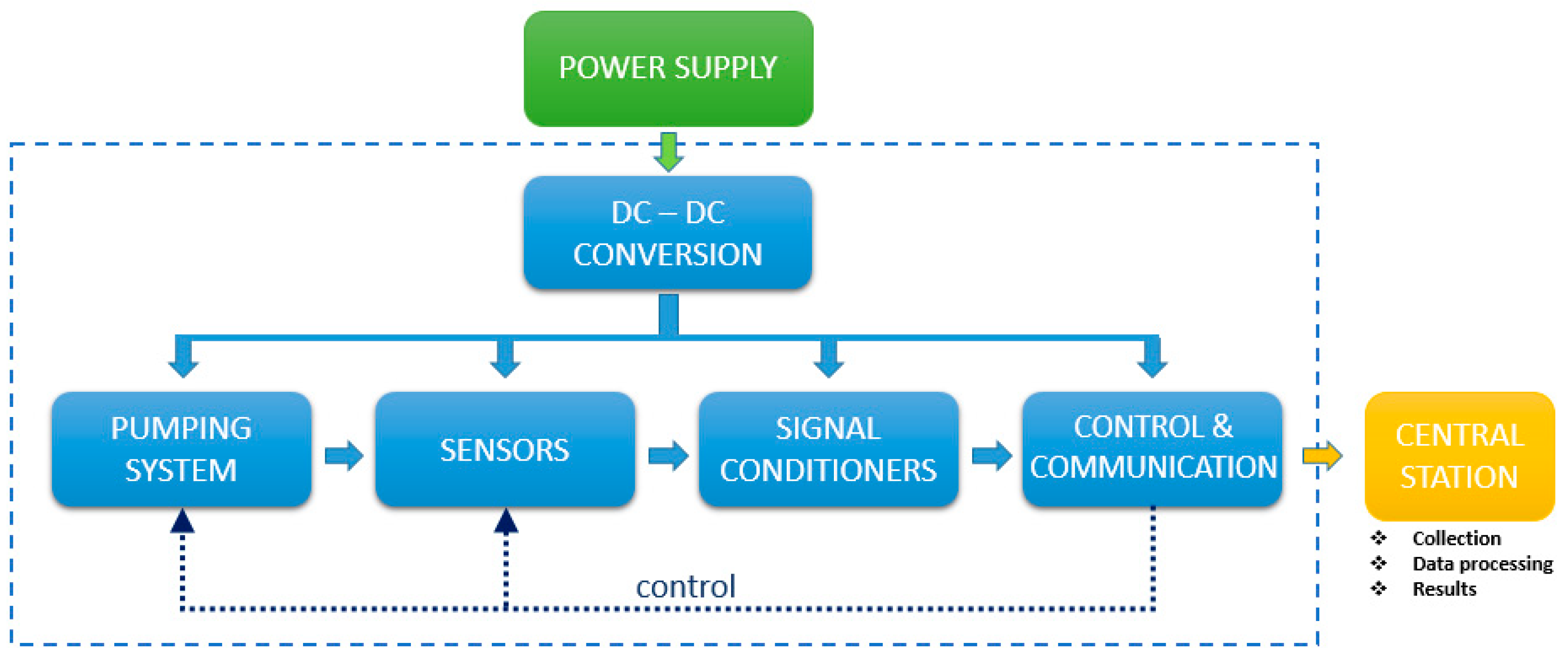
This paper describes the development of a wireless sensor network (WSN) for gas sensors to detect air quality. During the evolution of the project, four different prototypes of the device were developed: prototype version 1 (PV1) [31], prototype version 2 (PV2), prototype version 3 (PV3) [32], and prototype version 4 (PV4). In general, the scheme of the different designs is similar (shown in Figure 1). The corresponding energy source in each case powers the entire device through different voltage converters. Firstly, an optional pumping system carries the gas samples to the sensors cell. These sensors change their electrical resistance in the presence of the different gaseous compounds, which is translated into a voltage change. The signal is conditioned and filtered so that it can be received by the chosen radio frequency (RF) module. This module is responsible for wirelessly sending all the information received to a central station, where the data processing can be performed to obtain the final results in terms of concentration prediction or classification of gas. On the other hand, the RF module is also responsible, in some cases, for controlling the pump system and the sensor heaters (necessary for proper operation of gas sensors).
Throughout the evolution of the system, four different prototypes were designed and developed, depending on the context of the application and also improving on the previous ones. The first version was a homemade prototype created to study the operation of ZigBee communication and gas sensors. The second system incorporated improvements in system autonomy and a greater versatility for using different types of sensors. The third one included changes in communication and data acquisition (incorporating the use of a data cloud), and improved the adaptation of the sensors signals and their stability. Finally, the last system is the most optimized, incorporating solar power and greater autonomy, greater adaptation and control of the sensors, and improvements in the acquisition and processing of data.
2.1. Evolution of Power Supply
2.1.1. Battery Chargers
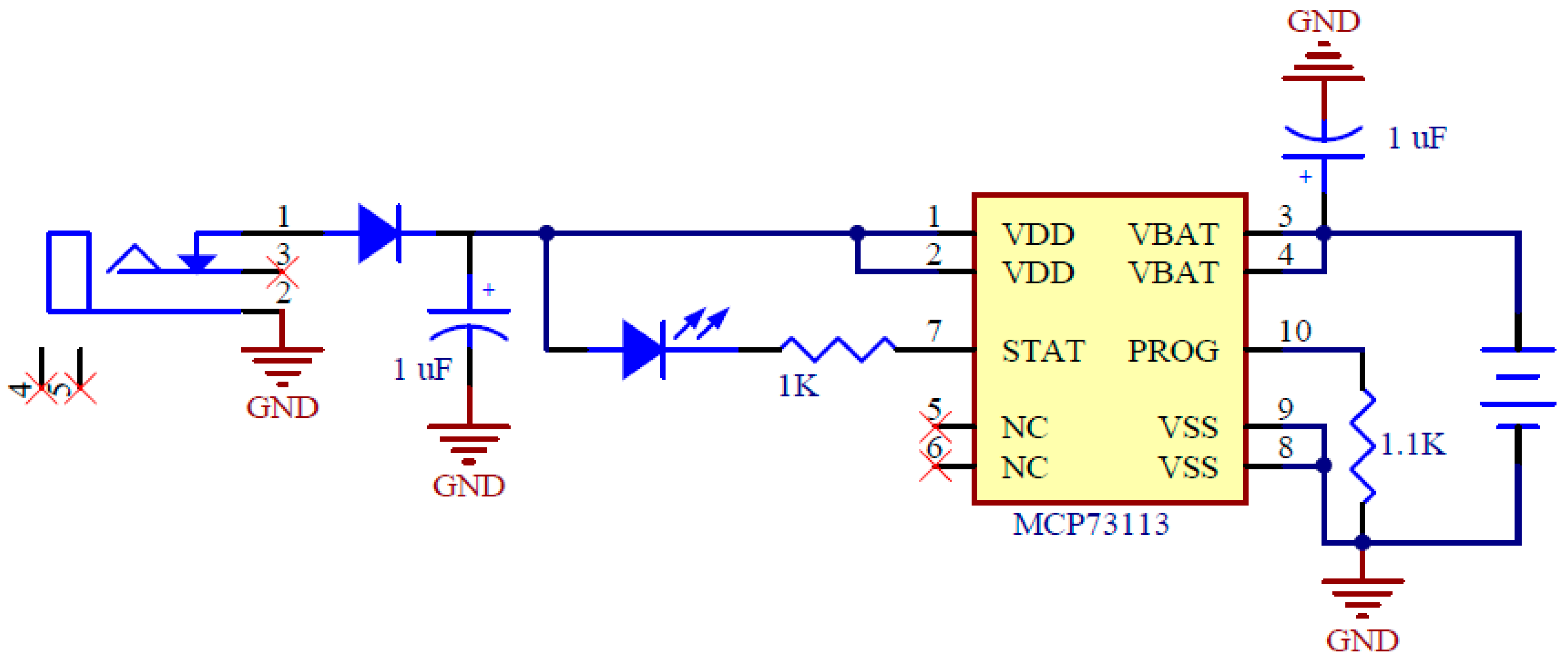
The first prototype (PV1) was powered by a 9-V nickel metal hydride battery with a capacity of 155 mAh that allowed portability. However, an autonomy of more than 1.5 h was not achieved (3.5 h while maintaining the RF module in low-consumption mode in measurements with low sampling frequency, ≤1 sample per hour). For this reason, in PV2 and PV3, a lithium-ion battery of 3.7 V and 1350 mAh was incorporated. In addition, in PV2, a charger circuit was also included to facilitate charging through an external jack connector. The core of this circuit was the MCP73113/4 chip (Microchip, Chandler, AZ, USA), an integrated lithium-ion battery charge management controller with overvoltage protection. In particular, it provides specific charging algorithms for the batteries and, thus, achieves an optimal and safe capacity in the shortest possible charging time. The load current is programmed from the value of an external resistor connected to a 10-pin chip. In this case, a limiting value of 1000 mA was chosen (Figure 2).
This circuit was eliminated in the third prototype because the location where it was going to be used had no external source, thus allowing the optimization of the size of the PCB (Printed Circuit Board).
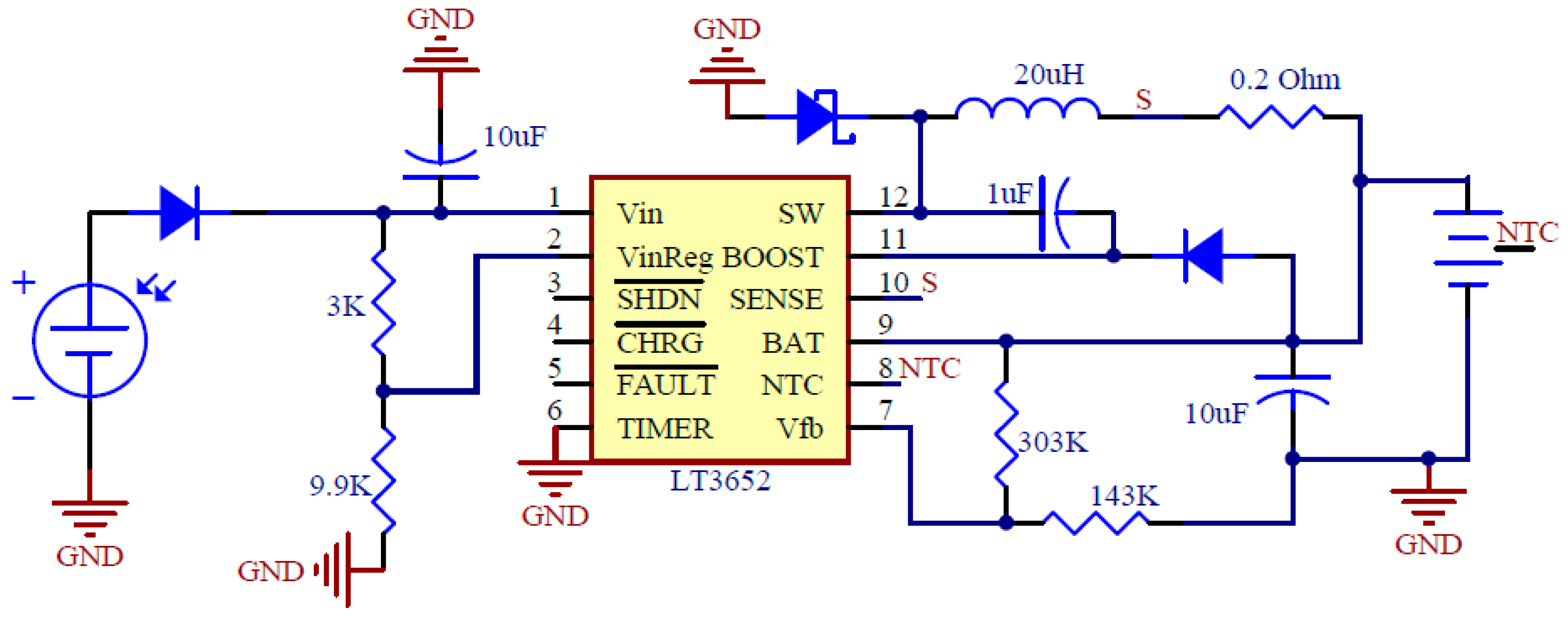
The last and current prototype (PV4) includes a 3.7-V and 2050-mAh battery that, together with a solar panel, greatly improves the autonomy of the system. For this purpose, the LT3652 charger integrated circuit (Linear Technology, Milpitas, CA, USA), optimized for solar panel applications, is used (Figure 3). This circuit keeps the solar panel at the maximum output power and the charging current is modified according to the battery state at each moment. In addition, it has temperature protection and a timer.
2.1.2. Voltage Converters
With respect to the voltage transformation, different converters were used in the different versions of the device. In PV1, linear regulators with up to 250 mA of 3.3 V (for the XBee module) and 5 V (for the sensors) were used. PV2 had an adjustable and disconnectable step-up converter for the sensors, since the battery voltage was changed from 9 V to 3.7 V. This was replaced by two direct current (DC)–DC converters with fixed output voltage (5 V) in PV3 and PV4. This change was due to the high instability in the voltage that distorted the functioning of the sensors. Both converters have different functions: one is used to power the pumping system (pump and electrovalve), while the other allows powering the sensor devices (heating resistor and sensor) more accurately and efficiently.
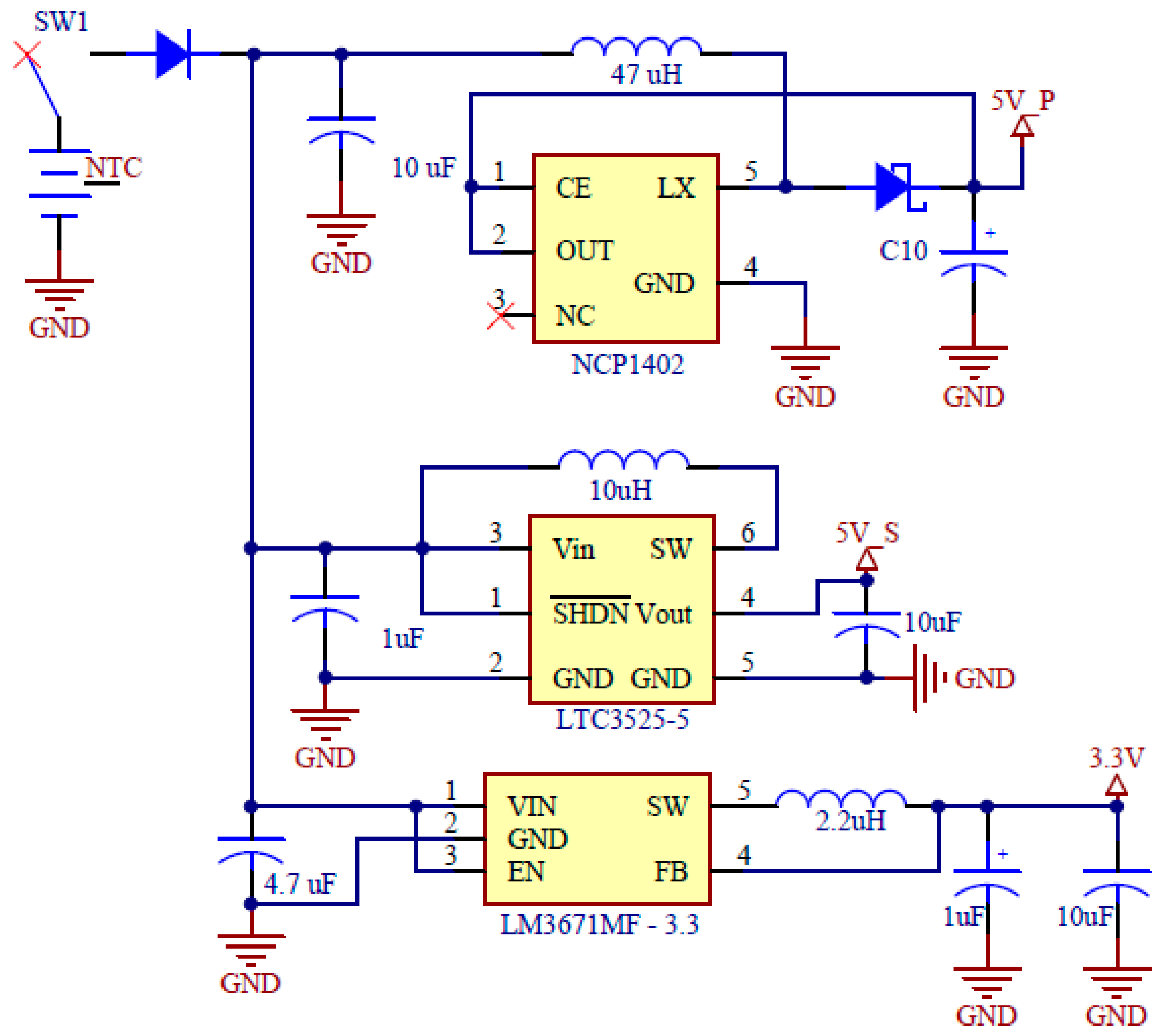
Figure 4 shows the electrical scheme in the case of PV4. It shows that the step-up DC–DC converter NCP1402 (ON Semiconductor, Phoenix, AZ, USA), capable of providing 200 mA, was used to power the pumping system (5V_P); the high efficiency step-up DC–DC converter LTC3525-5 (Linear Technology, Milpitas, CA, USA), capable of supplying 400 mA at the output, was used to power the sensors (5V_S); and the step-down DC–DC converter LM3671MF-3.3 (Texas Instruments, Dallas, TX, USA) was used to power the XBee communication module (3.3 V).
2.2. Sensors and Evolution of Signal Conditioning
2.2.1. Gas Sensors
All sensors used in this work are commercial resistive gas sensors. Specifically, they are semiconductor metal oxide (MOX) sensors whose electrical conductivities are modulated as a result of a reaction between the semiconductor and the gases in the atmosphere. These types of sensors need to be heated in a localized and uniform way or using a pulsed mode between 200 and 450 °C to keep them at an optimum temperature for gas detection [33,34]. It is necessary to carefully control the temperature because the sensitivity of the sensor is strongly dependent on it. Therefore, such sensors include an integrated heating element. The pulsed-temperature operating mode [35] consists of using short heating or cooling pulses from a reference temperature (ambient, high, or intermediate temperature). This mode of operation promotes transient chemical reactions.
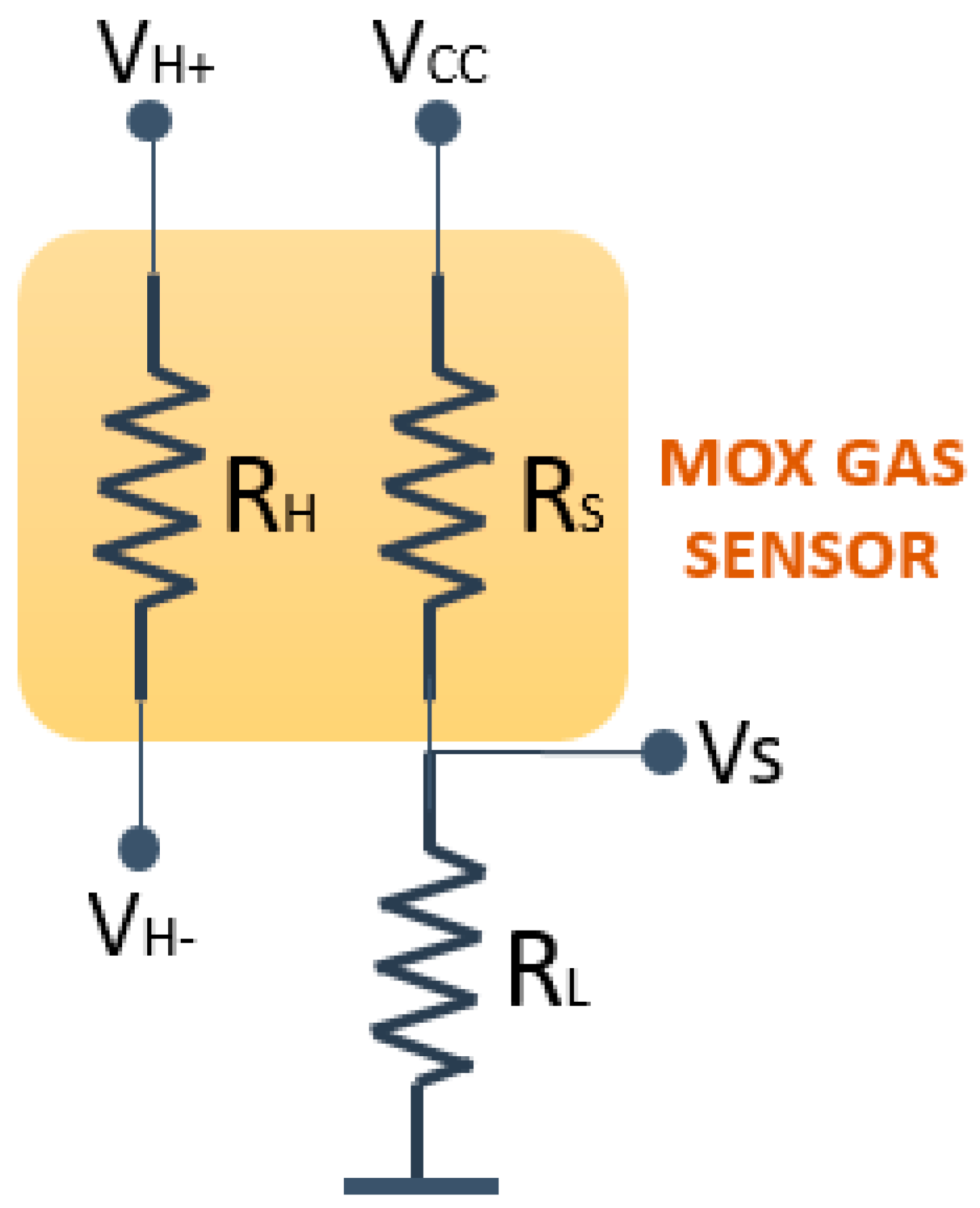
The equivalent circuit for these sensors is composed of heating resistance (RH) and a sensor resistance (RS) components. Figure 5 shows the general circuit recommended by the manufacturers, where a heating voltage (VH) is applied to RH and a supply voltage (VCC) to RS. In addition, a load resistance (RL) is used to obtain an output voltage (VS), which depends on the following equation:
VS = (VCC × RL)/(RS + RL).
2.2.2. Signal Conditioning Circuits
Regarding the conditioning circuit of the sensor signal, PV1 was only composed of the load resistor together with a capacitor to reduce electromagnetic noise and provide low impedance to the analog input of the XBee communication module. In the second and third prototypes, a voltage follower was added to avoid the loading effect. Furthermore, in the second prototype, a variable resistor was used as load resistance (seeking more versatility of the system). However, because it destabilized the system, a fixed resistor was again used in the third version. Finally, the final prototype added the ability to amplify the signal for applications with low-signal sensors.
On the other hand, the power circuits of the heating resistance of the sensors also evolved. In the first device, a voltage of 5 V was directly applied to the heating resistor. Then, a variable resistor was added, since not all the sensors needed the same power for proper operation. In the third version, this variable resistor was replaced by a fixed one (as in the case of the conditioning circuit for the sensor signal), and the heating element activation and deactivation functionality was incorporated using a digital output of the XBee module and a bipolar transistor. Thus, it managed to reduce consumption when sensors were not necessarily working. Finally, PV4 added a heater power control through a PWM (Pulse-Width Modulation) output and a MOSFET transistor, thereby achieving the possibility of modifying the operating temperatures of the gas sensors and of using the pulsed-temperature operating mode.
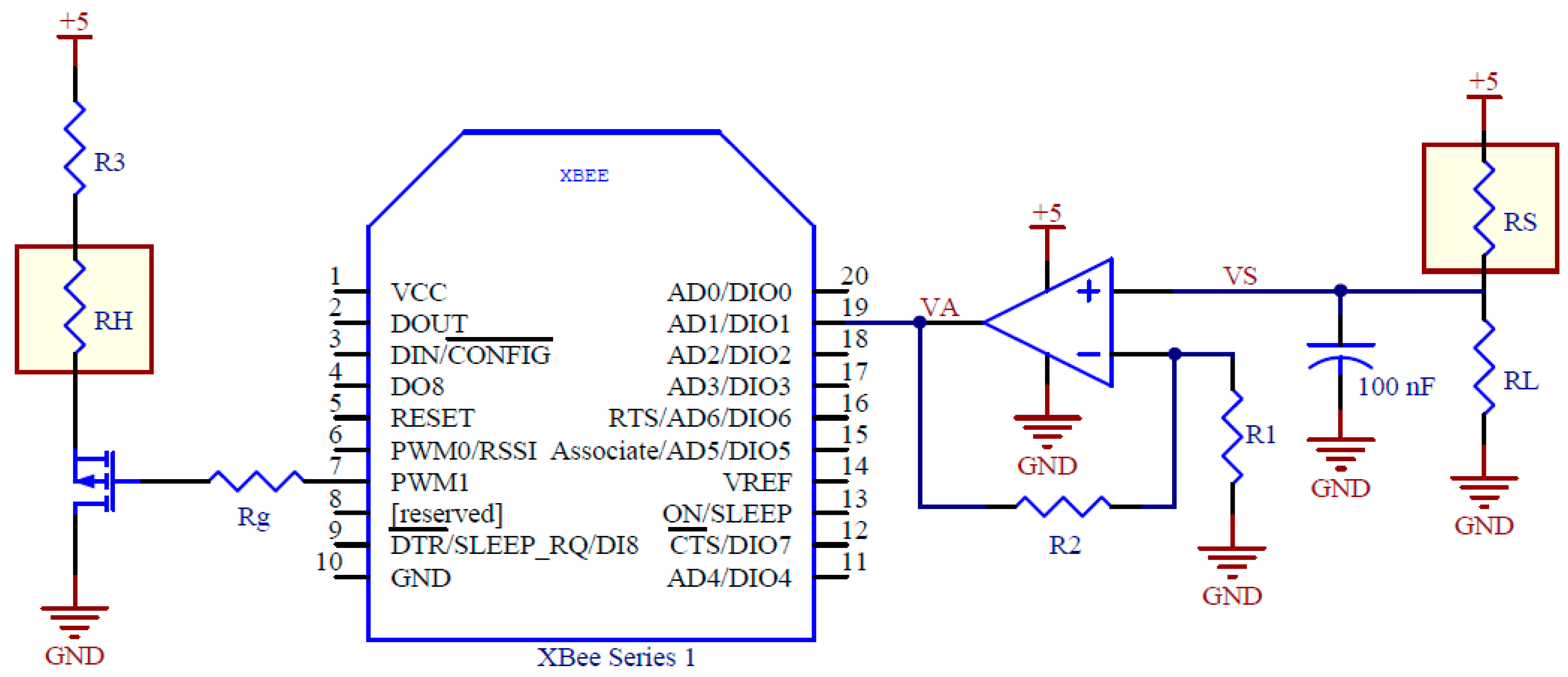
Figure 6 shows the final electrical diagram of the sensor signal conditioning and of the heating power control in PV4. RH corresponds to the heating resistance, R3 is the resistor placed in series to limit the maximum current in RH, Rg is the gate resistor, VS is the output voltage of the gas sensor, R2 and R1 are the resistors corresponding to the amplification circuit of the signal, RS is the resistance of the sensor, RL the load resistor corresponding to the sensor, and VA is the output voltage of the amplifier stage, and the input to the analog/digital converter of the XBee module.
According to this, the input voltage in the XBee module is defined by the following equation (corresponding to the non-inverting amplifier):
VA = (1 + R2/R1) × VS.
2.3. Sampling System
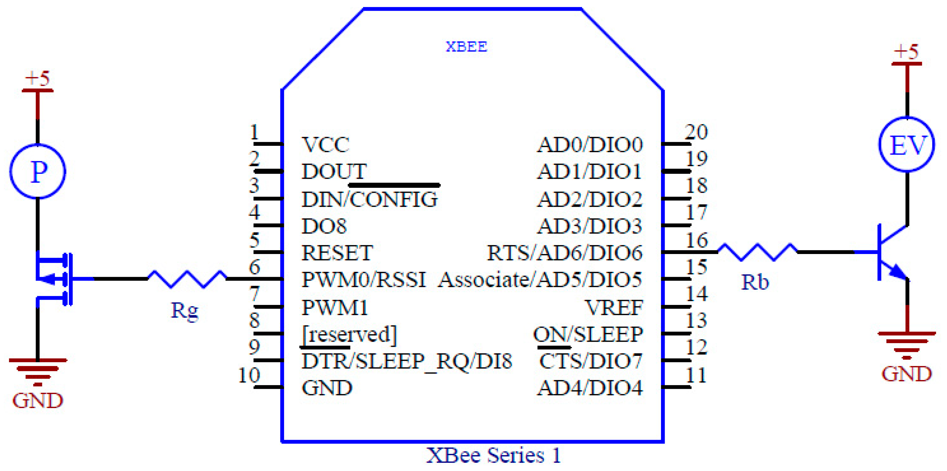
The sampling system takes a representative sample of the air to be analyzed, which is carried to the sensor cell. From the second prototype onward, the sampling system included a pump and an electrovalve in the sensor nodes in order to be connected to the system and to control the headspace from liquid samples for doing several measurements in the laboratory. In this way, it was possible to switch between a reference gas and a target gas and lead it to the sensor cell. For this purpose, a PWM output was used for adjusting pump speed, and a digital output was used for controlling the electrovalve state. In the first case, a MOSFET transistor and a gate resistor were used, while, in the second case, a bipolar transistor and the corresponding base resistor were used (Figure 7).
2.4. RF Module (XBee) and Evolution of Wireless Communication
The wireless communication devices used were the XBee radio frequency modules [36], which work in the 2.4-GHz band and with the IEEE 802.15.4 communication protocol. These are developed by Digi International (Minnetonka, MN, USA), and allow the creation of ZigBee networks (oriented to systems of low data transfer and consumption). They also incorporate a microcontroller (M9S08GT60, Freescale, Austin, TX, USA) to control all other peripherals. The module has seven ports configurable as digital inputs/outputs or analog inputs, along with two more digital inputs and outputs, and two PWM outputs.
In the first and second prototypes developed in this work (PV1 and PV2), the communication network was formed by the sensor nodes and a coordinator node responsible for receiving information from all others. To implement this coordinator node, a commercial interface card was used to communicate the XBee module with a computer via universal serial bus (USB). For receiving data and for configuration and monitoring of the entire network, an application was developed in LabVIEW. Then, data were stored on the computer for further processing.
In PV3, as before, the network consisted of some sensor nodes responsible for receiving the information and sending it, following the ZigBee protocol. However, in this case, the network coordinator node was the gateway “ConnectPort X4” (Digi, Minnetonka, MN, USA). It was connected to the internet via ethernet, and was responsible for submitting the information collected by the sensor nodes to the commercial cloud “Device Cloud” from Digi, where it is stored in XML format.
For programming, the “ConnectPort X” gateways offer a built-in Python® engine, providing a powerful open-source software tool to develop custom applications that run on the gateway. In this study, several Python® applications were developed for controlling the network. Among them, two stand out, which allow the information received by the nodes to be separated and pre-processed and then sent and stored in the data cloud. The difference between these two applications is that one was designed for laboratory measurements and, therefore, controls the pump and the electrovalve for switching between a reference gas and the target gas. The other application was designed for field applications, with an uncontrolled gas inlet to the sensor cell.
Finally, in the latest version, a self-developed data cloud was created in order to receive data from the sensor network and to provide storage services, classification, and requests.
2.5. Summary of Evolution of Prototypes
Table 1 shows the different main characteristics of each of the developed versions of the wireless sensor network for air quality measurements. It specifies the different sizes, the maximum and minimum consumption, and the autonomy, whether the gas sensors were integrated within the node or were connectable from an external PCB, as well as the tools used to receive, store, and process the collected data by the sensor nodes, whether they included a connection and control capacity for the pumping system, and the main features of improvement with respect to the previous version. The evolution was geared toward greater autonomy, smaller size, and greater flexibility and versatility.
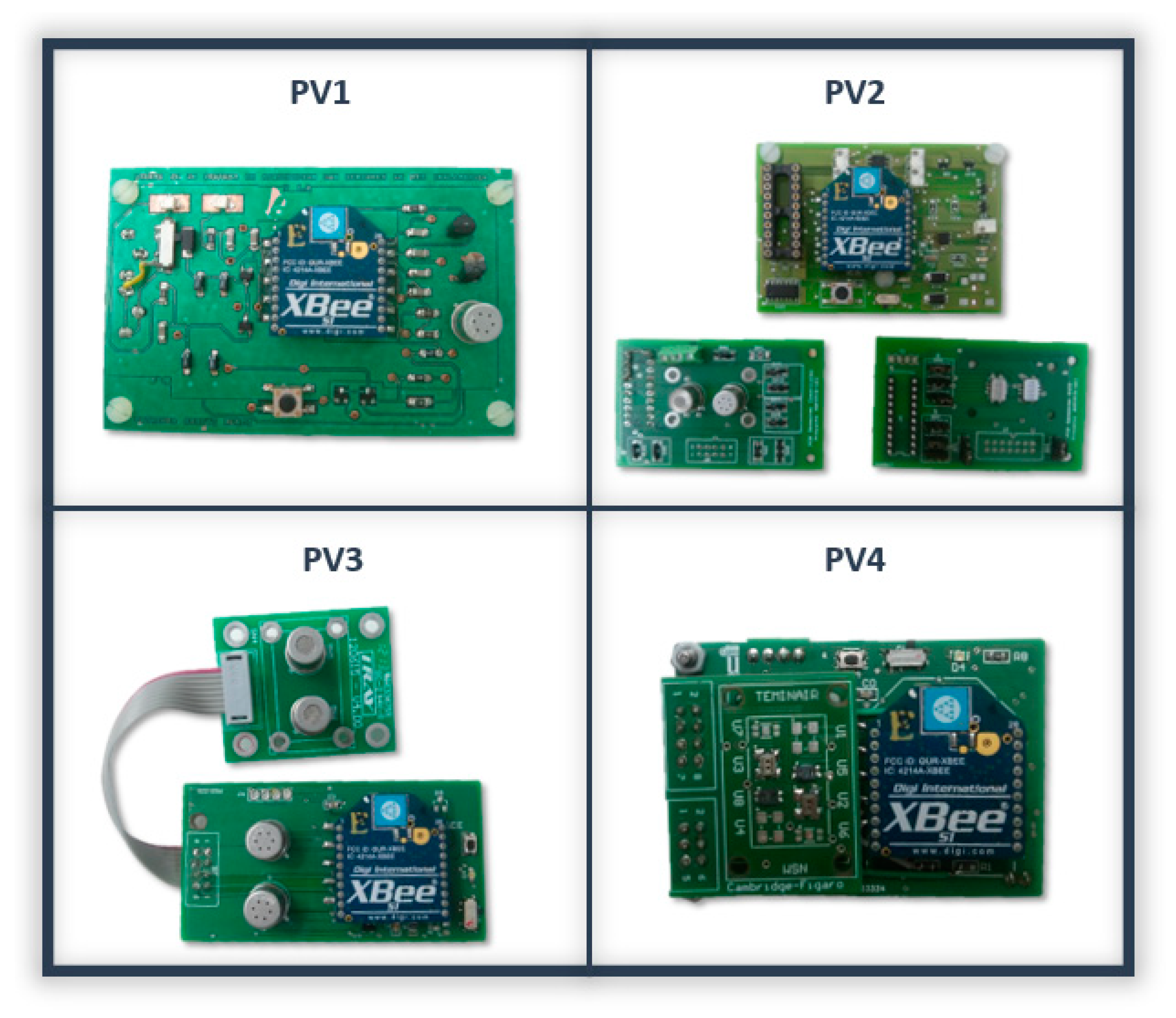
Pictures of the evolution of the wireless gas sensor nodes described in this paper are presented in Figure 8.
2.6. Data Processing
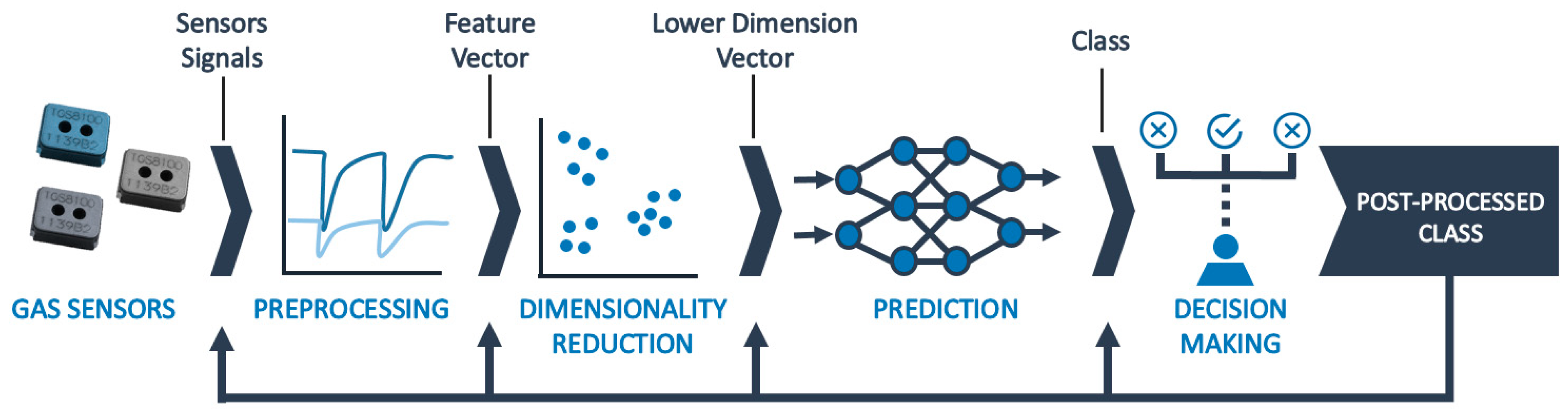
For proper device operation, it is necessary to use data processing techniques and artificial intelligence algorithms. In this process, four stages are typically performed (Figure 9): preprocessing, reduction of the number of variables, prediction, and decision-making.
Firstly, pre-processing techniques are applied to the collected data. In this case, this stage is performed in real time on the gateway. One of the existing feature extraction algorithms in the literature according to Gutierrez-Osuna [30] was used, namely the relative resistance algorithm (RR). Following this algorithm, the characteristic value of each measurement is defined by the following equation:
where RV is the resistance value in exposure to the reference compound (air) and RN is the resistance value in exposure to the target compound, both in steady-state situations.
RR = RV/RN,
To reduce the size of the extracted data, the principal component analysis (PCA) [37] technique was used. This technique reduces the dataset, losing the least amount of information possible. It employs linear combinations of the original variables resulting in linearly independent variables. This phase and the following phase are performed in the cloud system.
Next, the prediction phase is carried out. At this stage, regression techniques can be applied to quantify concentrations, while classification techniques can be applied to discriminate contaminating compounds, or clustering techniques can be applied to group similar responses. In the results shown in this article, classification tasks were applied. To this end, probabilistic neural networks (PNN) were used, also called radial basis networks due to the use of a neuron activation radial basis function (RBF) [38]. These networks are made up of four layers. The input layer corresponds to the PCA components used. The next one is the pattern layer, with a number of neurons equal to the training vectors, grouped by classes, where the distance between the input layer vector and each element of the training set was evaluated. The third layer, i.e., the summation layer, contains a neuron for each class and adds the outputs of the pattern neurons belonging to the same class. Lastly, the output layer is a “limiter” that seeks the maximum value of the sum layer. Then, the highest value is selected and set to 1 as a result, while the other outputs are set to 0.
Finally, to determine the validity of the system, predictions of known values were made to compare the estimate values with the real results. Leave-one-out cross-validation (LOOCV) was used to determine the performance of the trained model in this case. This validation technique proposes to perform as many iterations as samples present in the dataset.
3. Results and Discussion
3.1. Measurement Set-Up
The same measurements were made for each of the versions of the designed wireless networks, except in the case of the PV1, which was developed in order to make first contact with the technology used, and only had one gas sensor (TGS2600, Figaro, Japan).
The array of sensors used in each prototype for the following measurements are as follows:
- 2 × TGS2600 (Figaro, Japan) and 2 × TGS2620 (Figaro, Japan) in PV2 and PV3.
- 2 × TGS8100 (Figaro, Japan), 1 × CCS801, and 1 × CCS803 (ams, UK) in PV4.
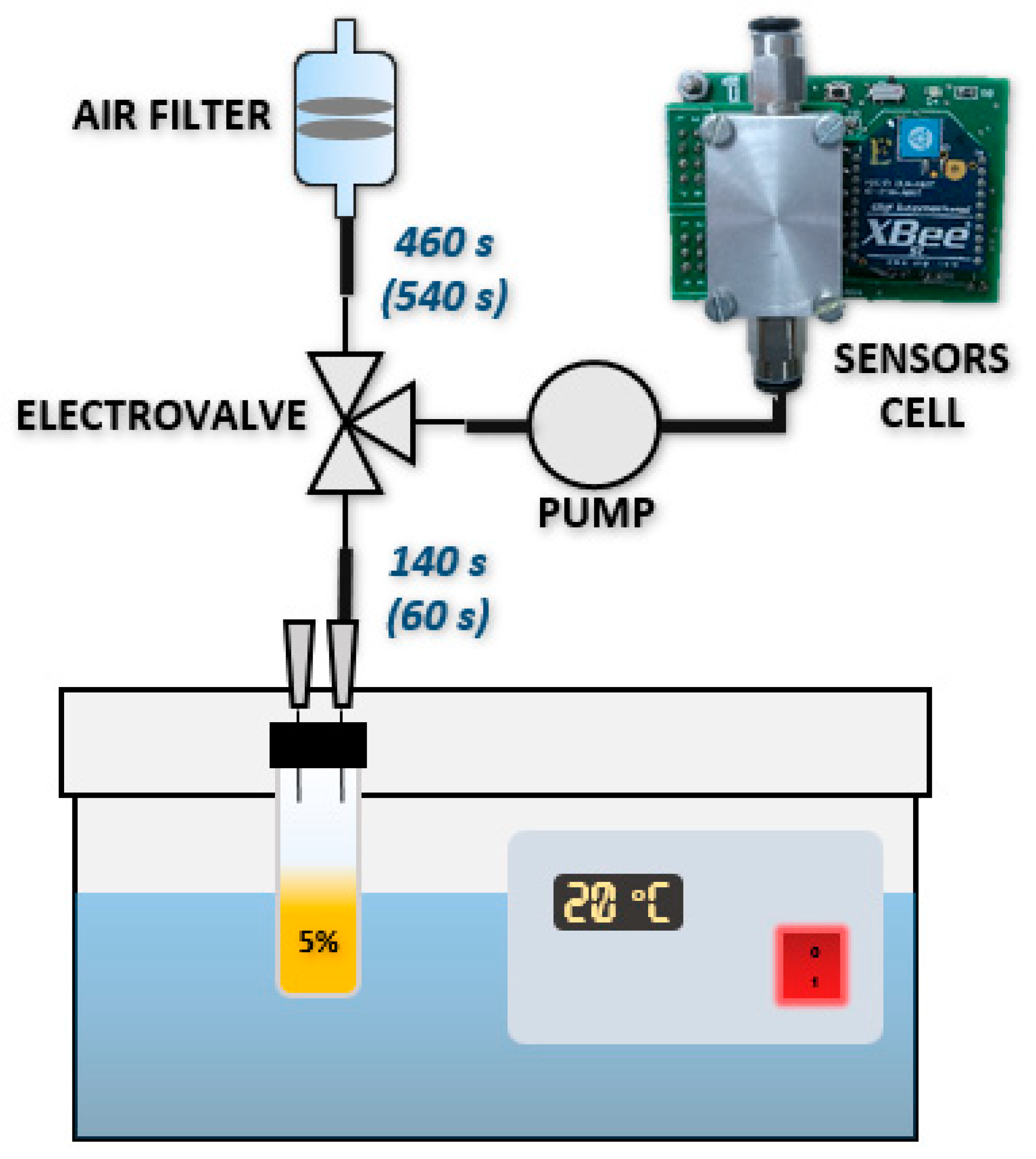
These tests attempted to analyze the ability of devices to discriminate the BTEX (benzene, toluene, ethylbenzene, and xylene) volatile organic compounds dissolved in water. For this purpose, the static head space technique was used in 22-mL vials. Samples of 10 mL were prepared at a 5% concentration of each compound. Then, the headspace was drawn into the sensor cell using a pump. The vials were kept at 20 °C. Each measurement cycle lasted 10 min: 140 s for the passage of the target compound to the sensor cell, and 460 s for the flow of the reference gas (in this case, clean air). In the measurements made with the final prototype, these times were updated to 60 s (target) and 540 s (reference) to ensure the signal stabilization in the reference gas phase. Figure 10 shows a diagram of the measurement process.
More than 15 measurements were taken for each one of the BTEX compounds and distilled water (in order to have a reference of absence of simulated contaminants in the environment).
3.2. Results
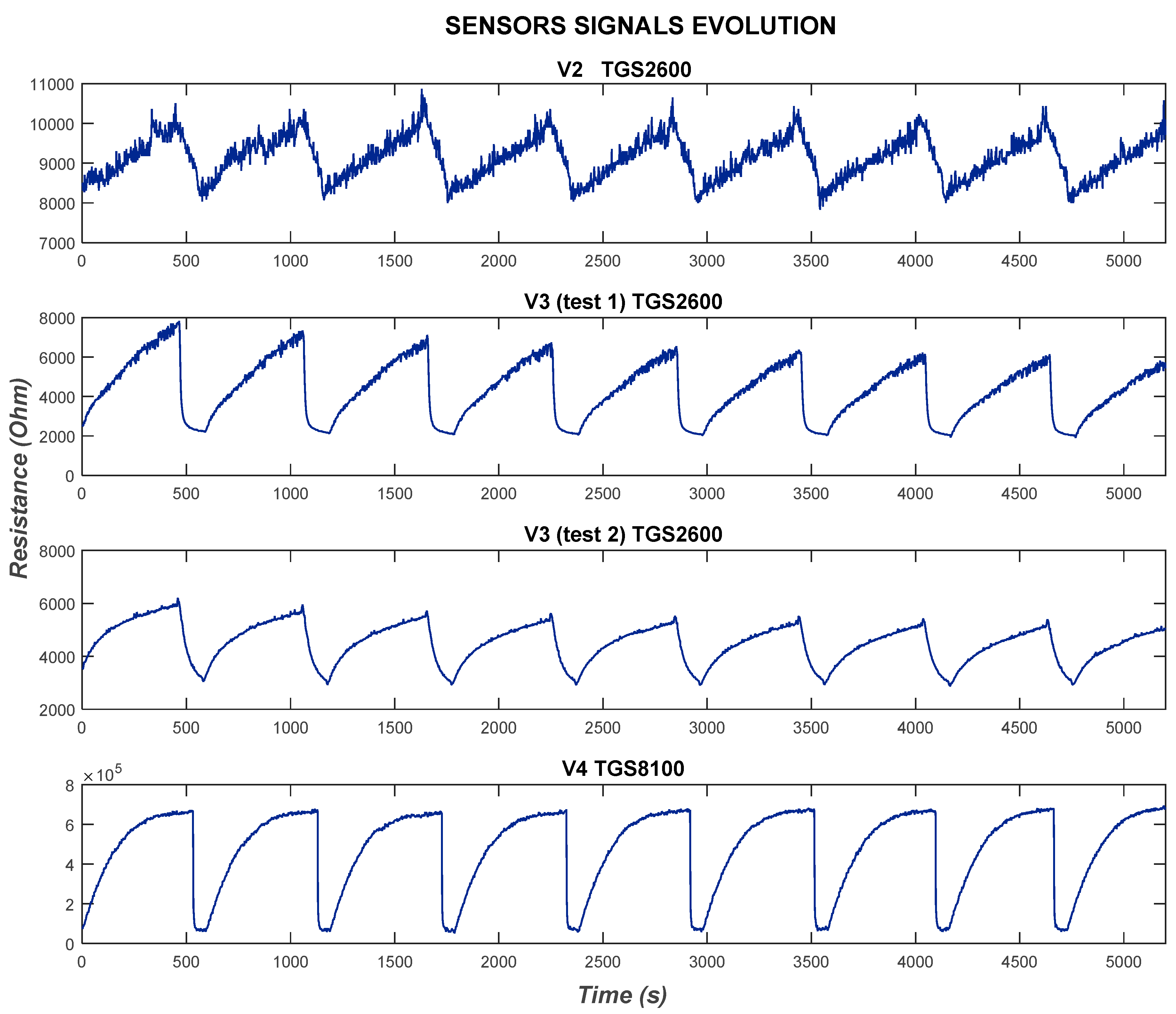
The signals obtained from one of the sensors of each of the four sets of measurements are shown in Figure 11. The selected signals correspond to eight measurement cycles of xylene in each case. One of the sensors (model TGS2600) was selected for PV2 and PV3. Because PV4 did not use this sensor model, the signal of sensor model TGS8100, from the same manufacturer, was selected. The evolution shows the improvement achieved in each version due to changes in the power and conditioning circuits, pump power, and timing optimization. Thus, between the first two sets of measurements, noise reduction was achieved thanks to the changes introduced in the conditioning and power circuits of the sensors, and changes in the heater temperature. Then, between the second and third package (made with the same version of the device, PV3), further noise reduction and a greater stabilization of the signal were achieved by decreasing the flow rate of the sample (by controlling the power of the pump). Finally, between the last two sets of measurements, in addition to the changes introduced in the adaptation and control circuitry, a faster response was achieved due to the use of a sensor of smaller size and consumption.
Once all the data from the measurements were collected, data processing was performed. In the case of PV2, the preprocessing phase was done manually through the Matlab software. However, in the third and fourth versions, this process was performed automatically (while measurements were made) by the program developed in Python that ran on the gateway. As explained above, this preprocessing phase used the relative resistance algorithm. It extracted the value of the ratio between the resistance value of the baseline and the resistance value during exposure to the target compound. In this way, it was possible to extract the main information, while considerably reducing the size of the data.
In all cases, the first two measures were discarded, since the systems were not yet stabilized and the conditions were not the same. Therefore, 13 measurements of each compound were used for data processing.
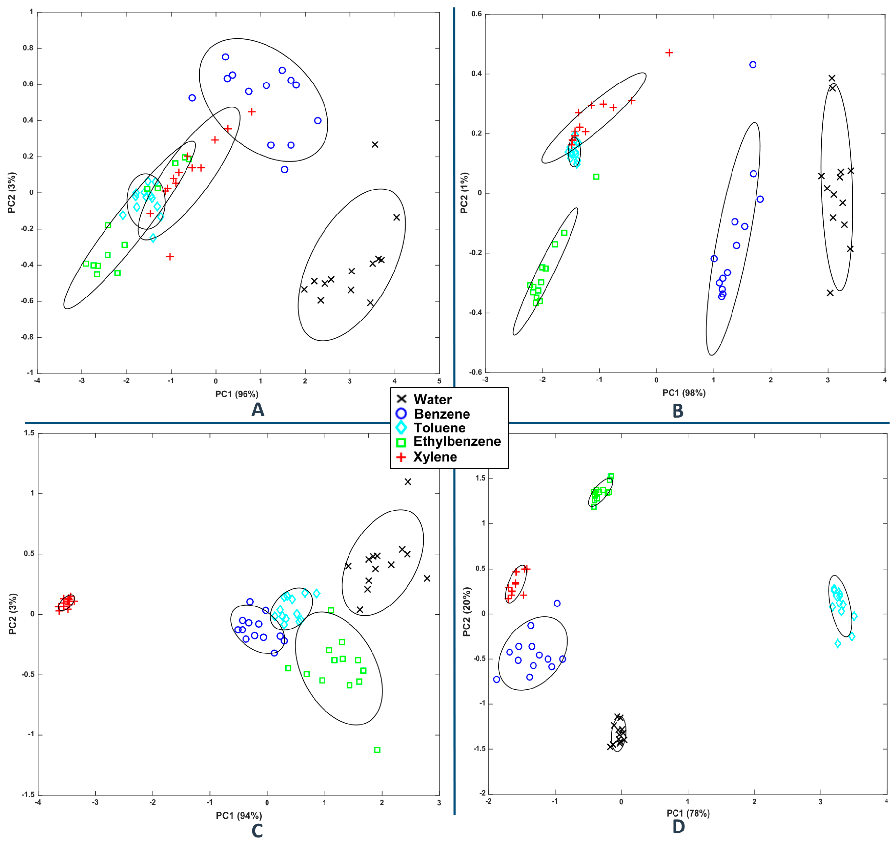
Then, an analysis of the main component (PCA) was carried out for a graphical representation of the measurements. Figure 12A shows the first two principal components of the measurements made with PV2. A high overlap can be observed between some compounds such as toluene, benzene, and xylene. In addition, short-term drift and dispersion effects appear, resulting from high noise in the measurements and non-stable temperature of the gas sensor heaters. The PCA of the same measurements made with PV3 is presented in Figure 12B. It shows that the clusters are further apart than in the previous case, although there is still overlap between those of toluene and xylene. Furthermore, a high drift effect is still present, possibly due to depletion of the sample. A similar test was repeated using lower pump power in the extraction phase of the sample (test 2). Moreover, the preprocessing program was improved, achieving greater accuracy of obtaining the characteristic value of each measurement. In Figure 12C, it can be observed that the PCA plot improved significantly, managing to reduce the drift effect and the overlaps between zones (only a small overlap between the areas of benzene and toluene, although they are generally very close to each other). Finally, Figure 12D shows the first two principal components of the values of the measurements made with the latest version of the device (PV4), where it can be observed that different areas concerning each compound are clearly separated and non-dispersed.
Next, PNN was used in order to discriminate the compounds. Then, the LOOCV validation technique was used to study the classification capacity in each case. The results of each of the four studied cases are presented in Table 2, which contains the confusion matrix obtained, allowing us to observe the system performance. The matrix columns represent the predicted class, and the rows represent the real class. As a result, the main diagonal contains correct predictions, while values outside it correspond to erroneous ones. Red data represent the matrix corresponding to the results of PV2. Blue data correspond to the first test performed with PV3 (without preprocessing and pump power correction), while green data correspond to the second test (with correction) of PV3. Finally, the black columns refer to the data resulting from PV4. The resulting success rates were 80%, 93.84%, 96.82%, and 100% for the four datasets, respectively.
4. Conclusions
In this paper, a wireless gas sensor network focusing on the study of air quality was presented. For this purpose, the electronic evolution of the designed sensor nodes was described, until a node of low cost, low consumption, and small size was obtained. Up to four gas microsensors can be connected to the nodes. In addition, they incorporate a control and RF module with ZigBee protocol that allows communication with a central node. This, in turn, is responsible for collecting and storing the data, controlling some aspects of the sensor nodes, and, in the most advanced prototype, preprocessing the data and uploading it to a data cloud.
The system was designed to be used in pollutant detection applications and air quality control in large areas. In order to verify the proper operation and discrimination capacity of the system, discrimination tests of BTEX volatile organic compounds were carried out. These tests also allowed studying the evolution of system operation. As a result, the signals were observed to improve significantly, and the discrimination success rates increased from 80% (PV1) to 100% (PV4).
Author Contributions
P.A. designed the hardware and performed the measurements; J.I.S. and J.L. designed the control architecture and the experiments. All authors wrote the article.
Funding
The authors want to thank the Spanish Ministry of Economy and Competitiveness and Junta de Extremadura for supporting the TEC2013-48147-C6-5-R and IB16048 projects.
Acknowledgments
The authors want to thank José Luis Herrero for help with the cloud system, and Pablo Carmona, Juan Álvaro Fernandez, and Carlos Sánchez for help with the data processing methods.
Conflicts of Interest
The authors declare no conflict of interest.
References
- WHO. The Cost of a Polluted Environment: 1.7 Million Child Deaths a Year, Says WHO; World Health Organization: Geneva, Switzerland, 2017. [Google Scholar]
- McCarthy, N. Air Pollution Contributed to More Than 6 Million Deaths in 2016; Forbes: New York, NY, USA, 2018. [Google Scholar]
- WHO. Esposure to Benzene: A Major Public Health Concern; World Health Organization: Geneva, Switzerland, 2010. [Google Scholar]
- Lung, C.; Jones, R.; Zellweger, C.; Karppinen, A.; Penza, M.; Dye, T.; Hüglin, C.; Ning, Z.; Leigh, R.; Hagan, D.; et al. Low-Cost Sensors for the Measurement of Atmospheric Composition: Overview of Topic and Future Applications (WMO); Lewis, A.C., Von Schneidemesser, E., Peltier, R., Eds.; World Meteorological Organization: Geneva, Switzerland, 2018; ISBN 9789263112156. [Google Scholar]
- Yick, J.; Mukherjee, B.; Ghosal, D. Wireless sensor network survey. Comput. Netw. 2008, 52, 2292–2330. [Google Scholar] [CrossRef]
- Rawat, P.; Singh, K.D.; Chaouchi, H.; Bonnin, J.M. Wireless sensor networks: A survey on recent developments and potential synergies. J. Supercomput. 2014, 68, 1–48. [Google Scholar] [CrossRef]
- Yi, W.Y.; Lo, K.M.; Mak, T.; Leung, K.S.; Leung, Y.; Meng, M.L. A Survey of Wireless Sensor Network Based Air Pollution Monitoring Systems. Sensors 2015, 15, 31392–31427. [Google Scholar] [CrossRef] [PubMed] [Green Version]
- Othman, M.F.; Shazali, K. Wireless Sensor Network Applications: A Study in Environment Monitoring System. Procedia Eng. 2012, 41, 1204–1210. [Google Scholar] [CrossRef]
- Baranov, A.; Spirjakin, D.; Akbari, S.; Somov, A. Optimization of power consumption for gas sensor nodes: A survey. Sens. Actuators A Phys. 2015, 233, 279–289. [Google Scholar] [CrossRef]
- Shaikh, F.K.; Zeadally, S. Energy harvesting in wireless sensor networks: A comprehensive review. Renew. Sustain. Energy Rev. 2016, 55, 1041–1054. [Google Scholar] [CrossRef]
- Farahani, S. Chapter 3—ZigBee and IEEE 802.15.4 Protocol Layers. In ZigBee Wireless Networks and Transceivers; Elsevier: Amsterdam, The Netherlands, 2008; pp. 33–135. [Google Scholar]
- De Guglielmo, D.; Brienza, S.; Anastasi, G. IEEE 802.15.4e: A survey. Comput. Commun. 2016, 88, 1–24. [Google Scholar] [CrossRef]
- Baronti, P.; Pillai, P.; Chook, V.W.C.; Chessa, S.; Gotta, A.; Hu, Y.F. Wireless sensor networks: A survey on the state of the art and the 802.15.4 and ZigBee standards. Comput. Commun. 2007, 30, 1655–1695. [Google Scholar] [CrossRef] [Green Version]
- Huang, Y.; Hu, L.; Yang, D.; Liu, H. Air-Sense: Indoor environment monitoring evaluation system based on ZigBee network. IOP Conf. Ser. Earth Environ. Sci. 2017, 81, 12208. [Google Scholar] [CrossRef]
- Kasar, A.R.; Khemnar, D.S.; Tembhurnikar, N.P. WSN Based Air Pollution Monitoring System. Int. J. Sci. Eng. Appl. 2013, 2, 2319–7560. [Google Scholar] [CrossRef]
- Yang, C.-T.; Chen, S.-T.; Den, W.; Wang, Y.-T.; Kristiani, E. Implementation of an Intelligent Indoor Environmental Monitoring and management system in cloud. Future Gener. Comput. Syst. 2018. [Google Scholar] [CrossRef]
- Botta, A.; de Donato, W.; Persico, V.; Pescapé, A. Integration of Cloud computing and Internet of Things: A survey. Future Gener. Comput. Syst. 2016, 56, 684–700. [Google Scholar] [CrossRef]
- Herrero, J.L.; Lozano, J.; Santos, J.P.; Suárez, J.I. On-line classification of pollutants in water using wireless portable electronic noses. Chemosphere 2016, 152, 107–116. [Google Scholar] [CrossRef] [PubMed]
- Li, W.; Kara, S. Methodology for Monitoring Manufacturing Environment by Using Wireless Sensor Networks (WSN) and the Internet of Things (IoT). Procedia CIRP 2017, 61, 323–328. [Google Scholar] [CrossRef]
- Kumar, P.M.; Lokesh, S.; Varatharajan, R.; Gokulnath, C.; Parthasarathy, P. Cloud and IoT based disease prediction and diagnosis system for healthcare using Fuzzy neural classifier. Future Gener. Comput. Syst. 2018. [Google Scholar] [CrossRef]
- Aleixandre, M.; Gerboles, M. Review of small commercial sensors for indicative monitoring of ambient gas. Chem. Eng. Trans. 2012, 30, 169–174. [Google Scholar] [CrossRef]
- Fine, G.F.; Cavanagh, L.M.; Afonja, A.; Binions, R. Metal oxide semi-conductor gas sensors in environmental monitoring. Sensors 2010, 10, 5469–5502. [Google Scholar] [CrossRef] [PubMed]
- Peterson, P.J.D.; Aujla, A.; Grant, K.H.; Brundle, A.G.; Thompson, M.R.; Vande Hey, J.; Leigh, R.J. Practical use of metal oxide semiconductor gas sensors for measuring nitrogen dioxide and ozone in urban environments. Sensors 2017, 17, 1653. [Google Scholar] [CrossRef] [PubMed]
- Kubinec, R.; Adamuščin, J.; Jurdáková, H.; Foltin, M.; Ostrovský, I.; Kraus, A.; Soják, L. Gas chromatographic determination of benzene, toluene, ethylbenzene and xylenes using flame ionization detector in water samples with direct aqueous injection up to 250 μL. J. Chromatogr. A 2005, 1084, 90–94. [Google Scholar] [CrossRef] [PubMed]
- Hazrati, S.; Rostami, R.; Fazlzadeh, M. BTEX in indoor air of waterpipe cafés: Levels and factors influencing their concentrations. Sci. Total Environ. 2015, 524–525, 347–353. [Google Scholar] [CrossRef] [PubMed]
- Niri, V.H.; Mathers, J.B.; Musteata, M.F.; Lem, S.; Pawliszyn, J. Monitoring BTEX and aldehydes in car exhaust from a gasoline engine during the use of different chemical cleaners by solid phase microextraction-gas chromatography. Water Air Soil Pollut. 2009, 204, 205–213. [Google Scholar] [CrossRef]
- Zali, S.; Jalali, F.; Es-haghi, A.; Shamsipur, M. New nanostructure of polydimethylsiloxane coating as a solid-phase microextraction fiber: Application to analysis of BTEX in aquatic environmental samples. J. Chromatogr. B 2016, 1033–1034, 287–295. [Google Scholar] [CrossRef] [PubMed]
- Allouch, A.; Le Calvé, S.; Serra, C.A. Portable, miniature, fast and high sensitive real-time analyzers: BTEX detection. Sens. Actuators B Chem. 2013, 182, 446–452. [Google Scholar] [CrossRef]
- Marco, S.; Gutiérrez-Gálvez, A. Signal and Data Processing for Machine Olfaction and Chemical Sensing: A Review. IEEE Sens. J. 2012, 12, 3189–3214. [Google Scholar] [CrossRef]
- Gutierrez-Osuna, R. Pattern analysis for machine olfaction: A review. IEEE Sens. J. 2002, 2, 189–202. [Google Scholar] [CrossRef]
- Lozano, J.; Suárez, J.I.; Arroyo, P.; Ordiales, J.M.; Álvarez, F. Wireless sensor network for indoor air quality monitoring. Chem. Eng. Trans. 2012, 30, 319–324. [Google Scholar] [CrossRef]
- Arroyo, P.; Lozano, J.; Suárez, J.I.; Herrero, J.L.; Carmona, P. Wireless sensor network for indoor air quality monitoring and Control. Chem. Eng. Trans. 2016, 54, 217–222. [Google Scholar] [CrossRef]
- Kohl, D. Fundamentals and Recent Developments of Homogeneous Semiconducting Sensors. In Sensors and Sensory Systems for an Electronic Nose; Gardner, J.W., Bartlett, P.N., Eds.; Springer: Dordrecht, The Netherlands, 1992; pp. 53–76. [Google Scholar]
- Moseley, P.T.; Stoneham, A.M.; Williams, D.E. Oxide semiconductors: Patterns of gas response behaviour according to materials type. In Techniques and Mechanisms in Gas Sensing; Moseley, P.T., Norris, J., Williams, D.E., Eds.; Adam Hilger: Bristol, UK, 1991; pp. 108–138. [Google Scholar]
- Presmanes, L.; Thimont, Y.; El Younsi, I.; Chapelle, A.; Blanc, F.; Talhi, C.; Bonningue, C.; Barnabé, A.; Menini, P.; Tailhades, P. Integration of P-Cuo thin sputtered layers onto microsensor platforms for gas sensing. Sensors 2017, 17, 1409. [Google Scholar] [CrossRef] [PubMed]
- Eady, F. Maxstream/XBee. In Hands-On ZigBee; Newnes, Ed.; Elsevier: Amsterdam, The Netherlands, 2007; pp. 131–152. [Google Scholar]
- Esbensen, K.H.; Geladi, P. Principal Component Analysis: Concept, Geometrical Interpretation, Mathematical Background, Algorithms, History, Practice. Compr. Chemom. 2009, 211–226. [Google Scholar] [CrossRef]
- Specht, D.F. Probabilistic neural networks. Neural Netw. 1990, 3, 109–118. [Google Scholar] [CrossRef]
Figure 1.
Block diagram of each node of the WSN.

Figure 2.
Electrical diagram of battery charging system corresponding to prototype version 2 (PV2).

Figure 3.
Electrical diagram of battery charging system from solar panels corresponding to PV4.

Figure 4.
Electrical diagram of voltage conversion corresponding to PV4.

Figure 5.
Equivalent circuit for MOX sensors.

Figure 6.
Electrical diagram of the sensor signal conditioning circuits and of the control of the heating power in PV4.
Figure 6.
Electrical diagram of the sensor signal conditioning circuits and of the control of the heating power in PV4.

Figure 7.
Electrical diagram of the activation circuits of the pump and the electrovalve (PV2, PV3, and PV4).
Figure 7.
Electrical diagram of the activation circuits of the pump and the electrovalve (PV2, PV3, and PV4).

Figure 8.
Real images of the prototypes developed.

Figure 9.
Data processing block diagram.

Figure 10.
Measurements set-up scheme.

Figure 11.
Evolution of sensor signals (resistance versus time), corresponding to the eight xylene measurements.
Figure 11.
Evolution of sensor signals (resistance versus time), corresponding to the eight xylene measurements.

Figure 12.
Principal component analysis (PCA) plot for benzene, toluene, ethylbenzene, and xylene (BTEX) compounds of the different datasets: (A) PV2; (B) PV3 (test 1); (C) PV3 (test 2); (D) PV4.
Figure 12.
Principal component analysis (PCA) plot for benzene, toluene, ethylbenzene, and xylene (BTEX) compounds of the different datasets: (A) PV2; (B) PV3 (test 1); (C) PV3 (test 2); (D) PV4.


Table 1.
Main characteristics of each of the prototype versions (PVs) designed.
| PV1 | PV2 | PV3 | PV4 | |
|---|---|---|---|---|
| SIZE | 91 × 59 mm | 68 × 47 mm | 69 × 36 mm | 60 × 40 mm |
| CONSUMPTION | 45 to 100 mA | 205 to 355 mA | 196 to 355 mA | 104 to 270 mA |
| AUTONOMY | 1.5 to 3.4 h | 3.6 to 6.4 h | 3.6 to 6.7 h | 7.59 h to months |
| POWER | 9 V NiMH battery | 3.7 V Li-ion battery with charger | 3.7 V Li-ion battery | 3.7 V Li-ion battery with solar panel |
| SENSORS | Integrated | Interchangeable | Integrated | Interchangeable |
| RECEPTION AND PROCESSING |
|
|
|
|
| PUMPING SYSTEM | No | Yes | Yes | Yes |
| FEATURES OF IMPROVEMENT |
|
|
|
Table 2.
Confusion matrix obtained in leave-one-out cross-validation (LOOCV) validation. Red: PV2; blue: PV3 (test1); green: PV3 (test2); black: PV4.
Table 2.
Confusion matrix obtained in leave-one-out cross-validation (LOOCV) validation. Red: PV2; blue: PV3 (test1); green: PV3 (test2); black: PV4.
| Real/Predicted | Water | Benzene | Toluene | Ethylbenzene | Xylene |
|---|---|---|---|---|---|
| Water | 131313 13 | ||||
| Benzene | 121313 13 | 1 | |||
| Toluene | 131213 13 | 1 | |||
| Ethylbenzene | 1 | 31 | 71211 13 | 31 | |
| Xylene | 2 | 42 | 71113 13 |
© 2018 by the authors. Licensee MDPI, Basel, Switzerland. This article is an open access article distributed under the terms and conditions of the Creative Commons Attribution (CC BY) license (http://creativecommons.org/licenses/by/4.0/).
Share and Cite
MDPI and ACS Style
Arroyo, P.; Lozano, J.; Suárez, J.I. Evolution of Wireless Sensor Network for Air Quality Measurements. Electronics 2018, 7, 342. https://0-doi-org.brum.beds.ac.uk/10.3390/electronics7120342
AMA Style
Arroyo P, Lozano J, Suárez JI. Evolution of Wireless Sensor Network for Air Quality Measurements. Electronics. 2018; 7(12):342. https://0-doi-org.brum.beds.ac.uk/10.3390/electronics7120342
Chicago/Turabian StyleArroyo, Patricia, Jesús Lozano, and José Ignacio Suárez. 2018. "Evolution of Wireless Sensor Network for Air Quality Measurements" Electronics 7, no. 12: 342. https://0-doi-org.brum.beds.ac.uk/10.3390/electronics7120342
Note that from the first issue of 2016, this journal uses article numbers instead of page numbers. See further details here.