An Efficient 3-D Ray Tracing Method: Prediction of Indoor Radio Propagation at 28 GHz in 5G Network

Abstract

Millimeter wave technology will be dominating the fifth-generation networks due to the clear advantage of higher frequency bands and hence wider spectrum. In this paper, the indoor radio wave propagation at 28 GHz is studied by developing an efficient three-dimensional ray tracing (ETRT) method. The simulation software based on the ETRT model has been verified by measurement data. The received signal strength indication and path loss have shown significant agreement between simulation and measurement. Compared with the conventional shooting bouncing ray tracing method, the proposed ETRT method has better agreement with measurement data.

1. Introduction

According to one worldwide cellular data demand projection, the expected volume of wireless data will be 143 Exabyte per quarter by 2021, which is seven times higher than the demand in 2016 [1]. Network operators are presently facing fulminant traffic for mobile data demand and existing 4G/LTE cellular network service providers are operating near to the theoretical limit. Thus, the present networks cannot acquire such high capacities [2]. As a result, 5G networks need new technologies and new network design. However, because of heterogeneity, coordination, and cognition handle in 5G network and beyond, this will be very complicated [3,4]. The utilization of millimeter wave (mmWave) frequency spectrum is to achieve wider bandwidth, therefore, it is one of the best approaches for the progress of 5G Wireless Communication Systems (WCS) [5].

To achieve the objectives of 5G networks, different higher frequency measurement campaigns are ongoing all over the world, such as, around 26 GHz for China and Europe and 28 GHz in Korea, Japan, and the US. Moreover, even higher frequency bands, more than 70 GHz, are under research for future 5G. The frequency band around 28 GHz is considered as more realistic for the 5G WCS, based on past research [6,7,8]. To get the acceptable performance of WCS, an accurate study and analysis of the radio propagation prediction is the prerequisite to deployment. The practical way to estimate the channel categorization in a specific environment is to carry out measurement at various targeted locations. For this purpose, a mmWave measurement campaign is being conducted at the Wireless Communication Center (WCC) in Universiti Teknologi Malaysia (UTM), Johor Bahru campus in Malaysia.

Ray tracing (RT) simulation is extensively used for channel categorization in indoor radio wave propagation as it drastically mitigates the site-specific and time-consuming measurement campaigns [9,10,11]. In RT modeling, the electromagnetic wave is launched from the transmitter (TX), which is considered as a set of rays, based on geometric optics (GO) and uniform theory of diffraction (UTD). Moreover, the short-wavelength of mmWave is described well by the ray-optics approximation techniques, and therefore, RT simulation has been widely applied to the mmWave band in indoor WCS [12]. Thus, RT simulation can provide indoor radio propagation prediction instantly. The RT simulation incorporates the geometric features effectively, so that it can be less time-consuming and less expensive as compared to measurement campaigns.

The main problem of the existing RT method is that, its accuracy depends on many factors, such as the modeling of indoor scenario, continual angular dimension of ray launching (RL), and environmental objects. It is expected that 5G networks will significantly prolong services by covering various scenarios with challenging and complex requirements, such as data rate, number of connections, latency, path loss, power levels, and other relevant metrics. In particular, ultra-dense networks in indoor small cells can take benefit of the radio propagation using higher frequencies, showing details of the channel. Analyzing 5G radio propagation using existing radio propagation methods is found to be less accurate, time consuming, and provides insufficient information on simulation parameter configurations. Some RT phenomena, like reflection, diffraction, and scattering need to be accurately incorporated. To overcome these problems, we proposed an efficient algorithm. In addition, for comparison, shooting bouncing ray tracing (SBRT) has also been implemented in RT simulation tool, as it is an extensively used method for radio propagation channels characterization [13]. However, most of the previous RT simulation methods studies do not disclose sufficient details with respect to the simulation parameters. For example, in [14,15,16], RT simulator tools were utilized at 28 GHz for modeling, but simulation parameters, such as maximum reflection limit and obstacle penetration were not completely analyzed to compare with measurements. These parameters are directly related to accuracy and the complexity of propagation models. Our simulation software includes configurable parameters values of the indoor environment, including reflection limits, which are most essential when simulating indoor wireless channels. An effective simulation is performed to evaluate mmWave channel categorization in an indoor scenario for specific TX and various receivers (Rx) positions. The simulations have been run using proposed efficient three-dimensional ray tracing (ETRT) and SBRT methods in the specific layout, which has been designed base on a real measurement scenario.

The organization of this manuscript is as follows. The experiment is described in Section 2. The radio propagation modeling by ray-tracing simulation is presented in Section 3. The validation of ray tracing simulation results comparing with measurement results is presented in Section 4. Finally, the conclusion in Section 5.

2. Measurement Description

The 5G mmWave propagation measurement at 28 GHz frequency was carried out to cover both line of sight (LOS) and non-line of sight (NLOS) channels. The measurements were performed in the building basement. The building external walls were mainly made of bricks and concretes. The interior dividers among the big rooms were made using 5 cm thick glass and gypsum board. Additionally, it had some interior and exterior doors/windows that were made of wood, plastic, color glass, and transparent glass. The TX was 1.5 meters high from the floor. This base station was considered as the hotspot access point in the room. The measurement was carried out by using one base station and 17 mobile stations. Moreover, Rx were positioned considering LOS and NLOS scenarios with the various distances of TX–Rx in between 1 m to 22.7 m. The floor dimension was around 21 m by 30 m. In the measurement procedure, the TX antenna was positioned in a fixed location of Room 1 as shown in Figure 1. The campaign began from the nearby Rx, which is 1 m from the base station. The received signal strength indication (RSSI) was recorded with the Rx stationary at that position; consequently, each Rx was moved 1 m apart from the TX. The same steps were re-run for every Rx point position; however, TX and Rx antennae were positioned in the appropriate azimuth angles. In this experiment, we carried out continuous wave (CW) signal measurement by using SISO system. Generally, in CW measurements horn-omni, horn-horn, and omni-omni antennae were used. We obtained RSSI and path loss (PL) from measurement. Due to equipment limitation, multi-array antenna was not used.

For the base station, an Anritsu MG369xC model synthesized signal initiator device (Anritsu, Atsugi, Kanagawa Prefecture, Japan) was used to produce continuous radio wave signal; the outcome of which was been linked with the directional horn antenna. The omnidirectional mobile station antenna, was connected with MS2720T model Spectrum Master Handheld Spectrum Analyzer (Anritsu, Atsugi, Kanagawa Prefecture, Japan) to analyze 28 GHz frequency spectrum. Hardware specifications are listed in

Table 1. Equipment specifications.

SL.	Item	Property
1	Frequency Range (GHz)	26.5–40.0
2	Gain (dB)	20
3	Beam Width (deg.)	18
4	Waveguide	WR28
5	Material	Copper
6	Output	A Type: FBP 320, C Type: 2.9 or 2.4 mm-F
7	Size (mm) W × H × L	A Type: 40.5 × 32 × 70, C Type: 40.5 × 32 × 95
8	Net Weight (kg)	A Type: About 0.05, C Type: About 10

.

In this measurement, the horn antenna was used as the TX and omnidirectional antenna used as the Rx. The transmitted power was Pt = 25 dBm. The configurable assessment factors are illustrated in

Table 2. Measurement setup.

SL.	Item	Values
1	Carrier Frequency (GHz)	28
2	Transmit Power (dBm)	25
3	Tx Horn Antenna Gain (dBi)	19.2
4	Rx Omni Antenna Gain (dBi)	3
5	Tx Height (m)	1.5

.

The PL is a principal factor, which is used to explain the large-scale (LS) effects of the broadcast network on the Rx power. It calculates LS fading activities depending on the Rx signal attenuation as a role in space and higher frequency. WCS broadcast features were analyzed depending on deterministic, empirical, and stochastic PL prototypes [17,18]. Nevertheless, the greatest accurate propagation features of the WCS are enlarged by PL, which depends on measurements [19,20]. A general PL model is defined as Equation (1).

$$P_{loss}{}^{CI}\left(f,d\right)\left[dB\right]=P_{loss}(f,d_{\circ })+10{\log }_{10} \left(d|d_{\circ }\right)+X_{\sigma }$$

(1)

The term $P_{loss}{}^{CI}\left(f,d\right)$ expresses the PL between several TX-Rx spaces at the used frequency. The term $P_{loss}\left(f,d_{\circ }\right)$ also expresses the PL by using close in (CI) path, $d_{\circ }$, and $X_{\sigma }$ is the zero mean Gaussian random variable (ZMGRV) with standard deviation (SD) σ, in dB.

The combined polarization can take place in a measurement of WCS with arbitrary device placements. The cross-polarization (CP) Sensitivity (XPD) influence can be additional through the CI PL model as a certain situation of CP broadcast. It is explained as the CI reference space with the XPD PL model as depicted by Equation (2) [21].

$$P_{loss}{}^{CIX}\left(f,d\right)\left[dB\right]=P_{loss}\left(f,d_{\circ }\right)+10n{\log }_{10}\left(d|d_{\circ }\right)+XPD+X_{\sigma }{}^{CIX}$$

(2)

The symbol n used to denote the CP PL exponent that is identified in practical measurements by Equation (1), and $X_{\sigma }{}^{CIX}$ is the ZMGRV with SD value of σ CIX for CIX model.

The estimation of the XPD feature which is generally used in the CIX model to avoid the computational difficulty of the minimum mean square error method [21]. The XPD is calculated by using Equation (3).

$$XPD\left(f,d\right)\left[dB\right]=P_{loss\left(V-V\right)}-P_{loss\left(V-H\right)}$$

(3)

The mentioned $P_{loss\left(V-V\right)}$ and $P_{loss\left(V-H\right)}$ are expressing PL of the co-polarization and CP respectively. The XPD factor is calculated using Equation (3), which is the averaging of all XPL standards among the path at carrier frequency $f$ stated in Equation (4).

$$XPD\left(f\right)=\overline{XPL\left(f,d\right)}$$

(4)

The XPD of Equation (4) is the reimbursed of Equation (2), and the shadow fading is computed by using Equation (5).

$$X_{\sigma }{}^{CIX}=P_{loss}{}^{CIX}\left(f,d\right)\left[dB\right]-P_{loss}\left(f,d_{\circ }\right)-10n{\log }_{10} \left(d|d_{\circ }\right)+XPD$$

(5)

The study has also improved the PL model by adding frequency attenuation (FA) to the PL model. The FA PL model can be expressed as Equation (6).

$$P_{loss}{}^{FA}\left(f,d\right)\left[dB\right]=P_{loss}\left(f_{ref},d_{\circ }\right)+ 10n_{ref}{\log }_{10} \left(d|d_{\circ }\right)+XF\left(f\right)+X_{\sigma }{}^{FA}$$

(6)

Here, $P_{loss}\left(f_{ref},d_{\circ }\right)$ is the PL at the CI distance $d_{\circ }$ in meter and $f_{ref}$ is the frequency. The model defines the $f_{ref}$ as the lower most calculated frequency via the equivalent standardization scenario. The $n_{ref}$ is the PL exponent at $f_{ref}$, which is calculated from the CI PL model for the vertical-vertical antenna setup. The $XF\left(f\right)$ represents the FA factor, which expresses the signal interrupt because of the frequency, and $X_{\sigma }{}^{FA}$ is the shadow fading (SF) with a SD of σ. The minimum mean square error method is used to derive the SF and FA factors. The measurement (Horn-Omni) data is used in this article only to validate our proposed ETRT. The accuracy of modeling has been evaluated here using measurement RSSI and pathloss data. The average difference of modelling RSSI and pathloss over the measurement below 5 is considered an acceptable simulation result for indoors. The smaller difference within the limit proves that the simulation is more accurate. Moreover, the simulation can generate power delay profile (PDP), but because of the CW measurement, it is not possible to compared the multipath data with measurement. In the proposed ETRT method, some mobile stations simulations PDP are presented in the results and discussion section. In the RSSI calculations, vector sum is generated by each of the receivers accumulated from multiple paths, as in the measurements.

3. Propagation Modeling in Ray-Tracing Simulation

3.1. SBRT Technique

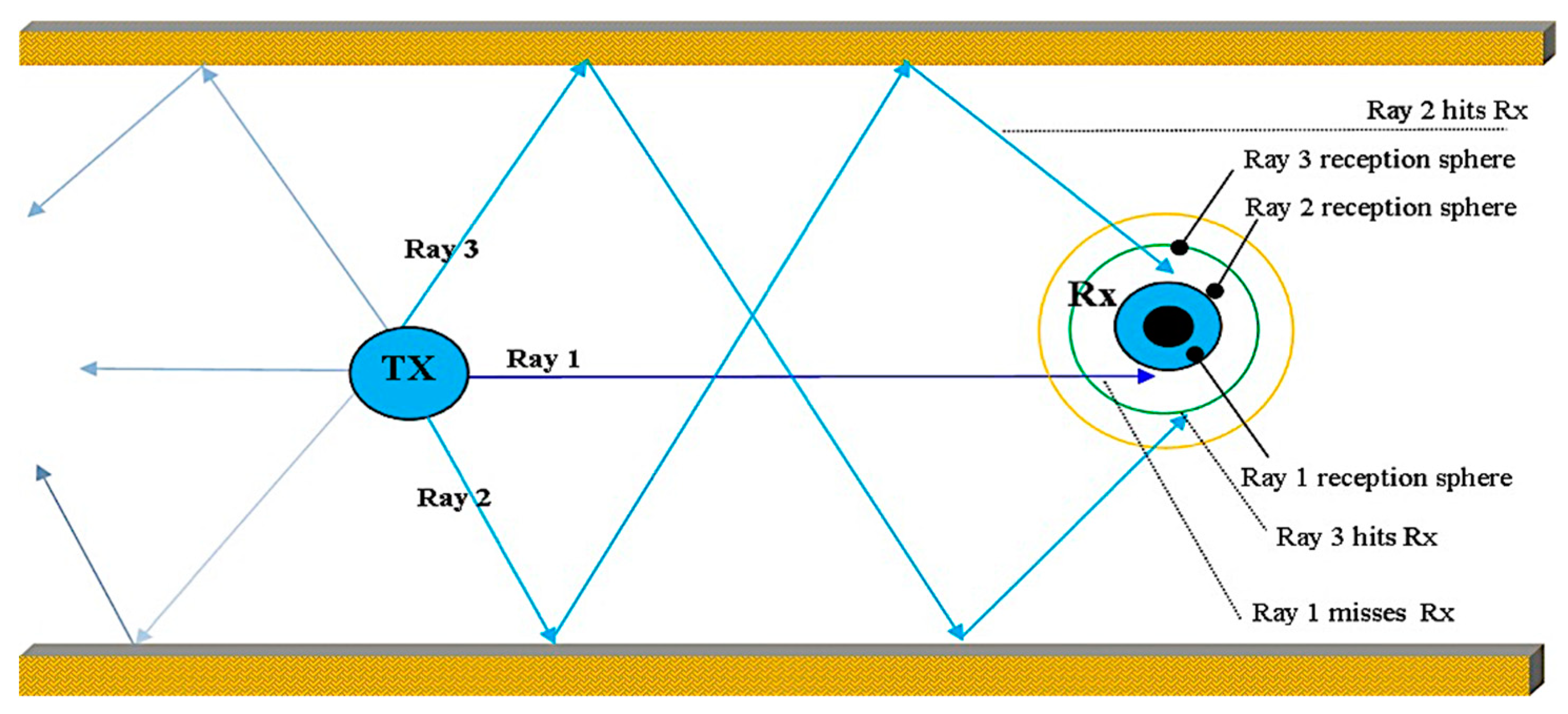
The SBRT technique is a high frequency asymptotic technique. It was developed by Ling et al. to compute the “radar cross section of cavities” [22], and the updated version is extended to detect the stature of targets [23]. Nowadays, SBRT is used for modeling radio wave with multiple reflection and scattering. In the SBRT method, rays or ray sets are emitted from the TX in all directions, and reflected from several objects before reaching the Rx. The targeted Rx is identified by a sphere with center point at Rx and whose spherical area is marked based on the path length of a specific ray and on the resolution angle between neighboring rays. The entire process is illustrated in Figure 2.

The complexity of the SBRT method mainly depends on the obstacles involved and the ray shooting angle resolution.

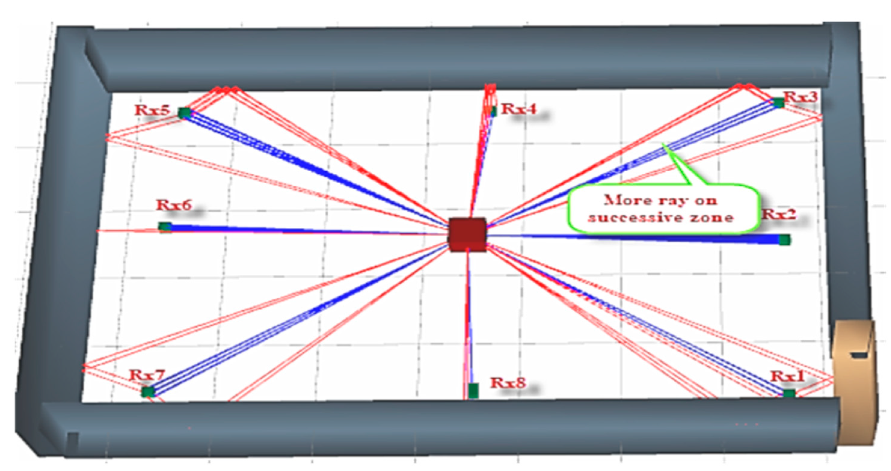
As shown in Figure 3, RT is performed using the SBRT method between one TX and eight Rx. For the conventional SBRT procedure, all the Rx received a few number of LOS and NLOS paths.

3.2. Conventional RT Method Limitations

In the conventional RT methods, rays are emitting in all directions. Every ray performs 3-D RT calculations. The calculations will show whether the traced ray could be intercepted by the receiver sphere, or not. Hence numerous launched rays are needed in order to obtain reasonable results. As a result, the methods usually require huge resources and high computational time.

3.3. Proposed Efficient Ray Tracing Method

The proposed efficient 3-D RT method has six phases. For the purpose of identifying the vector direction of a launching ray, the angle on the horizontal plane, measured from a reference direction, is called the horizontal angle. The azimuthal angle on a vertical plane, measured from a reference direction, is called the vertical angle. These two angles determine the vector direction of the ray.

In Phase 1, the appropriate graphical representation of the layout is determined, locating all obstacles, mobile stations, and base station, within the actual geometry of the environment. The closeness of the design to the measurement environment is important for accurate simulation results.

In Phase 2, ray launching is performed from the transmitter to the environment, including effects of reflection, refraction, and diffraction. In the simulation, the rays are launched at regular horizontal angle steps of (π/60) radian. For each of the horizontal angle, rays are also launched at regular vertical angle steps of (π/180) radian. Note that, in the conventional method, the horizontal angle steps are also (π/180) radian, which result in about three times more rays to be calculated, compared to our method.

In Phase 3, calculations are made to determine which of the rays in Phase 2 are successful in reaching a receiver. The horizontal and vertical angles for these successful rays are noted for processing in the next phase.

In Phase 4, for each of the successful rays, eight more new rays are generated at vertical angles which are 0.25, 0.50, 0.75, and 1.0 radians above and below the ray vector (at the same horizontal angle of the vector). These additional rays are more like to accepted by receivers and constitute the predefined rays in the next phase.

In Phase 5, all the successful rays in Phase 4, together with the additional eight new rays for each of them (four rays above and four rays below) are combined in the final ray launching. In case there are overlapping rays, only one distinct ray is considered.

In Phase 6, every launch ray from Phase 5 are traced, blue mark line for LOS, and red mark line for NLOS. Every ray outcome is stored for future analysis.

The two main advantages of our method are, firstly, the number of launched rays are drastically reduced, because the number of horizontal angle steps are much lower. The reduced steps have been found not to effect on the ray tracing results. Secondly, because we launch more rays in the proven favorable directions, we can expect more rays to be captured by the receivers.

Figure 4 shows that RT performed using the proposed method between one TX and eight Rx; however, for the proposed method, simulating all the Rx received a sufficient number of LOS and NLOS paths for good RSSI. It is clear from Figure 4 that successful angle steps launch more rays that contribute to the receivers.

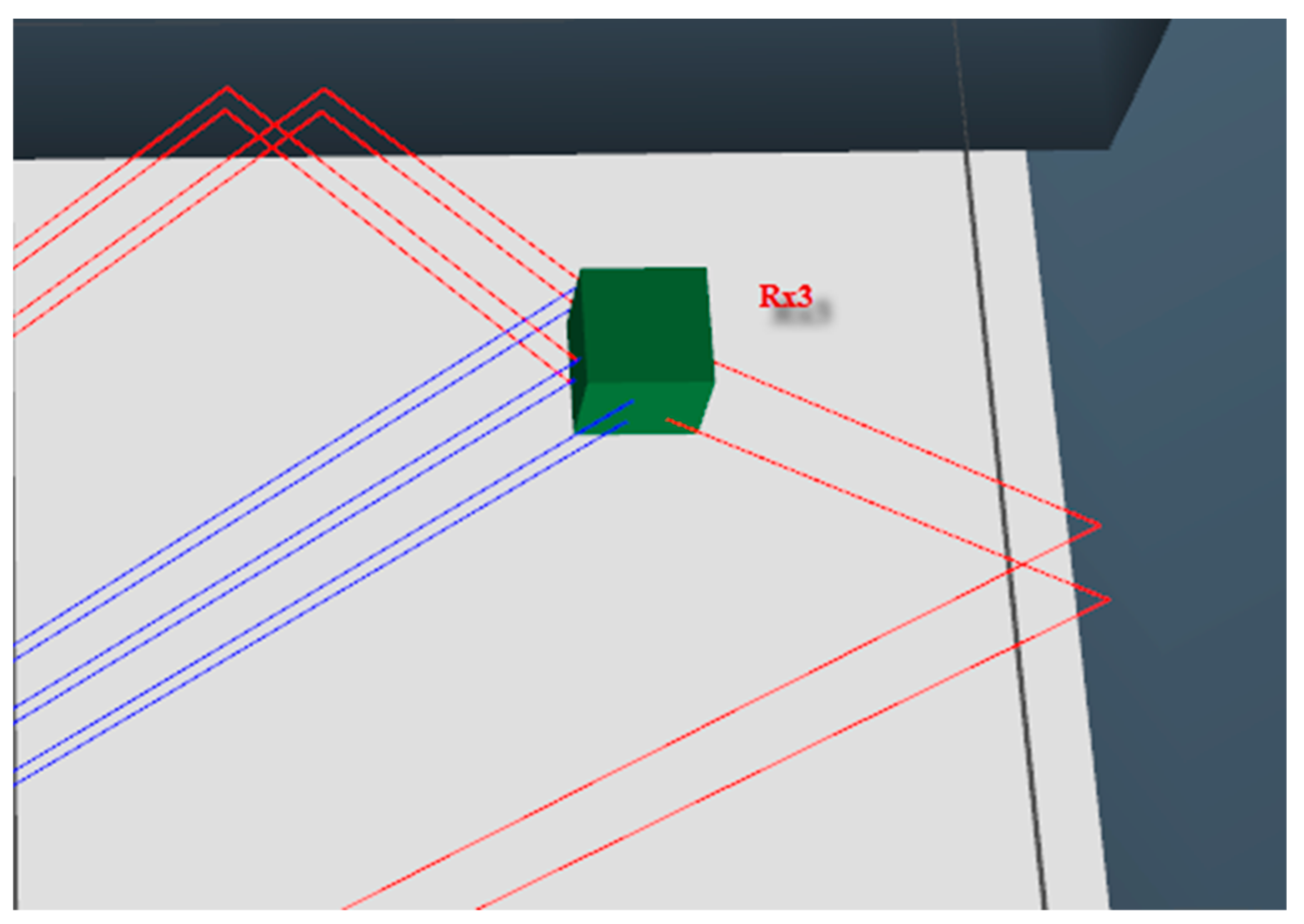
Figure 5 shows the zoom-in view of Rx3 receiver with multiple received rays. The receiver Rx3 receives six LOS and also six NLOS paths. All the ray paths received by Rx3 are actively contributing in calculations, so the RSSI will be more realistic. In summary, the proposed method provides good coverage to the mobile station, which is more essential for a higher frequency.

Proposed RT Method Complexity Analysis

The complexity of 3-D RT is low as only predefined rays are finally launched. The lower number of launching rays gives better accuracy even under a higher level of reflections. Moreover, less computational resources can easily handle this method. In the conventional method more rays shoot in all directions, so the complexity of calculations increases massively. Our method uses less time and therefore less computational complexity. The time is given by the following Equation (7).

$$\mathrm{Computational}\mathrm{time}=\left[\left\{\left(\frac{2\pi }{\Delta \varphi }\right)\times \left(\frac{\pi }{\Delta \theta }\right)\right\}+\left(n\times 4\right)\right]\times t$$

(7)

The symbols $\Delta \varphi$, $\Delta \theta$, $n$, and t mean: ray launching horizontal angle step, ray launching vertical angle step, number of successful directions in pre-calculation in Phase 3, and average simulation time (ns) for a ray, respectively. For Omni directional base station, 360-degree angles need to be divided by launching horizontal step size as it launches the rays in 360-degree angles, but for horn antenna it is controlled by the beamwidth. Here, that ray launching horizontal steps size ($\Delta \varphi =\frac{\pi }{60}$) which reduces the number of launching rays in Phase 3 drastically. In the conventional method, for $\Delta \varphi$ has several values, such as $\frac{\pi }{90}$, $\frac{\pi }{180}$, and $\frac{\pi }{360}$, and these increase the number of launching rays drastically.

3.4. Reflection

The dimensions of indoor walls are larger compared with the wavelength of mmWave. Moreover, in the same medium, the reflection coefficients constant is calculated by using the “Fresnel equation” [24]. Following the Fresnel standard mathematical model, reflection coefficients constant of perpendicular and parallel polarizations, ${\tau }_s$ and ${\tau }_p$ respectively can be calculated with Equations (8) and (9) using the wave impedance as presented below:

$${\mathsf{\Gamma }}_s=|\frac{Z_{2}cos{\theta }_i-Z_{1}cos{\theta }_t}{Z_{2}cos{\theta }_i+Z_{1}cos{\theta }_t}{|}^2$$

(8)

$${\mathsf{\Gamma }}_p=|\frac{Z_{2}cos{\theta }_t-Z_{1}cos{\theta }_i}{Z_{2}cos{\theta }_t+Z_{1}cos{\theta }_i}{|}^2$$

(9)

The angles ${\theta }_i$ and ${\theta }_t$ are used to express the incident and refracted angles, and $Z_1$ and $Z_2$ are the impedances of first and second media, respectively. The impedance value depends on relative permittivity ${\epsilon }_r$ of the obstacle and the permeability ${\mu }_0$ for blank and non-magnetic media of the building material. The conductivity σ is presumed to be very low for non-conducting building materials, such as concrete, brick, and glass. Figure 6 shows the graphical presentation of reflection.

Furthermore, by using Snell’s law the refraction coefficients are given by Equations (10) and (11).

$${\mathsf{\Gamma }}_s=|\frac{cos{\theta }_i-\sqrt{{\epsilon }_r-si{n}^2{\theta }_i}}{cos{\theta }_i+\sqrt{{\epsilon }_r-si{n}^2{\theta }_i}}{|}^2$$

(10)

$${\mathsf{\Gamma }}_p=|\frac{{\epsilon }_{r}cos{\theta }_i-\sqrt{{\epsilon }_r-si{n}^2{\theta }_i}}{{\epsilon }_{r}cos{\theta }_i+\sqrt{{\epsilon }_r-si{n}^2{\theta }_i}}{|}^2$$

(11)

The parameters ${\theta }_i$ and ${\epsilon }_r$ mainly determined the reflection coefficient. The value of ${\epsilon }_r$ relies on the frequency spectrum of electromagnetic signal and the indoor medium properties. Nevertheless, for the higher frequency 28 GHz band, it is hard to get the standard nominal value of permittivity of indoor environment for the RT method. The permittivity value is set to six for frequencies of 900 to 1900 MHz range in Reference [25] and the permittivity values for several indoor materials presented in Reference [26]; although the frequency band 28 GHz is not included. The building materials and carrier frequency play vital roles for ${\epsilon }_r$: The value of ${\epsilon }_r$ changes significantly depending on the building properties. Moreover, some glasses have ${\epsilon }_r$ values of 6.08 and 8.9 at 5 GHz, and 62.4 GHz frequency, respectively. Similarly, some brick has ${\epsilon }_r$ values of 4.5 and at 2 GHz, but 3.95 at 60 GHz frequency band, respectively. Recently, Samsung Electronics estimated values of ${\epsilon }_r$ and $\sigma$ for the RT simulation at 28 GHz band. Estimations for building concrete are ${\epsilon }_r$ = 6.5 and $\sigma$ = 0.668 [27]. In the simulation for both SBRT and the proposed method, ${\epsilon }_r$ values are considered limited from 6 to 8 with respect to building material properties [27,28,29].

3.5. Diffraction

The diffraction coefficient values including vertical and horizontal angles are calculated by using the wedge model [30]. Even though the RSSI of the diffracted signal is much lower than the main incident ray, diffraction is a very significant factor for WCS as it assists rays to reach the shadowed zone. In addition, it is complicated to simplify diffraction in the RT method, as all the primary ray objects become subordinate source points that produce several diffracted rays and raise the computational complexity. To control this issue, an updated Luebber model has been used to estimate the diffraction coefficient [30,31]. Based on the UTD, the field $E_{GTD}$ at specific point is expressed in Equation (12) [32].

$$E_{GTD}=E_0\frac{e^{-jk{p}^{\prime }}}{p^{\prime }}D\begin{array}{c}\perp \\ \parallel \end{array}\sqrt{\frac{p^{\prime }}{p\left(p^{\prime }+p\right)}}{e}^{-jkp}$$

(12)

The $E_0$ is the origin amplitude, k is the wave number expressed, $p$ is the calculated distance among the Tx and diffraction point, $p^{\prime }$ is the distance between the diffraction edge and Rx, and $D\begin{array}{c}\perp \\ \parallel \end{array}$ is the diffraction. For non-conducting obstacles, coefficients for every polarization are calculated using Equation (13).

$$\begin{array}{c}D\begin{array}{c}\perp \\ \parallel \end{array}=\frac{-e^{(-j(}k(p+p{}^{\prime })+\pi /4))}{2n\sqrt{2\pi k}\mathit{sin}\beta }X\{\frac{F(kL{a}^{+}(\varphi -\varphi {}^{\prime }))}{\mathit{t}\mathit{a}\mathit{n}[(\pi +\varphi -\varphi {}^{\prime })/2n]}+\frac{F(kL{a}^{-}(\varphi -\varphi {}^{\prime }))}{\mathit{t}\mathit{a}\mathit{n}[(\pi +\varphi -\varphi {}^{\prime })/2n]}\\ +\mathsf{\Gamma }\begin{array}{c}\perp \\ 0 \parallel \end{array}\frac{F(kL{a}^{-}(\varphi +\varphi {}^{\prime }))}{\mathit{t}\mathit{a}\mathit{n}[(\pi +\varphi -\varphi {}^{\prime })/2n]}+\mathsf{\Gamma }\begin{array}{c}\perp \\ n \parallel \end{array}\frac{F(kL{a}^{+}(\varphi +\varphi {}^{\prime }))}{\mathit{t}\mathit{a}\mathit{n}[(\pi +\varphi +\varphi {}^{\prime })/2n]}\}\end{array}$$

(13)

The reflection coefficients $\mathsf{\Gamma }\begin{array}{c}\perp \\ 0 \parallel \end{array}$ and $\mathsf{\Gamma }\begin{array}{c}\perp \\ n \parallel \end{array}$ are used for both types of polarization. The forward and backward incident angles expressed by $\varphi$ and $(n\pi -\varphi$), respectively; $L=\left(p{p}^{\prime }\left(p+p^{\prime }\right)\right);$ $a\pm \left(\beta \right)=2cos2\left[\left(2n\pi N\pm -\beta \right)\right]/2]; \beta =\varphi \pm {\varphi }^{\prime };$ and $N\pm$ are the integers to satisfy Equation (12).

Figure 7 expresses the schematic of diffraction with notations. The simulation tool has been developed for both horizontal and vertical diffractions at every ray direction. This drawback of diffraction is presented in Reference [33] for the 28 GHz frequency band.

3.6. Ray Tracing Formula

In indoor radio wave propagation, the rays experience several reflections and diffractions before reaching the receiver. Here the electric field intensity ${\mathrm{E}}_n$ is calculated using Equation (14) [31].

$${\mathrm{E}}_n={\mathrm{E}}_{\mathrm{in}}\left(Q_n\right)\left({\displaystyle \prod }_{i=0}^{a_n}{R}_{in}{A}_{rin}\right)\left({\displaystyle \prod }_{j=0}^{b_n}{T}_{jn}{A}_{tjn}\right) \left({\displaystyle \prod }_{m=0}^{c_n}{D}_{mn}{A}_{dmn}\right)e^{-jk{s}_n}$$

(14)

The term ${\mathrm{E}}_{\mathrm{in}}\left(Q_n\right)$ is used to express the incidence of electric field for the first scattering point. The terms $a_n, b_n, and c_n$ are the number of reflections, transmissions, and diffractions which take place one after another. The terms $R_{in}, T_{jn}, and D_{mn}$ express associated dyadic reflection, the transmission, and diffraction coefficient, respectively. The terms $A_{rin}, A_{tjn}, and A_{dmnn}$ express related spreading factors. S_n is the cumulative distance crossed by a ray. Moreover, for multichannel propagation, Rx receives multiple rays. For this environment, cumulative electric field intensity E_total is the accumulation of all rays, as calculated using Equation (15).

$${\mathrm{E}}_{total}={\displaystyle \sum }_{n=0}^M {\mathrm{E}}_{\mathrm{in}}\left(Q_n\right)\left({\displaystyle \prod }_{i=0}^{a_n}{R}_{in}{A}_{rin}\right)\left({\displaystyle \prod }_{j=0}^{b_n}{T}_{jn}{A}_{tjn}\right) \left({\displaystyle \prod }_{m=0}^{c_n}{D}_{mn}{A}_{dmn}\right)e^{-jk{s}_n}$$

(15)

The total number of rays reaching a Rx is expressed by the symbol M.

To get the transmitted power $P_t$ from the TX, antenna pattern, and $Q_n$ from RT, ${\mathrm{E}}_{\mathrm{in}}\left(Q_n\right)$ can be estimated by the Equation (16) [34].

$${\mathrm{E}}_{\mathrm{in}}\left(Q_n\right)=\frac{E_0\sqrt{G_m^{\prime }}}{p_n} \tilde{a}{}_m$$

(16)

The $E_0=\sqrt{\frac{n_0}{4\pi }}{P}_t{G}_t$ symbolizes the electric field intensity 1 meter from the base station in the direction of highest antenna gain [35]. The $n_0$ expresses intrinsic impedance, $G_t$ symbolizes antenna directivity, $G_m^{\prime }$ means normalized antenna gain in the direction of $Q_n$. The $\tilde{a}{ }_m$ express antenna polarization in the direction of $Q_n$. The $p_n$ also express the length of $Q_n$ from the base station. The term ${\mathrm{E}}_n$ symbolizes the ray field strength of the mobile station. The accurate estimate voltage (Vrn) is dependent on the antenna type and polarization of the mobile station. Considering the model of linear antenna, the term V_rn is expressed in Equation (17).

$$V_{rn}=\sqrt{\frac{{\lambda }^2{G}_{rn}{R}_0}{4\pi }}\left({\mathrm{E}}_n.\tilde{a}{}_{rm}\right)e^{j\varphi }$$

(17)

The term $\lambda$ means the wavelength, $G_{rn}$ is mobile station antenna gain in the ray receiving angle, $R_0$ is mobile station characteristic impedance, the $\tilde{a}{ }_{rm}$ is Rx antenna polarization in the ray receiving angle, and $e^{j\varphi }$ is static-phase shift presented by Rx antenna. Finally, the entire received power RSSI is given by Equation (18) [36].

$$\begin{array}{l}{P}_r=\frac{\left|{{\displaystyle \sum }}_{n=0}^M{V}_m\right|{}^2}{R_0}=\frac{{\lambda }^2}{4\pi n_0}|{\displaystyle {\displaystyle \sum }_{n=0}^M}\left(E_n.{\tilde{a}}_{rn}\right)\sqrt{G_{rn}}{|}^2\\ =\frac{{\lambda }^2}{4\pi n_0}|{\displaystyle {\displaystyle \sum }_{n=0}^M}\frac{E_0{e}^{-jk{s}_n}\sqrt{G_{rn}{G}_{tn}^{\prime }}}{P_n}{\tilde{a}}_{tn}\left({\displaystyle {\displaystyle \prod }_{i=0}^{a_n}}{R}_{in}{A}_{rin}\right)\left({\displaystyle {\displaystyle \prod }_{j=0}^{b_n}}{T}_{jn}{A}_{tjn}\right)\left({\displaystyle {\displaystyle \prod }_{m=0}^{c_n}}{D}_{mn}{A}_{dmn}\right){\tilde{a}}_{rn}{|}^2\end{array}$$

(18)

here the total length of the valid path is mentioned by M.

3.7. Server Specifications and Simulation Parameter Configuration

The relevant parameters were configured in the simulation as measurements to compare the output with measurement data. To match the base station and mobile station setup with measurement, a horn antenna was used as TX, and an omnidirectional antenna as Rx. The simulation server had a Y0M88AA#UUF configuration: The operating system is MS-windows 2016 server version, 64-bit, and version no. 10.0*; processor is Core i7, Eight-Core CPU, and 16 Logical CPU(s); RAM is 16 GB; and the internal graphics card is 4 GB GDDR5. The latest technologies were used for simulator development: IDE Visual Studio 2017; framework WPF; programing language visual C#; and the database MS-SQL server 2017 standard edition. In this research, the conventional SBRT and the proposed methods implementation were done in the in-house developed simulator one by one. This tool executed RT dynamically using configurable parameters. Mainly, RT simulation depends completely on the configuration parameters [37,38]. The same values of parameters for SBRT and proposed algorithms were used. For this simulation to generate signal, a horn antenna TX was used, with an operating frequency of 28 GHz. Higher operational frequencies can provide high RSSI but cannot cover a large area because of the high PL. Normally, the PL increases because of larger distance, frequency, reflections, etc. Thus to cover large indoor areas such as an indoor stadium, lower frequency or multiple antenna in higher frequency are used. The TX was placed in Room 1 as per layout point of the measurement scenario. The horn TX was placed in the center to cover the whole area at signal base station. However, the horn antenna can be placed anywhere with respect to the beamwidth to cover the dense mobile station area properly. The TX height is a very important factor in simulation: Reflection mainly depends on TX height; a higher base station bears fewer numbers of reflections. The base station height should be below ceiling height. For the calculation, 80 pixels was counted as a meter. By using meter for pixels, it is easy to control the layout area in simulation especially in zooming. To cover a larger area in simulation, a lower number of pixels can be considered as a meter. In this RT simulation, the base station height was 1.5 meters and 25 dBm powers were transmitted from it. Here, the reflections were controlled by its limit value; for this scenario, a maximum of 25 numbers of reflections are counted for every single ray. By increasing the reflection number in simulation, it is possible to cover more Rx, but it increases the computational time; although, a higher frequency does not support a higher number of reflections because it increases the PL. If the PL is so high, then the path is conditionally ignored in simulation because of the Rx sensitivity limit. One-pixel ray thickness is considered in signal visualization. For small indoor areas one-pixel is good enough to express the LoS and NLoS paths.

The details specification of the WCC P15a environment materials corresponding to Figure 1 is shown in

Table 3. Specifications of the experimental environment [39].

Obstacle	Material	Height (m)	Relative Permittivity	Refractive Index
Wall	Brick	2–4.5	5.2	1.7–2.2
Window	Glass	1–1.5	3.7	1.50–1.92
Door	Wood	1.75–2.75	3	2.2
Table	Wood	1.1	3	2.2
Partition	Plastic board	1.83	2.8	1.46–1.55

.

4. Validation of Ray Tracing Results

The RT simulation and its validation with respect to measurement is described in this section. The objective of this research was to validate the simulated Rx point with the measurement from a similar distance of TX location by appropriate comparison of both results. The simulation 3-D layout design included the building architecture and features in the simulator. The simulation was performed by the in-house simulator software using the SBRT and proposed methods. As per RT features, the maximum number of the rays hit upon the indoor objects and walls. After a hit, it was reflected, and the reflecting and tracing continued until the maximum number of reflections allowed was reached. For each multi-channel ray, the RT considered reflections and penetrations effects depending on the GO and UTD. The simulation calculated the mmWave RSSI and PL, considering the contributed rays received at mobile station points [40]. At 28 GHz frequency mmWave propagation feature to trace paths up to the higher PL, −150 dB parameterized as lower receiver sensitivity for RT simulation. The ray path was ignored if ray reflections reached the limit or RSSI dropped below the lower receiver sensitivity of −150 dB.

In this study, actual measurement was conducted at WCC P15a and simulation was done on its layout using both SBRT and proposed RT methods for indoor radio propagation. Generally, normal windows and doors, transparent windows and doors, and walls were included in the simulation scenario. Small obstacles were ignored to simplify the scenario. Some practical issues are raised to estimate the permittivity of obstacles because of different types of wooden wall, the different compositional concrete obstacles, and different types of ceiling. Therefore, in these circumstances, standard values of an environmental object given in Reference [41] were incorporated in the simulation. The simulation layout was designed as similar, considering several big rooms as measurement layout. The TX was placed inside Room 1 and multiple mobile stations positioned in as per measurement layout.

The frequency spectrum had a direct propagation effect depending on the indoor environment obstacle materials. The permittivity and conductivity values of obstacle materials were changed with frequency bands [42,43,44], but these standard values of parameters are for 28 GHz.

The graphical simulation output of the WCC P15a layout using SBRT is showed in Figure 8, which shows that it has more reflections; hence, PL, propagation times will be higher and RSSI will be lower. It is also noticeable that the coverage is not good because a few rays contributed to the Rx, mostly those bearing higher reflections. If few number of rays contribute to Rx, then RSSI will be lower. Moreover, some Rx receive multiple rays but most of them are due to multiple reflections, which contain higher PL that directly effect on RSSI.

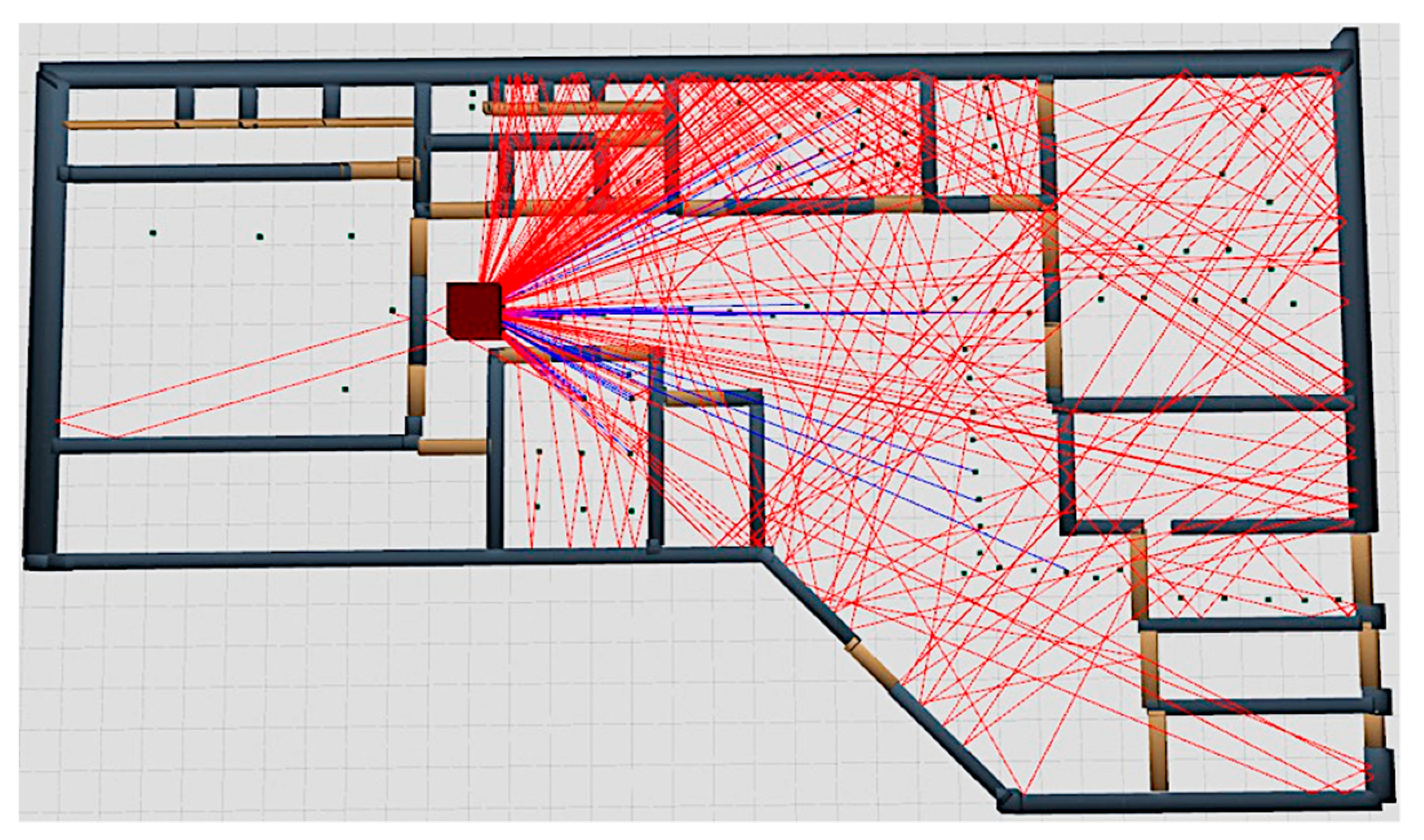
The graphical simulation output of the WCC P15a layout using the proposed method is showed in Figure 9. It has a lower number of reflections, therefore, PL propagation times will be lower and RSSI will be higher. It is also noticeable that the coverage is good because more rays contributed to the Rx, mainly those from a lower number of reflections. If a higher number of rays contribute to Rx, then RSSI will be high. However, some Rx receive multiple rays mostly from lower reflections, which contain lower PL that count as a positive factor to RSSI. By comparing output data of the proposed method and measurement with respect to RSSI and PL, there is good agreement.

The average RSSI difference between measurement and the simulation data using the SBRT method is 5.65 dBm for the WCC P15a scenario. The minimum and maximum difference of RSSI between measurements and the RT simulation using the SBRT method are 1.05 and 11.10 dBm, respectively. The maximum RSSI difference takes place for large obstacle or the contributed rays contain the higher number of reflected rays. The association of the RSSI of measurement and the SBRT method with respect to several Rx from multiple locations is illustrated in

Table 4. Comparison of received signal strength indication (RSSI) data among measurement, SBRT method, and proposed method.

Mobile Station	Measurement RSSI (dBm)	SBRT Method RSSI (dBm)	Proposed Method RSSI (dBm)
Rx33	−67.3	−69.63	−65.97
Rx34	−67.7	−65.96	−66.72
Rx35	−67.8	−57.67	−62.85
Rx38	−68.1	−72.71	−68.99
Rx39	−67.6	−74.47	−69.47
Rx41	−68.1	−70.07	−70.05
Rx42	−72.6	−74.20	−74.20
Rx44	−71.8	−74.46	−74.45
Rx45	−71.5	−75.30	−75.69
Rx48	−70.4	−69.35	−69.21
Rx49	−70.7	−80.34	−73.44
Rx50	−71.1	−75.56	−72.31
Rx51	−70.7	−78.08	−75.53
Rx72	−66.5	−72.40	−70.18
Rx74	−65.5	−79.84	−69.84
Rx77	−66.8	−77.90	−68.41
Rx83	−61.6	−68.07	−55.55

.

Correspondingly, the average RSSI difference between measurement and the simulation using the proposed method at the same scenario in the same frequency is 2.7 dBm. The below three dBm average difference within measurement and simulation is indicative of the acceptable RT modeling. The minimum and maximum RSSI difference between measurement and simulation using the proposed method are 0.89 and 6.05 dBm, respectively. Moreover, the higher RSSI difference is found in some points because of sudden obstacles. However, for the proposed method, even in an obstructed worst-case scenario, the RSSI difference is considerable between measurement and the proposed method. The association of the RSSI within measurement and proposed method, with respect to several Rx from multiple locations is shown in Table 4.

The line graph in Figure 10 represents the line view of RSSI within the three sets of output. The measurement RSSI data is taken as the standard data. In the RSSI similarity of SBRT method with standard data, mobile stations Rx48, Rx42, Rx34, Rx41, Rx33, Rx44, Rx45, Rx50, and Rx38 illustrates the moderate relationship, respectively. The average difference of SBRT method RSSI with the standard is 2.69 dBm for those data. Inversely, in the SBRT mobile stations Rx72, Rx83, Rx39, Rx51, Rx49, Rx35, Rx77, and Rx74 demonstrate a distance relationship. The average dissimilation of SBRT method RSSI with the standard is 8.97 dBm for those data. On the other hand, to the higher RSSI matching trend of proposed method, mobile stations Rx38, Rx34, Rx48, Rx50, Rx33, Rx42, Rx77, Rx39, Rx41, Rx44, Rx49, Rx72, Rx45, Rx74, Rx51, and Rx35 illustrate a very good agreement with the respective standard data. The average difference of proposed method with the standard is 2.5 dBm for those data. Moreover, all the mobile stations except Rx83 express the outstanding agreement with the standard data. The mobile station Rx83 demonstrates a distance relationship from the standard data because of the sudden appearance of obstacles and reflections.

According to the higher similarity of simulation considering the average RSSI difference with measurement less than 5 dBm, 9 numbers of Rx are in SBRT; and 16 numbers of Rx are found in the proposed method. There is a lower similarity of simulation considering the average RSSI difference with measurement is greater than 5 dBm: Eight numbers of Rx are found in SBRT; and only one Rx is found in the proposed method. With the analysis from Table 3 and Figure 3, Figure 4, and Figure 10 for RSSI comparison, it is seen that the proposed method output illustrates a higher agreement with measurement data than the SBRT output data.

The average difference of PL with the measurement and SBRT simulation is 8.83 dB. The minimum and maximum difference of PL within the measurement and SBRT simulation are 0.96 and 19.16 dB, respectively. The comparison of measurement and SBRT simulation for several Rx from different points are expressed in Table 4. The average difference between the measurement and proposed method simulation is 3.83 dB for this layout. The minimum and maximum difference of PL within the measurement and proposed method are 0.30 and 9.71 dB, respectively. However, the higher PL difference is found in some Rx because of the sudden appearance of objects which give rise to higher reflected rays. Moreover, even in worst-case scenarios, the difference in PL between the measurement and proposed method is considerable. The association of the PL within the measurement and proposed method, with respect to several Rx from multiple locations are illustrated in

Table 5. The comparison of PL data using measurement, SBRT method, and proposed method.

Mobile Station ID	Measurement PL (dB)	SBRT Method PL (dB)	Proposed Method PL (dB)
Rx33	86.68	69.96	76.97
Rx34	87.08	67.92	84.72
Rx35	87.18	81.91	85.28
Rx38	87.48	78.47	82.28
Rx39	86.98	80.07	82.47
Rx41	87.48	78.20	80.05
Rx42	91.98	81.96	88.20
Rx44	91.18	83.96	88.95
Rx45	90.88	73.35	88.24
Rx48	89.78	88.34	86.21
Rx49	90.08	80.56	84.94
Rx50	90.48	84.74	84.81
Rx51	90.08	86.40	86.53
Rx72	85.88	76.40	86.18
Rx74	84.88	85.84	85.84
Rx77	86.18	75.90	82.41
Rx83	80.98	73.07	78.55

.

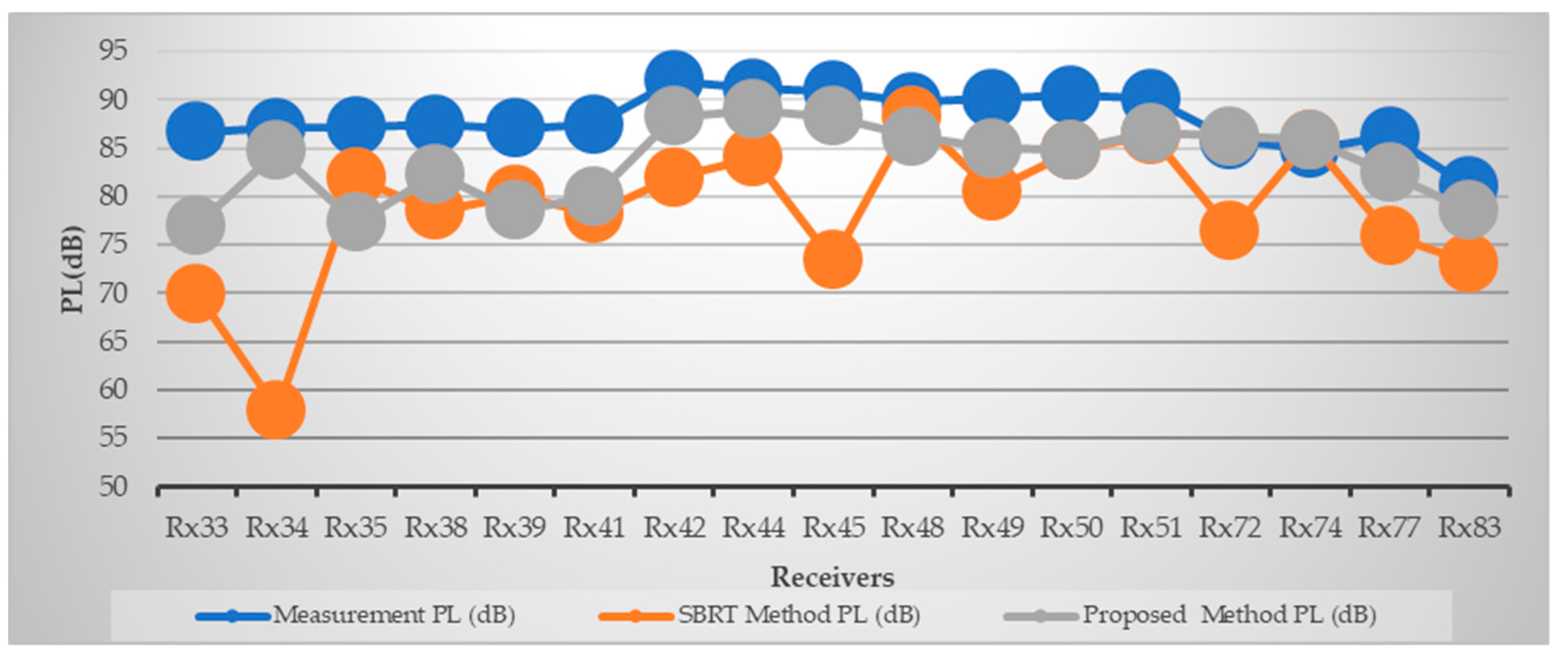
Figure 11 illustrates the line graph of PL comparison among the three sets of output data, with the measurement data as the standard data. The PL similarity of SBRT method with standard data for mobile stations Rx74, Rx48, Rx51, Rx35, Rx50, and Rx39 which illustrates the moderate relationship, respectively. The average difference of RSSI between SBRT method and standard data is 4.0 dB. In the SBRT mobile stations Rx44, Rx83, Rx38, Rx41, Rx72, Rx49, Rx42, Rx77, Rx33, Rx45, and Rx34, the distance relationship can be seen. The average difference between the SBRT method RSSI with the standard is 11.47 dB for those data. On the other hand, to the higher PL matching trend of the proposed method, mobile stations Rx72, Rx74, Rx35, Rx44, Rx34, Rx83, Rx45, Rx51, Rx48, Rx77, Rx42, Rx39, Rx49, Rx38, and Rx50 illustrate the good agreement with the standard data. The average difference for PL between the proposed method and the standard is 3.20 dB. In the proposed method, mobile stations Rx41 and Rx33 illustrate the distance relationship respectively with PL from the standard. Here, the average PL difference is 7.48 dB for those mobile stations. According to the higher similarity of simulation, considering the average PL difference with measurement is less than 7 dB, 6 receivers are in SBRT; and 15 receivers are found in the proposed method. There is a lower similarity of considering the average PL difference with measurements greater than 7 dB: 11 receivers are found in SBRT; and 2 receivers are found in the proposed method. With the analysis Table 5 and Figure 3, Figure 4 and Figure 11 for PL comparison, it is clear that the proposed method shows a higher agreement with measurement data.

Figure 12 represents the ray propagation time comparison between the SBRT method and proposed method. Our proposed method propagation time is less than those on SBRT method. Hence overall, the proposed method took much less time than the conventional method.

The proposed method is capable of generating a power delay profile for every mobile station. For example, some mobile station power delay profiles are presented in

Table 6. Power delay profile for Rx41, Rx48, and Rx72 based on proposed method.

Mobile Station.	Path SL.	Proposed Method RSSI (dBm)	Proposed Method Propagation Time (ns)
Rx41	1	−64.87	1.52
	2	−65.72	1.79
	3	−65.89	2.12
	4	−68.11	3.52
	5	−70.02	3.91
	6	−76.57	7.18
	7	−78.29	8.25
Rx48	1	−69.71	3.69
	2	−70.13	4.25
	3	−73.54	6.26
	4	−78.63	8.89
	5	−79.21	10.83
Rx72	1	−75.45	5.38
	2	−85.98	54.48

. In calculation, we combine the mobile station received paths (LOS, NLOS), considering phase using vector sum to get specific mobile stations RSSI. We compared this RSSI with the measurement data and they agree. However, this detail simulation data shows that our method is also appropriate to verify advance measurement data. The measurement campaign, where multi-array antenna is used, can produce path detail at the mobile station, which can be used to validate power delay profile data.

Our proposed RT method can provide more accurate site specific results compared to the empirical statistical method. The main disadvantage of the empirical statistical method is lower accuracy as it does not consider the scenario-based propagation prediction. Our method belongs to site specific models, so it overcomes the limitations of statistical models. Our method is faster, as our calculation phase helps to overcome the computational limitation of the site specific methods. The RL phase optimization is a good contribution in proposed RT [45,46,47,48]. The appropriate use of RL phase in the proposed method makes it more efficient. The number of rays launching for the proposed method are much less than the SBRT method. Therefore, to get good coverage by using RL pre-defined region is the main contribution of our method.

5. Conclusions

This paper presents the 3-D RT simulation results for radio propagation prediction under an indoor environment. Although practical measurement provides accurate judgment of performance, a huge amount of resource are needed. Hence, computerized simulations tools are helpful. The conventional RT simulation takes higher computational time to cover whole azimuth and elevation resolution of indoor scenario. Using the proposed new model, more rays are allowed in some potential zones and not in all directions, which reduces the computational complexity without reducing valid paths between TX and Rx. For the validation of the proposed method, the simulation result in WCC P15a was compared with the measurement RSSI, PL data from real site. Additionally, for novelty, the proposed efficient method, the conventional SBRT method simulation results have been also compared with the same measurement data. Based on the comprehensive comparison, acceptable agreement is found for the proposed method. The results of this research are expected to guide further research into 28 GHz mmWave indoor mobile networks systems.