An Efficient Streaming Accelerator for Low Bit-Width Convolutional Neural Networks
by
Qinyu Chen
1, 
Yuxiang Fu
1,*,
Wenqing Song
1,
Kaifeng Cheng
1,
Zhonghai Lu
2, 
Chuan Zhang
3 and
Li Li
1,* 1
School of Electronic Science and Engineering, Nanjing University, Nanjing 210093, China
2
KTH-Royal Institute of Technology, 10044 Stockholm, Sweden
3
National Mobile Communications Research Laboratory, Southeast University, Nanjing 210096, China
*
Authors to whom correspondence should be addressed.
Electronics 2019, 8(4), 371; https://0-doi-org.brum.beds.ac.uk/10.3390/electronics8040371
Submission received: 25 February 2019
/
Revised: 15 March 2019
/
Accepted: 22 March 2019
/
Published: 27 March 2019
(This article belongs to the Special Issue Convolutional Neural Network Design and Hardware Implementation for Real-Time Vision Applications)
Abstract
:Convolutional Neural Networks (CNNs) have been widely applied in various fields, such as image recognition, speech processing, as well as in many big-data analysis tasks. However, their large size and intensive computation hinder their deployment in hardware, especially on the embedded systems with stringent latency, power, and area requirements. To address this issue, low bit-width CNNs are proposed as a highly competitive candidate. In this paper, we propose an efficient, scalable accelerator for low bit-width CNNs based on a parallel streaming architecture. With a novel coarse grain task partitioning (CGTP) strategy, the proposed accelerator with heterogeneous computing units, supporting multi-pattern dataflows, can nearly double the throughput for various CNN models on average. Besides, a hardware-friendly algorithm is proposed to simplify the activation and quantification process, which can reduce the power dissipation and area overhead. Based on the optimized algorithm, an efficient reconfigurable three-stage activation-quantification-pooling (AQP) unit with the low power staged blocking strategy is developed, which can process activation, quantification, and max-pooling operations simultaneously. Moreover, an interleaving memory scheduling scheme is proposed to well support the streaming architecture. The accelerator is implemented with TSMC 40 nm technology with a core size of mm. It can achieve TOPS/W energy efficiency and TOPS/mm area efficiency at mW, which makes it a promising design for the embedded devices.
1. Introduction
Convolutional neural networks (CNNs) have been widely applied in a variety of domains [1,2,3], and achieve great performance in many tasks including image recognition [4], speech processing [5] and natural language processing [6]. With the renewal of the CNN models, larger and deeper structures promise the improving predicting accuracy [7]. However, the number of parameters also increases dramatically, resulting in unacceptable power dissipation and latency, which hinders the implementation of the Internet-of-Thing (IoT) applications like intelligent security systems.
The problems stimulate the research of both algorithms and hardware designs to pursue low power and high throughput. In terms of the former, one approach is to compress the model by pruning the redundant connections, resulting in sparse neural network [8]. Nevertheless, it also bears supplementary loads including the pruning, Huffman coding, and decoding. Another easier way is to simply train low bit-width CNN models, which each weight and activation can be represented with a few bits. For example, due to binarized weights and activations, Binarized Neural Networks (BNNs) [9] and XNOR-Net [10] use the bitwise operations instead of most of the complicated arithmetic operations, which could also achieve rather competitive performance. In addition, most of the parameters and data can be kept in on-chip memory, enabling greater performance and reducing external memory accesses. Nevertheless, such an aggressive strategy cannot guarantee accuracy. To compensate for this, the DoReFa-Net [11] adopts low bit-width activations and weights to achieve higher recognition accuracy. These delicate models are more suitable for mobile and embedded systems. Moreover, the hardware design of CNNs has also drawn much attention in recent years. Currently, Graphics Processing Units (GPUs) and TPU [12] have been the mainstay for DNN processing. However, the power consumption of GPUs, which are general-purpose compute engines, is relatively high for the embedded systems. The power consumption of another popular platform TPU is low, but the resource use is not satisfactory when processing most of the benchmarks.
Generally, there are three kinds of mapping methods from the layer computation to the computing units in hardware. First, previous research [13,14,15,16,17,18] maps CNN models onto an accelerator with only one computing unit, which will process the layers iteratively. This approach is called “one size fits all”. However, the fixed dimensions of one computing unit could not be compatible with all the layers with different dimensions, which leads to the resource inefficiency, especially in Fully Connected (FCN) layers [19]. Some recent works [20,21,22,23,24] focus on a parallel streaming architecture, which partitions a system into several independent tasks and runs them in parallel hardware [25]. In general, the partitioning includes task level and data level. Tasks are separated into sequential and parallel modules. Sequential modules are used to process different tasks, and parallel modules execute the same task based on different data. Based on this architecture, many accelerators are proposed. Yang et al. [20] adopt another mapping approach called “one to one”, which means that each layer is processed by an individual optimized computing unit. Thus it can achieve high resource use. Nevertheless, this approach requires more on-chip memory resources and control logic resources (i.e., configuration and communication logics). This is the second mapping way. Shen et al. [22] and Venieris et al. [23] both present a resource partitioning methodology for mapping CNNs on FPGAs. It can be regarded as a trade-off approach between “one size fits all” and “one to one”. These works can only construct an optimized framework for a specific CNN model at a time, but the framework cannot well apply to other models flexibly. In these works, a layer is the smallest unit of granularity during the partitioning. The computational workload balance is usually the primary concern, and the processing order may not according to the layer sequence of a CNN model, which probably causes too many data accesses to the external memory.
Recently, there is an increasing amount of research [17,18,21,26,27] focusing on the accelerators targeting on low bit-width CNNs. Wang et al. [17], Venkatesh et al. [26] and Andri et al. [18] all propose their own architecture for deep Binarized CNNs, working by “one size fits all” approach. In these works, the energy efficiency is better than that of conventional CNNs, since the complicated multiplications and additions are replaced by some simple operations. However, these three works do not take all kinds of layers acceleration into account. Umuroglu et al. build FINN [27] framework and its second generation FINN-R [28] framework for fast and flexible FPGA accelerators using a flexible heterogeneous streaming architecture, which works by the approach of “one to one”. Li et al. [21] design an FPGA accelerator which specifically targets at the same kind of low bit-width CNNs as ours. This accelerator consists of several computing units, each unit processes a group of layers, which is a trade-off approach. However, the processing time of each unit is not well balanced, which will reduce the throughput due to the large pipeline stalls. However, these designs usually ignore the design of layers except Convolutional (CONV) layers and FCN layers, and need extra hardware to support those layers like batch-normalization, activation, quantification, and pooling operation, which brings extra overheads.
To overcome these problems, we propose an efficient, scalable accelerator for low bit-width CNNs based on a parallel streaming architecture, accompanied by different optimization strategies, aiming at reducing the power consumption and area overhead, and improving the throughput. Our major contributions are summarized as follows.
- We propose a novel coarse grain task partitioning (CGTP) strategy to minimize the processing time of each computing unit based on the parallel streaming architecture, which can improve the throughput.Besides, the multi-pattern dataflows are designed for the different sizes of CNN models can be applied to each computing unit according to the configuration context.
- We propose an efficient reconfigurable three-stage activation-quantification-pooling (AQP) unit, which can support two modes: AQ (processing activation and quantification) and AQP (processing activation, quantification and pooling). It means that the AQP unit can process the “possible” max-pooling layer (it does not exist after every CONV layer) without any overhead. Besides, the low power property is also exploited by the staged blocking strategy in AQP unit.
- The proposed architecture is implemented and evaluated with TSMC 40 nm technology with a core size of mm. It can achieve over TOPS/W energy efficiency and about TOPS/mm area efficiency at mW.
The rest of this paper is organized as follows. In Section 2, we introduce the background of CNNs and low bit-width CNNs. In Section 3, the efficient parallel streaming architecture and the design details are presented. We show the implementation results and comparison with other recent works in Section 4. Finally, Section 5 provides a summary.
2. Background
2.1. Convolutional Neural Networks
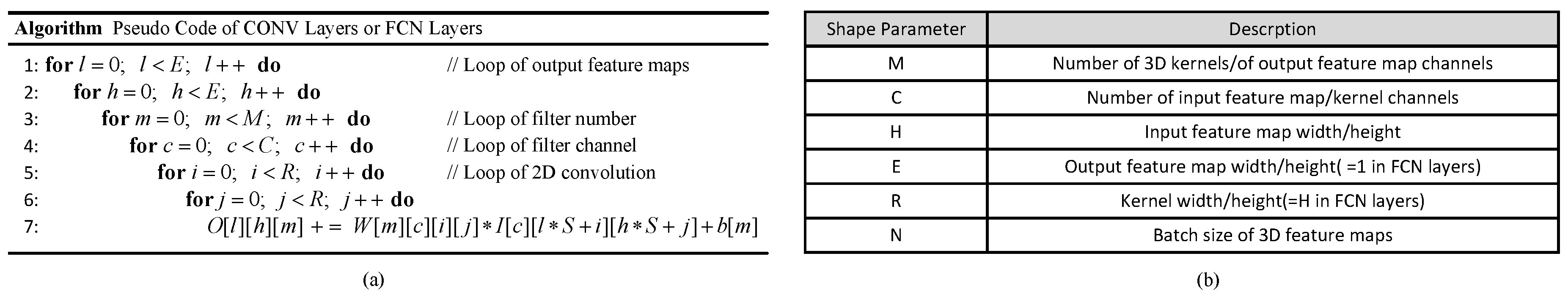
A CNN model essentially consists of cascaded layers, including the CONV layers, FCN layers, activation layers, pooling layers, and batch normalization layers. The CONV layers and FCN layers are the two most critical steps. The CONV layers bear the most intensive computation and apply the filters on the input feature maps to extract embedded visual characteristics and generate the output feature maps. For instance, it receives C input feature maps and outputs E output feature maps. The E output feature maps correspond to the filtered results of E 3-D filters. Each 3-D filter is operated on C input feature maps to generate one output feature map. The FCN layers are usually stacked behind the CONV layers as classifiers. The FCN layers mainly perform matrix multiplication. In FCN layers, the features can be represented as a vector, each node of this vector is connected to all nodes of the previous layer, which explains the huge amount of parameters and the requirement of high bandwidth. Figure 1a shows the computation loops of a single CONV or FCN layer. The descriptions of these parameters can be seen in Figure 1b.
However, the CONV and FCN layers are combinations of linear functions, which cannot generate new feature information. To tackle this problem, the CONV and FCN layers are usually followed by the activation layers. Its non-linearity brings in new characteristics. Popular activation functions include the hyperbolic tangent function and the rectified linear unit. Besides, the pooling layers, which execute a non-linear down-sampling function, also bring some new changes to the features. Generally, the max-pooling (MaxP) is the most popular choice, which outputs the maximum point from a small subregion of the feature maps [29]. The batch normalization layers make a difference in the process of training, and it can accelerate the convergence and avoid the overfitting problem. With the batch normalization layers [30], models can obtain the same accuracy with 14 times less training time. It can alleviate internal covariate shift by normalizing the inputs of layers.
We take a CONV-based layer block as an example. It includes a CONV layer, a batch normalization layer, an activation layer, and a MaxP layer. A typical process is
where l is the index of layers, a represents the input feature maps, b is the bias, y denotes the output feature maps.
2.2. Low Bit-Width CNNs
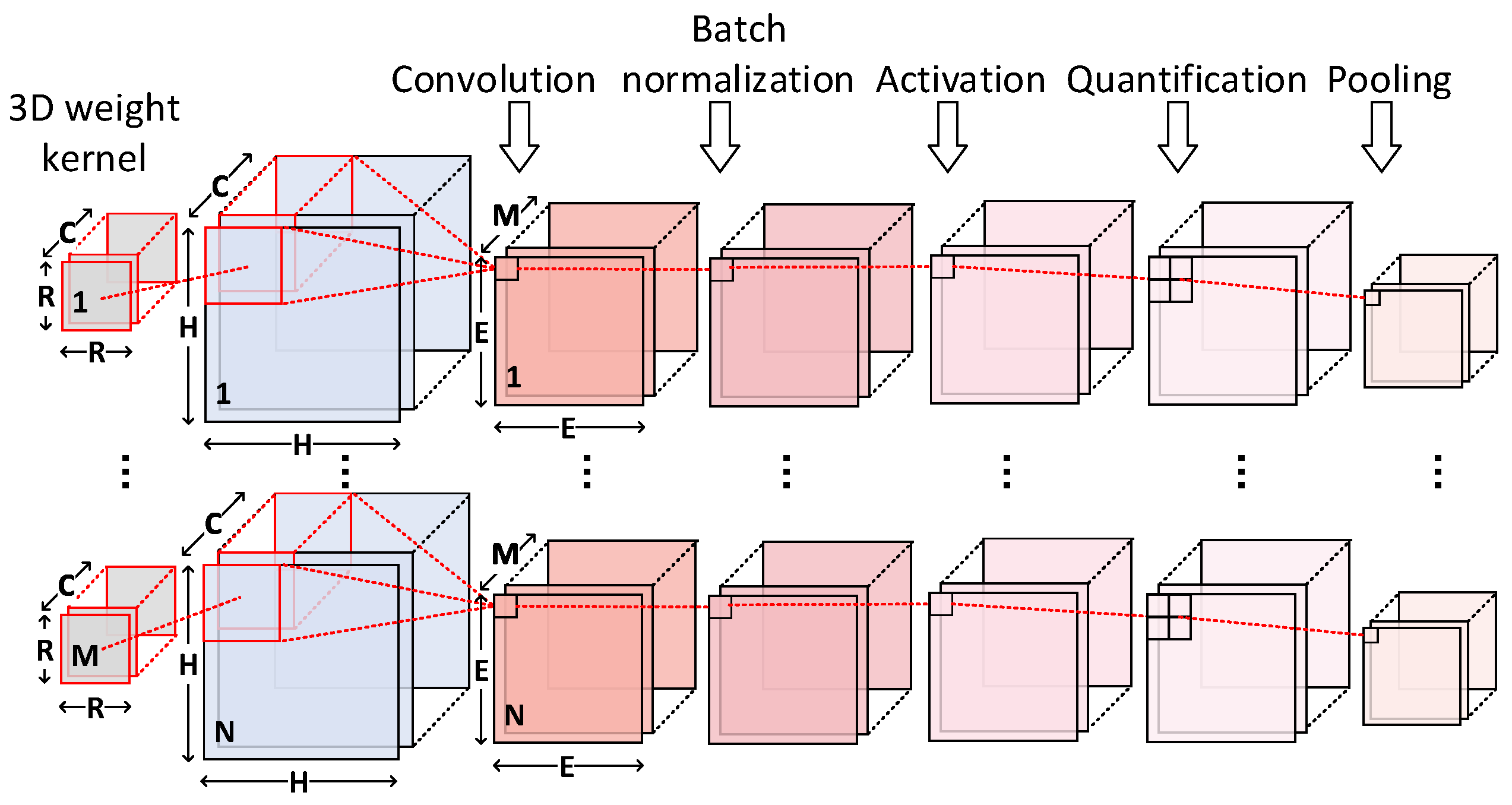
The low bit-width CNNs are similar to the conventional CNN models in terms of the structures. DoReFa-Net [11] is a method to train neural network that has low bit-width weights, activations with low bit-width parameter gradients. While weights and activations can be deterministically quantized, gradients are also stochastically quantized. AlexNet using the method of DoReFa-Net that has 1-bit weights, 2-bit activations, can be trained get 0.498 top-1 accuracy on ImageNet validation set, higher than BNN (0.279) and XNOR-Net (0.442). In this paper, the benchmarks and the algorithm refer to the DoReFa-Net. In the model DoReFa-Net [11], weights and activations are trained as k-bit and m-bit fixed-point integers respectively. As illustrated in Figure 2, within a CONV-based layer block, after convolution operations, there are four more steps we should take: batch normalization, activation, quantification, and optional max-pooling operations. The data of output feature maps after convolution are normalized by the trained statistical mean and variance . In addition, the results are processed by the scaling factor and the shifting parameter . The common simplified batch normalization can be regarded as a linear function. Thus
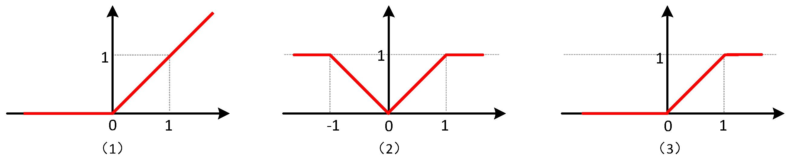
The activation operation is used to restrict the outputs ranging from zero to one. In this low bit-width CNN model, we can choose one of the following three kinds of activation functions, as shown in Figure 3, to add the non-linearity, thus
where is a function defined in Tensorflow, and will filter out the values beyond .
After that, the quantification function quantizes a real number output from the activation layers to a k-bit fixed-point number , which represents a few certain values.
At last, the max-pooling operation will be chosen optionally to reduce the size of the feature maps, thus
3. Efficient Parallel Streaming Architecture for Low Bit-Width CNNs
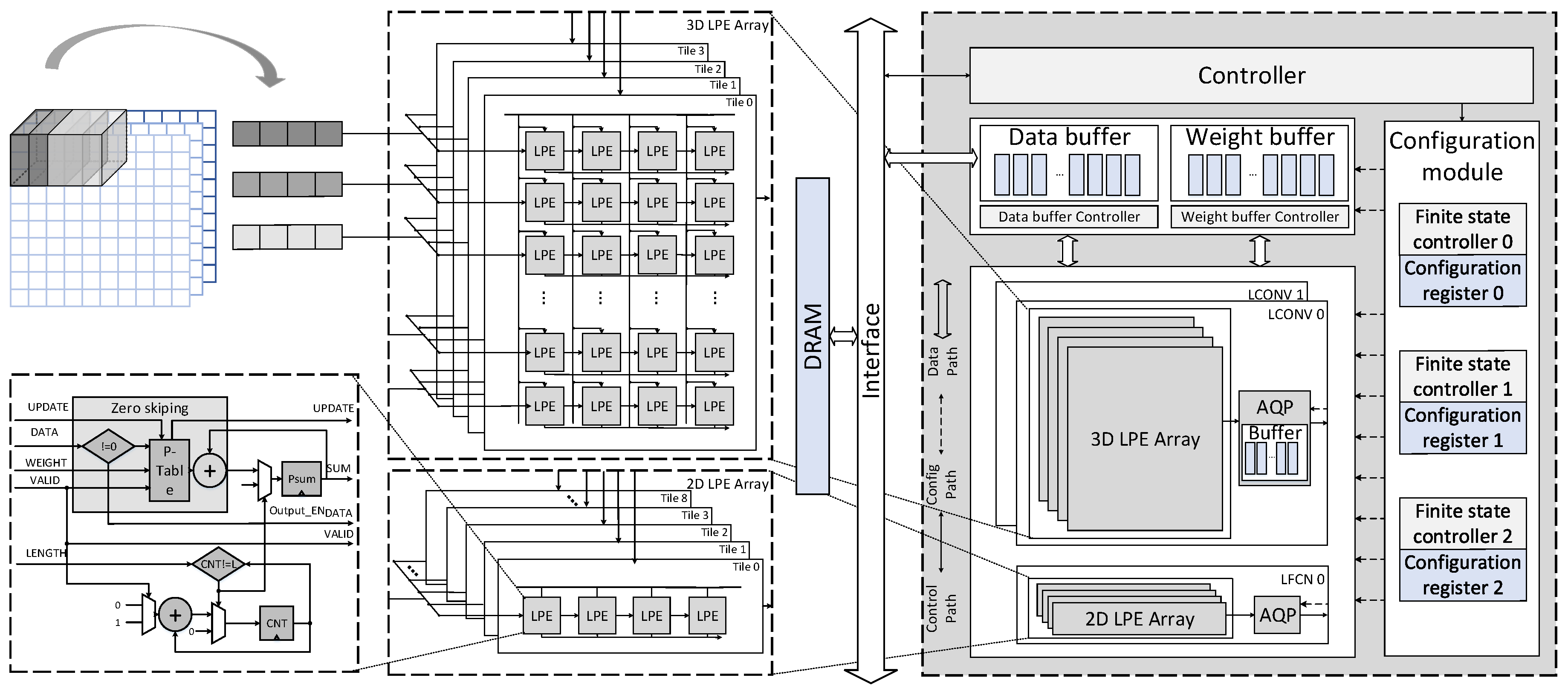
First, we describe the top architecture of this accelerator, as shown in Figure 4. Second, we describe the computing unit, which is the main component of this design, to introduce the novel dataflows and the CGTP strategy. Then the novel reconfigurable three-stage AQP unit is proposed, which is another important part of the computing unit. Finally, we describe the novel interleaving bank scheduling scheme.
3.1. Top Architecture
Figure 4 shows the overall architecture of the CNN accelerator. It is already proved that low bit-width neural network in [11] can also achieve competitive classification accuracy compared to 32-bit precision counterpart based on amounts of experiments. Besides, the properties of low bit-width provide more exploration space in terms of low power and high efficiency. In our work, we choose 2-bit and 1-bit as the data format of activations and weights respectively.
The accelerator is mainly composed of computing units, a memory module, a controller, and a configuration module. The computing units consist of three heterogeneous parts: two low bit-width convolutional computing (LCONV) units and a low bit-width fully connected computing (LFCN) unit for processing CONV-based layer blocks and FCN-based layer blocks, respectively. Each unit contains different subelements. For example, the LCONV unit is composed of a 3D systolic-like low bit-width processing element (LPE) array, and 16 activation, quantization and optional pooling (AQP) units. Compared to LCONV units, an LFCN unit is composed of a 2D systolic-like LPE array and an AQP unit. The dimension of computing array in CONV unit and LFC unit is 2 × 13 × 4 × 4 LPEs and 9 × 4 LPEs respectively, and the total number is 452 LPEs. The memory module includes a single port SRAM and an SRAM controller, which are both separated into the weight part and the input feature data part.
The overall execution is managed by the controller. The instructions, which can be categorized to execution and configuration, are fetched in the external memory via Advanced Extensive Interface (AXI) bus and decoded in the controller. The execution commands are responsible to initiate the execution. The configuration contexts, such as stride, number of channels, initial address and so on, are transferred to the configuration module. After receiving the configuration contexts, the configuration module reconfigures the data path, and the buffers supply data and parameters to computing units. These computing units are respectively controlled by separated configuration contexts and finite state controllers in the configuration module.
This parallel streaming architecture is very suitable for CNNs.
- (1)
- CNNs have cascaded layers, which can be executed as sequential modules.
- (2)
- multiple loops of intensive computation within a layer can be partitioned and executed in parallel conveniently.
- (3)
- the CNN accelerator should handle large batches of classification tasks based on the application requirements.
3.2. 3D Systolic-Like Array and Dataflow
3.2.1. Merging Bit-Wise Convolution and Batch Normalization into One Step
We combine the bit-wise convolution operation with the batch normalization, on account of their common linear characteristics. In this way, we can operate the CONV layers and batch normalization layers together without any latency, additional consumption or silicon area overhead.
The computation expression of the convolution is demonstrated in Figure 1. The batch normalization stacked behind will transform the expression linearly by factors of , , and , which can be formulated as (4). We merge the similar terms, thus
where p equals to , q equals to , and these two parameters can be pre-computed offline.
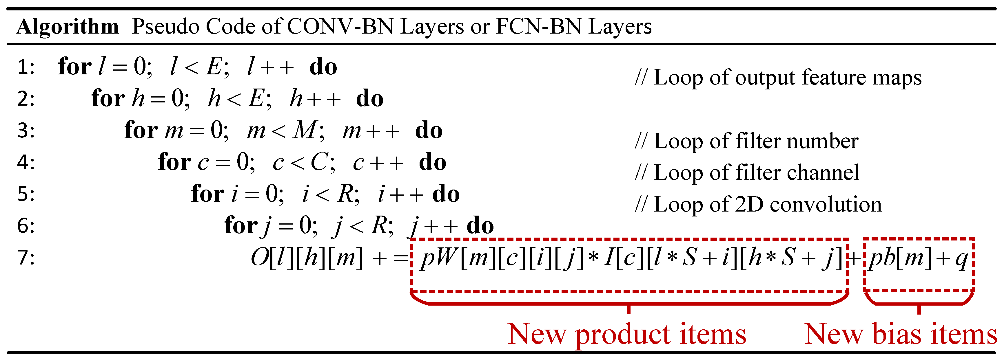
As shown in Figure 5, the results of the combination of CONV or FCN layers and batch normalization layers can be obtained by multiplying each product item with p and adding q to each bias item.
3.2.2. 3D Systolic-Like Array
In the original bit-wise convolution, the product of 1-bit weight and 2-bit activation has eight possible values. According to the optimized combination, we only need to change the pre-computed values stored in the local buffer and modify the bias values before parameters are sent to the weight buffers from the external memory. These additional operations will be finished offline, and operate without any overhead in hardware. Systolic arrays can date back to 1980s. However, history-aware architects could have a competitive edge [31]. In this work, we adopt the systolic array as our basic computing architecture. By the systolic dataflow, data can be continuously streamed along two dimensions of an array and processed in a pipelined fashion. When accelerating the CONV layers, we further improve data reuse by extending a conventional 2D array to a 3D tiled array for the intensive computation.
Figure 4 shows that a fixed number of rows are clustered to form a tile. Each tile has three groups of IO ports at the left, upper and bottom edges. The input feature data are loaded at the left edge and are horizontally shifted to the LPEs inside the tile on every cycle, weights are broadcasted to LPEs located in the same column. The outputs are locally generated on each LPE, and they are shifted to the edge of the array in the same direction with the input feature data. This dataflow is known as the output stationary defined in [19].
As shown in Figure 4, we introduce an LPE unit as the basic processing element, which executes local multiply accumulations. Besides, it also supports zero-skipping. An LPE unit mainly consists of a product table and an adder. The table can be updated by the same approach of transferring data in the array. The LPE can process one pair of the input feature data and weight at one cycle. In these trained models, the possibility that zeros occur among the values of activations is generally more than 30%. As known to all, multiplications with operand zero are ineffectual, besides, the zero products have no impact on the partial sum. In our design, multiplications with zero operands have been eliminated to reduce the power consumption.
3.2.3. Multi-Pattern Dataflow
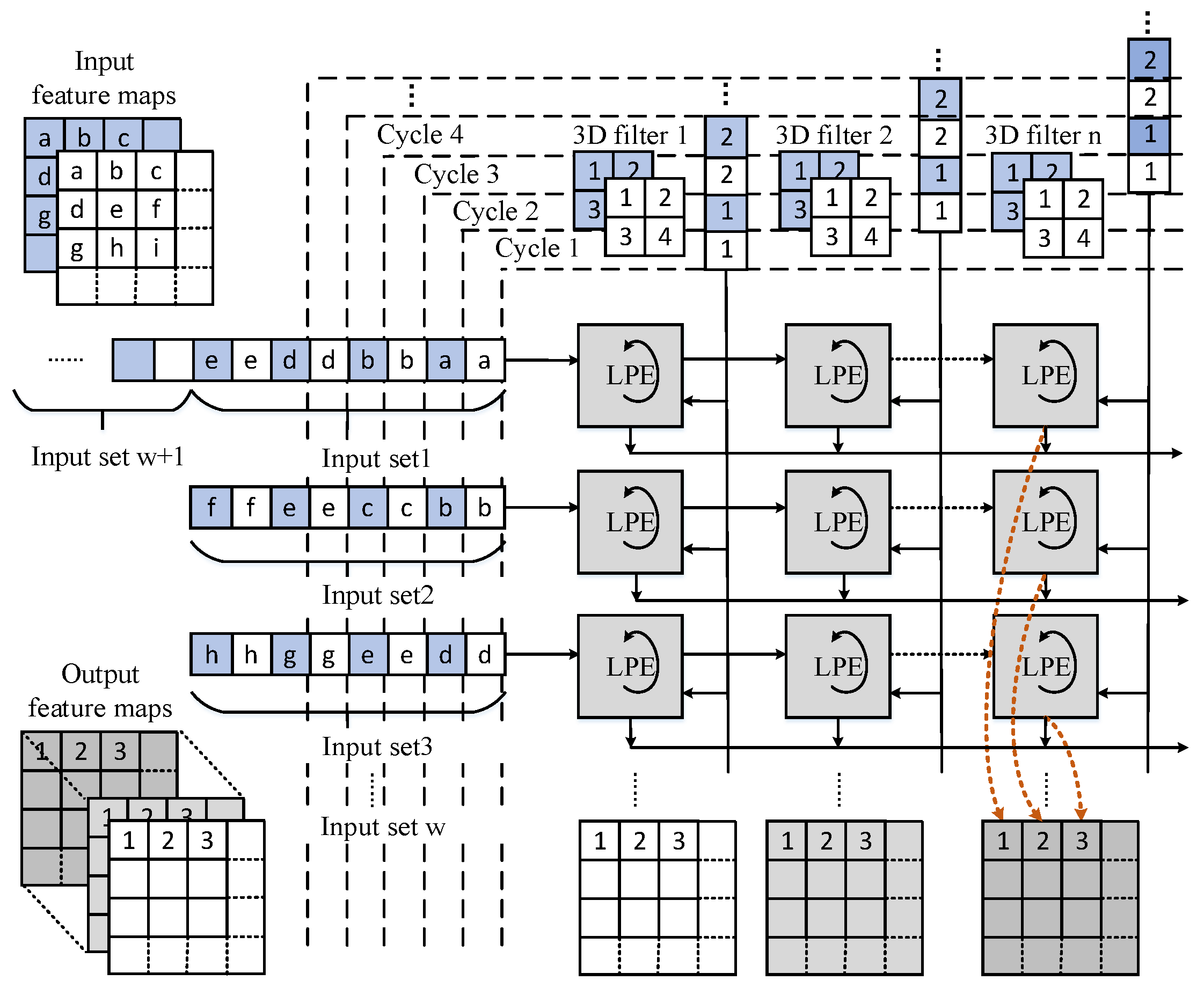
From an overall perspective, the input feature data are processed by three computing units one by one. In the LCONV units, the computing begins with feeding the input feature data and weights to the first 3D tiled systolic array LCONV0 for convolutional operations by the output stationary dataflow. In this way, inside a tile, as shown in Figure 6, the LPEs of the same column will generate output points located at one output feature map, whereas the output points computed in the LPEs of different columns are located at different output feature maps.
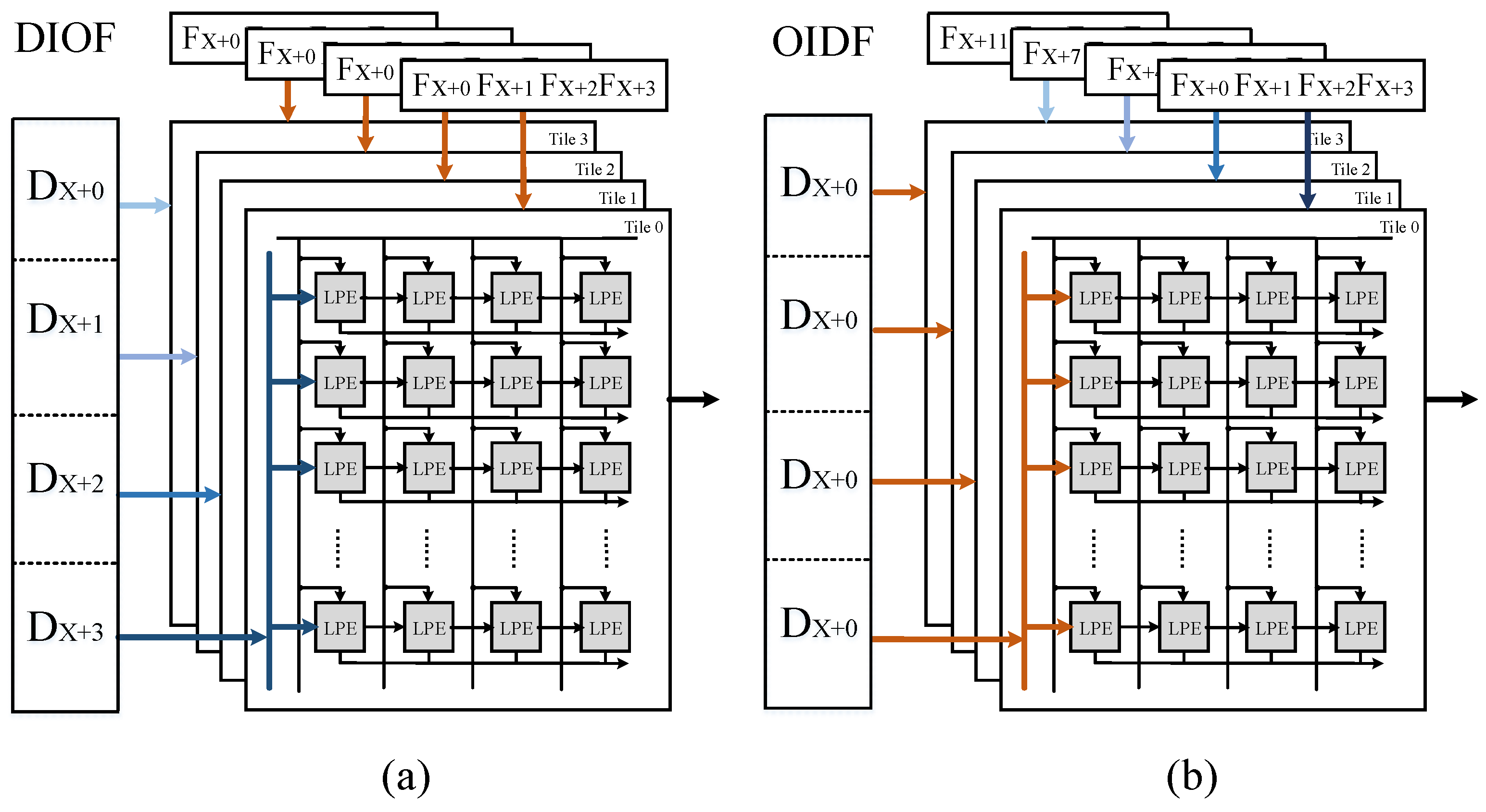
Each tile computes independently, but we can decide on the manner in which the data and weights are sent to the different tiles of the computing unit, depending on the configuration contexts, in order to improve the array use of the different sizes of CNNs. As depicted in Figure 7, one way is that tiles share one set of input feature maps but with different sets of filters (OIDF), another is that tiles load different input feature maps only with one set of filters (DIOF). If the number of filters is much larger than , we consider that the former dataflow is better. However, if the number of the filters is much less than , the second way should be selected to cater to the less-filters CONV layers.
This architecture is flexible to be used with any size of images and also any size of convolution kernel (e.g., , , , …), because of the dataflow inside a tile which gives the priority to data along the channel in the input feature maps. However, the stride does have a limitation, which cannot be over 4, due to the bandwidth limitation of SRAM.
3.3. Coarse Grain Task Partitioning Strategy
Tasks can be partitioned and allocated to several computing units in coarse or fine granularity. The coarse grain indicates that the partition works on the inter-layer level, while fine grain refers to partition works on the intra-layer level. Compared to the fine granularity, the coarse granularity partitioning can reduce the communication overheads between computing units, and avoid much control and configuration logic. Our design regards one layer processing as the minimum task, which cannot be further divided.
If tasks are not well partitioned, they will introduce the large load imbalance. The computing units holding easy tasks will be compelled to wait for the units bearing heavy tasks. Thus, the slowest computing unit will dominate the throughput. To address this problem, the coarse grain task partitioning (CGTP) strategy is proposed to keep the loads of two LCONV units as balanced as possible. The CONV and FCN layers contribute to almost all the computations and storage of CNNs, whereas other layers can be omitted. The FCN layers can be regarded as CONV layers when the size of input feature maps and filters are the same. Due to the limited hardware resources, it is necessary to unroll the loops and parallelize the low bit-width CNNs onto our existing hardware with a certain number of iterations [32]. Suppose the size of computing array is . Accordingly, the parallelism should be . The computing cycles of a single CONV layer is divided into two kinds, one is the OIDF dataflow case:
and another is the DIOF dataflow case:
In addition, as for FCN layers, the computing cycles can be calculated by the following formula:
In our design, the layers of a CNN model are separated into three groups, which correspond to three tasks. Each group of layers will be mapped into one computing unit. In this work, we allocate an independent computing unit LFCN0 for FCN layers due to its low parallelism. Thus the problem is simplified into dividing CONV layers into two groups. Hence, we design Algorithm 1 to obtain two groups with the roughly equal runtime. Firstly, we get the whole processing time of a CNN model from the first loop computing. Secondly, during each pass in the second loop, it adds the processing time of each CONV layer one by one iteratively, and store the current and the last accumulated time. Then a series of comparisons will be made among these values to decide which group the current CONV layer should join.
| Algorithm 1 Coarse Grain Task Partitioning |
| Input: Number of CONV layers L; detailed dimensions of each CONV layer ; detailed dimensions of LCONV ; dataflow mode Output: Two groups
|
3.4. Reconfigurable Three-Stage AQP Unit
3.4.1. Modified Quantification
The layers of activation, quantification, and optional pooling can also be adjusted by some transformations to simplify the executing process. For example, Equation (6) shows that the outputs from CONV or FCN layers will be activated by taking the minimum between the absolute value of the inputs and 1, which can restrict the value to [0,1] to meet the requirement of the input range for the quantification step. As for the quantification, it is demonstrated in (8) that the outputs will be quantized to four possible values under the case of 2-bit quantification (). It can be implemented by a series of comparisons between the outputs of activation layers and the thresholds of . For example, a certain output neuron equals to , which is bigger than whereas smaller than , therefore, it will be quantized to . We make some adjustment to the original quantification function (8). The modified function is shown below, which mainly changes the function :
where x represents the absolute value of the output point from CONV or FCN layers.
The modified quantification function will no longer be limited by the input range obtained by the activation, because this modified version has already taken those inputs out of the range into account. It can achieve the same effect with the previous activation and quantification functions. Besides, this modified quantification function also applies for the second activation function (7) where x denotes the output point from CONV or FCN layers.
3.4.2. Architecture of AQP Unit and Dataflow
The MaxP layers has the similar computing pattern with the modified quantification layers mentioned above. Moreover, the max-pooling operation does not always exist in every CONV-based layers block. Therefore, it is not efficient to allocate an independent piece of hardware for it. Hence, we propose an efficient reconfigurable three-stage AQP unit, which can be reconfigured to two modes: activation-quantification-pooling (AQP) mode and activation-quantification (AQ) mode. Thanks to the design of the AQP unit, the max-pooling operation can be incorporated in the process of the activation and quantification at the hardware level, which means that processing max-pooling operations will not bring any overhead. Besides, the design can be further optimized to be more energy-saving with the staged blocking strategy. Moreover, the three-stage pipeline structure can reduce the data path delay and support flexible window size.
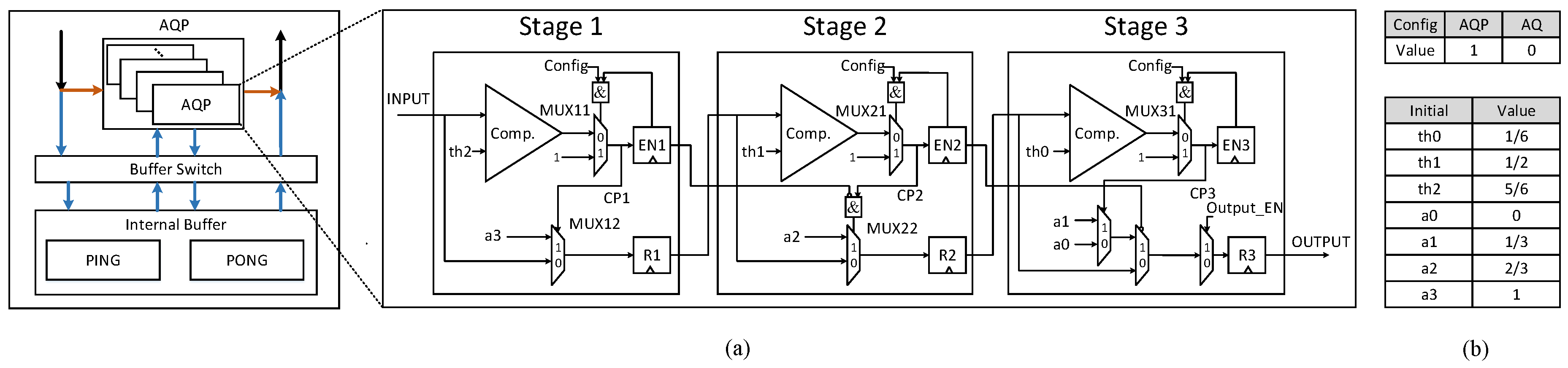
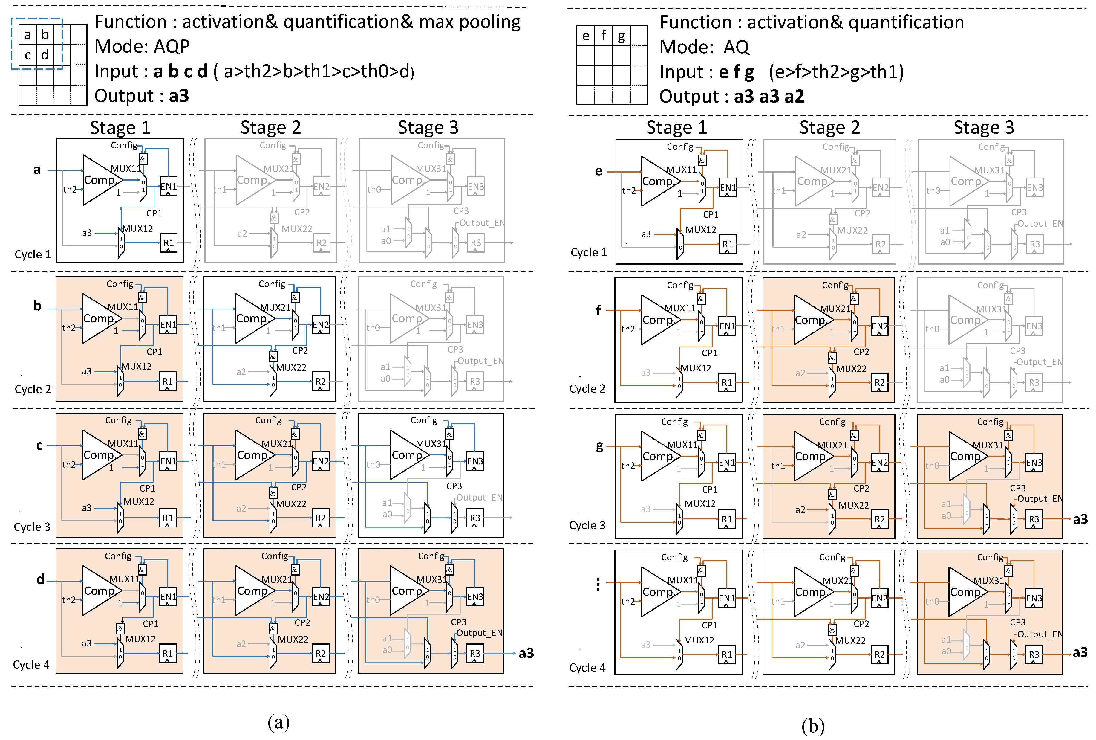
As shown in Figure 8a, its function is controlled by a 1-bit configuration word , which 1 denotes AQP function and 0 represents AQ function. The AQP unit is composed of three stages, each stage primarily comprises a comparator and some registers. The three-stage structure enables it to work in a pipelining way, which allows for supporting the different sizes of the max-pooling window.
As depicted in Figure 8, the AQP module is designed as a separate part of the computing units, which mainly consists of the AQP units and the internal buffer. When is set as AQP mode, it fetches the output feature data stored in the Ping-Pong internal buffers, which can ensure that the convolutional and AQP operation will not interfere with each other and can be processed simultaneously. Furthermore, the convolutional operation is far more computing intensive than the max-pooling operations. Therefore, the convolution can be processed in a non-stop way. When the dataflow in the 3D systolic-like array is OIDF, it will generate a portion of the data located at 16 output feature maps simultaneously over a period of continuous time. Each of 16 output feature maps has its own bank group to guarantee that data points of each output feature map can be accessed at the same time. When the dataflow in the array is DIOF, the array will produce part of data located at 4 output feature maps for a continuous period of time. In this way, every four AQP units will process data of one output feature map. When is set as AQ mode, the data will stream into the AQP units directly without waiting in the internal buffers. There are 16 AQP units in each LCONV, and there is only one in LFC computing array.
3.4.3. Working Process of AQP Unit under Two Modes and Staged Blocking Strategy
The comparator will output positive when the operand above is bigger than the operand below. Figure 9a shows the details of the processing in AQP mode, and the is set as 1. For example, assumes that are four pixels of a subregion from one feature map, the value relationship among these pixels and thresholds is: . These four pixels enter the AQP unit one by one. At the cycle 1, the pixel a compares with , since a is bigger than , the comparison signal turns to 1 and stored in the register . Therefore, is chosen as the quantification result of a, stored in the register in the stage 1. At the cycle 2, the pixel b enters the stage 1 of the AQP unit, for the register has already been set as 1 at the previous cycle, whatever the relationship of b and , the comparison signal should be kept at 1 controlled by . Therefore, the register remains unchanged. At the same time, in the register passes to stage 2 and compares with . Although is larger than , the signal still remains 0 controlled by the passed from stage 1, therefore, the output will be kept at . In this way, the register will keep the first comparison result , and so on. Once the signal turns to 1, the result stored in the register will be sent out.
It means that if the input is bigger than the threshold at a certain stage, the register will turn to 1 to shut down the rest operations in both horizontal (the remaining pixels streaming in) and vertical (the remaining stages processing the current pixel) direction within the subregion to reduce high-low or low-high transitions.
Figure 9b depicts the details of the processing in AQ mode, the configuration word is set as 0, it means that the comparison signal will no longer be influenced by of the local stage at the previous cycle, but it will still be controlled by of the previous stage at the previous cycle. It means the set of registers will hold back the rest operations vertically. In one sense, the register works like a gate to block the useless operations. Due to less switching, a significant reduction in power consumption can be created.
3.5. Interleaving Bank Scheduling Scheme
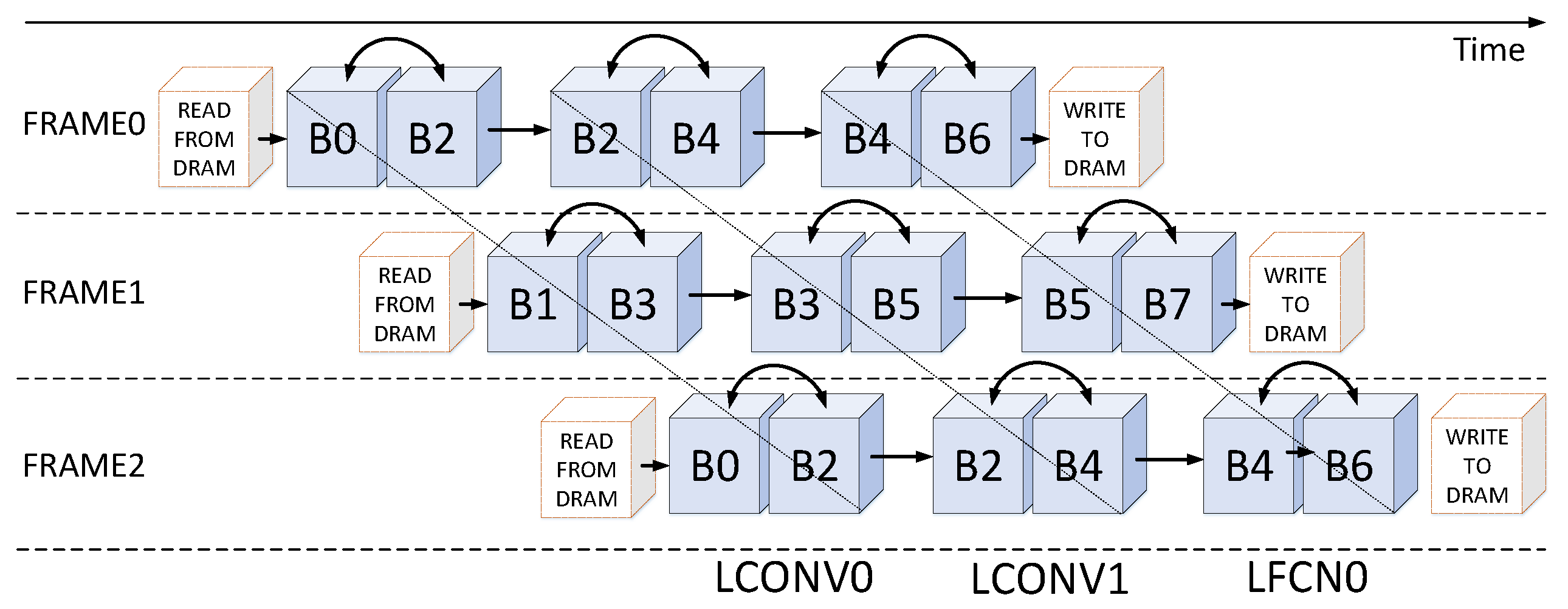
In order to guarantee the conflict-free data accesses and improve memory resource efficiency, an interleaving bank scheduling scheme is proposed. Algorithm 2 depicts the details. Figure 10 shows one of the situations of the algorithm. We can observe that the multi-bank memory module can be divided at two levels:
- Frame Level: the bank group 0 and the bank group 1 are loaded input feature maps of different frames from external memory alternatively. This means that all even-numbered bank groups are configured to provide and receive data on one frame, and all odd-numbered bank groups support another frame.
- Computing Unit Level: each computing unit corresponds to a specific set of bank groups, for example, the LCONV0 and the LCONV1 connect to the bank group 0–3 and the bank group 2–5, respectively, the LCFN0 links to the bank group 4–7.
| Algorithm 2 Interleaving Bank Scheduling Scheme |
|
If the data of input feature maps is more than capacity of SRAM, the feature maps will be divided according to its row instead of the channel. Within the bank group (e.g., B0-7), there is a Ping-Pong strategy working for transferring the intermediate outputs to the external memory when the capacity of SRAM is not enough for a certain network. So actually, there is no limitation on the input size because you can always divide the input feature maps if it is too large. For example, when processing the small network like S-Net which is derived from Dorefa-net, there is no need to cache for multiple times. Besides, the time transferring data from DRAM to SRAM can be covered by computation.
Our design has two single-port SRAM, one for the data buffer and the other for the weight buffer. The data buffer is composed of 14 banks, the weight buffer is composed of 6 banks. In the data buffer, 14 banks are partitioned into 4 groups: 4-bank, 4-bank, 4-bank, 2-bank. The first three is designed for supporting the CONV layers under the streaming architecture with Ping-Pong manner. The last one is to support the FCN layers, considering that it is the last step of CNNs processing, 2 banks are enough. In the weight buffer, 6 banks are partitioned into three 2- bank groups. Each group is used to provide weights to three computing units (two LCONV units and one LFCN unit). The capacity of the data buffer is KB. The total bandwidth of each bank group is set as 104-bit, which can support the maximum stride of 4. The weight buffer is KB, and the pooling buffer is KB, which is sufficient to store the intermediate feature data.
4. Evaluation
In the evaluations, four networks AlexNet, VGG-16, D-Net and S-Net (SVHN-based CNN models) are chosen as benchmarks. These models are derived from DoReFa-Net proposed in [11], which weights and activations are represented by 1-bit and 2-bit respectively. First, the combined performance of different task partitioning strategies and dataflows will be evaluated with the four benchmarks. Then the comparison with some state-of-the-art designs is shown.
4.1. Evaluation Metrics
4.1.1. Computation Complexity
The total number of both additions and multiplications are taken into account according to Diannao [33]. In this way, the number of operations can be calculated as follows:
due to the optimization above, the operations of batch normalization is hidden in the convolutional operation, which requires no extra calculation.
4.1.2. Performance
It means that the reachable throughput of a system can be calculated theoretically as follows:
where l denotes the number of the computing units and f represents the frequency. However, we cannot make the computing unit at full load all the time mainly for irregularly shaped networks. Therefore, we calculate the effective throughput as follows:
where s represent the number of layers within each group after the task partitioning, T is the interval (i.e., the processing time of the slowest computing units). Besides, there are still two metrics to evaluate the efficiency, the energy efficiency is
the area efficiency is
In addition, the use of arithmetic units is noteworthy, thus
4.2. Performance Comparison
We firstly design a cycle accurate behavior model using SystemC language for the whole system, including the accelerator, the AXI interface, DMA and DRAM, to simulate and verify the data path, the control path, and the configuration path. Then the design is coded in register transfer level (RTL) and synthesized with TSMC 40 nm technology with Synopsys Design Compiler. The peak performance is GOPS, the core power is mW at 800 MHz frequency. According to DoReFa-Net [11], the series of CNNs with 1-bit weight and 2-bit activation also have competitive accuracy.
4.2.1. Analysis on CGTP Strategy
The recent work of [21] partitions PE arrays into several parts, whereas only one block of the PE array is allocated to process CONV layers. The difference is that we design double processing units for the CONV layers and take the CGTP strategy to balance computing load and obtain minimal execution time. Without CGTP strategy, the processing time of CONV layers is much longer than that of the FCN layers, and this unbalance will lead to the long pipeline stalls and low throughput. We set the approach of [21] as a baseline, and compare the performance and array use between it and this work using the four benchmarks.
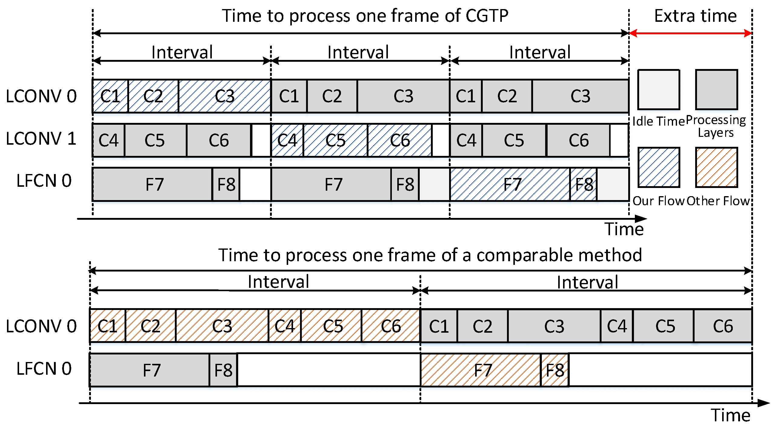
Figure 11 illustrates the comparison based on the D-Net model. Table 1 shows the D-Net model architecture. The blue-slash background grids indicate an example of processing a complete model in our design, which spans three short intervals, whereas the red-slash represent that of [21], which spans two long intervals. The white background grids show the suspension of computing units, which is caused by the different processing time of these computing units. We can observe that the idle time is less in our design. Thus the time to process one frame is shorter. Besides, the data dependencies between neighboring layers are allowed, which can remove some unnecessary data movement. As shown in Figure 12, the throughput and the array use are greatly improved by nearly due to the CGTP strategy on average.
4.2.2. Analysis on Dataflow
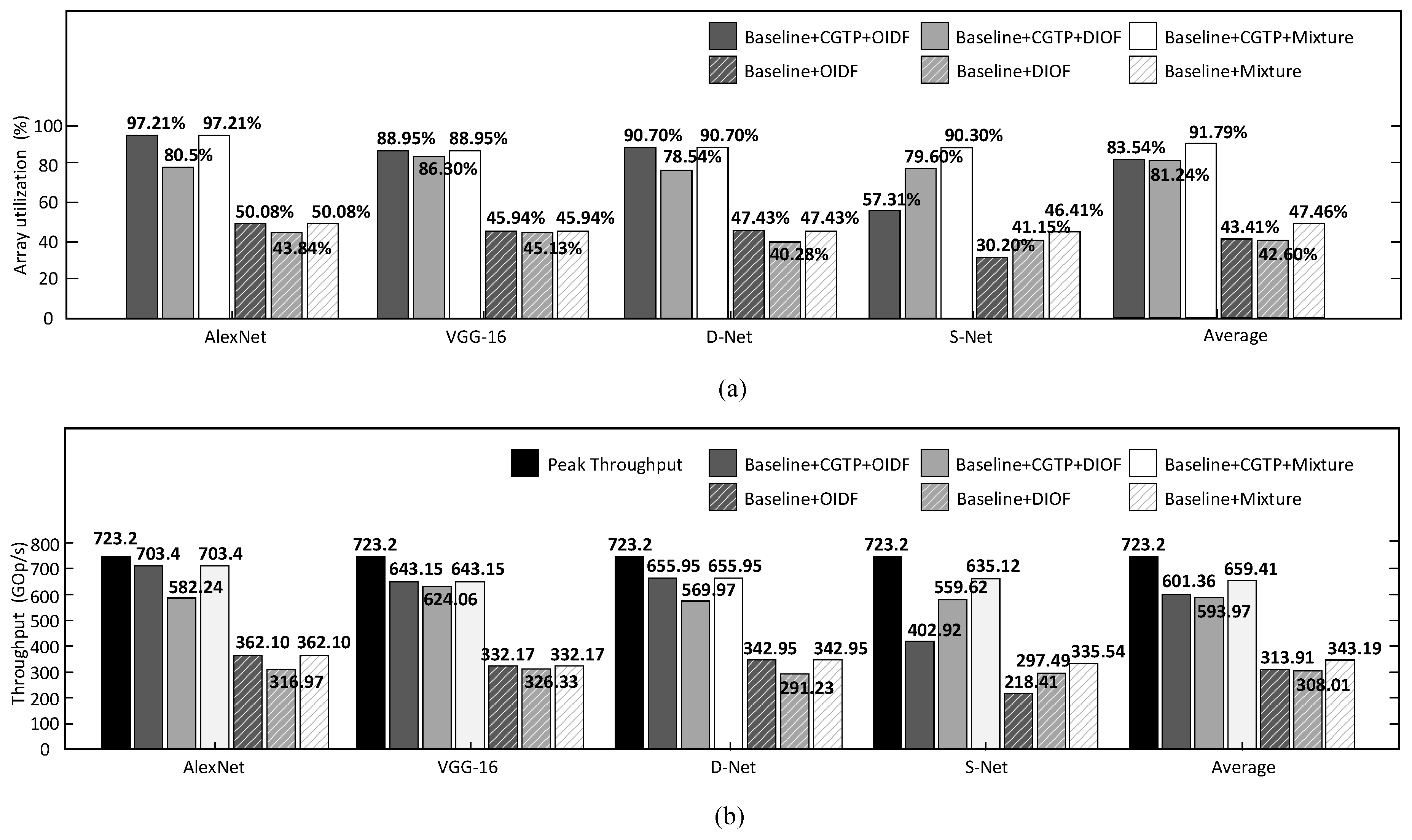
In the processing of the CONV layers, we introduce three kinds of the dataflow: OIDF dataflow, DIOF dataflow, and their mixture, which apply to three kinds of CNN models, respectively. The OIDF dataflow is more suitable for the CNN models with a great number of filters at each layer, whereas the DIOF dataflow is designed for the CNN models consisting of less-filter layers. As for the third kind of CNN models, there are not many filters at the former layers, but the number will increase as going deeper. In such situations, the mixture dataflow is more appropriate. In general, the first and the third kind of CNN models are more popular. Figure 12 shows the comparison between these three kinds of datalows on four benchmarks after the CGTP optimization. Besides, we describe the task partitioning approach for each benchmark under every dataflow in a very detailed manner, as shown in Table 2. It is observed that the specific partition approach will change with the dataflow, due to the different processing time of each layer under different dataflows. For instance, when the benchmark is AlexNet, the LCONV1 unit will process the CONV1 and CONV2 layers, and the LCONV2 will process the CONV 3–5 layers under the DIOF dataflow.
Each layer of both AlexNet and VGG-16 have a relatively large number of filters, so does D-Net. So the throughput and array use are the same high when adopting the OIDF dataflow and the mixture, whereas becoming lower with the DIOF dataflow. S-Net is a typical example of the third kind of CNN models, which is derived from Model D-Net by reducing the number of filters for all the CONV layers and the first FCN layer by 75%. S-Net has only about 3% degradation in top-5 accuracy, whereas the number of parameters largely decreases, compared to D-Net. In the test case of S-Net, we notice that about 30% degradation in the throughput and array use when adopting the OIDF dataflow compared to the DIOF dataflow. It is also observed that S-Net applied with the mixture dataflow can get nearly double performance compared to the OIDF dataflow.
Among these benchmarks, it is shown that this work can achieve GOPS throughput and % array use on average. Moreover, we can observe that AlexNet, which has the biggest ratio between the computation loads of FCN layers and the computation loads of CONV layers among those benchmarks, shows the best performance with GOPS. The reason is that when we allocate the relative number of LPEs for the CONV and LFC units, we give the priority to AlexNet because it has the heaviest computation loads of FCN layers. If we increase the ratio of the LPE number of the LCONV units and LFCN units, the processing time of the LFCN unit will be much longer than the other two units due to less LPEs in AlexNet. So, to some extent, AlexNet is the bottleneck of these benchmarks. As shown in Table 3, the resource use of LFCN unit is close to 100%. Besides, the performance of other three benchmarks are also about 90%, achieving great performance than previous works.
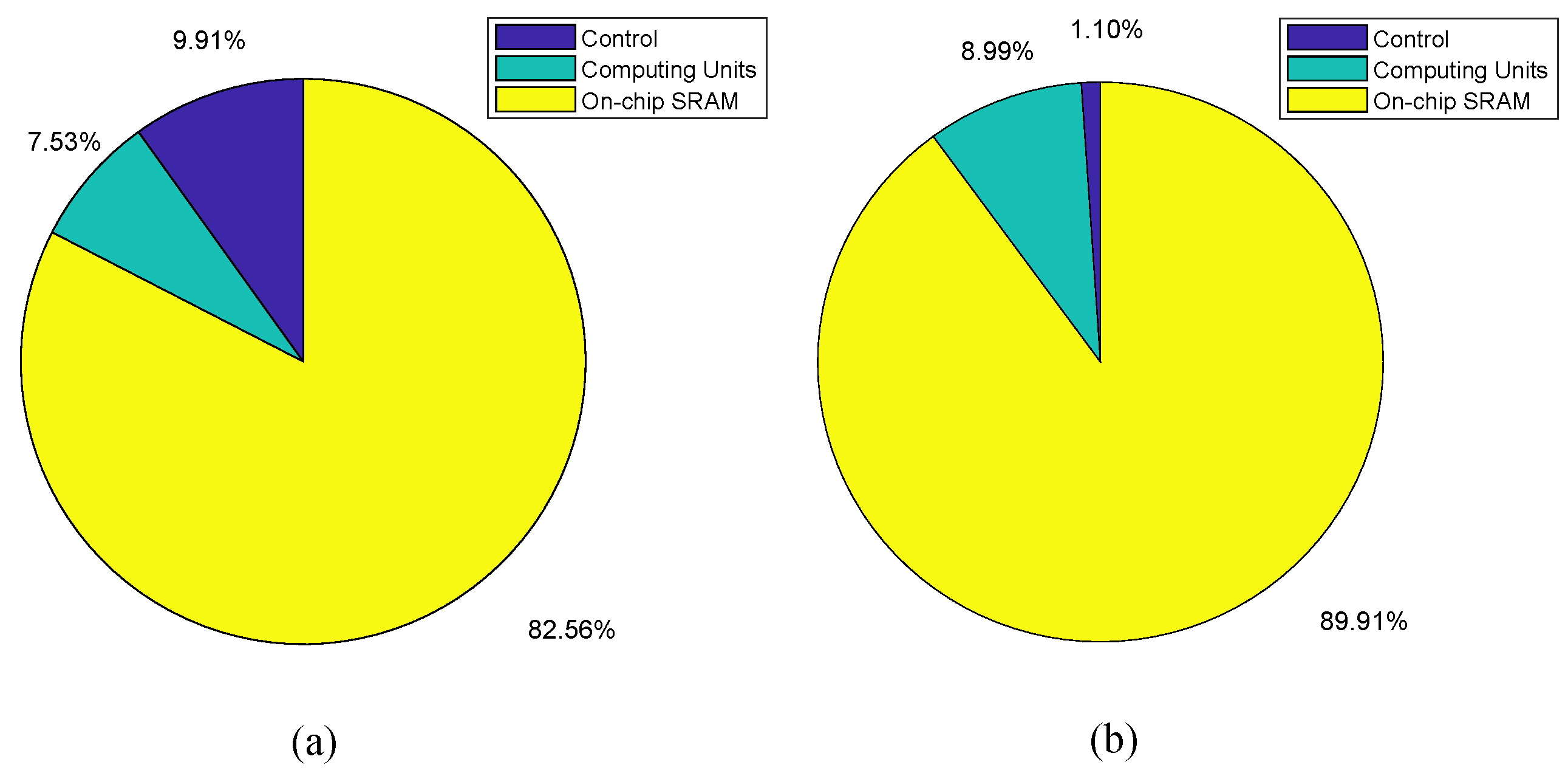
4.2.3. Synthesis Results of the Breakdown
The accelerator is composed of control modules (controller and configuration module), computing units, and on-chip buffers. We have synthesized the three parts with Synopsys Design Compiler respectively, and the power/area breakdown of the accelerator has been illustrated in Figure 13 in the revised version. The area and power breakdown are calculated based on the Synopsys Design Compiler. The logic module takes 9.91% area and 1.10% power. The computing units take 7.53% area and 8.99% power. The memory consumes 82.56% area and 89.91% power to store and transmit the weights, activations and integral values.
4.2.4. Comparison with Previous Works
Some research, like that in [21,34], usually cannot make full use of the arithmetic units due to the shallow channels or the various sizes of kernels. For example, in [34], the convolution unit engine is designed according to the normal size of 3 × 3 kernel, which will lead to heavy underuse when processing other window size convolution, especially 1 × 1 convolution. Table 4 shows the details of processing the benchmark AlexNet, including the layer description, the latency, the interval, and the effective throughput. It is noted that the latency of each layer scales linearly with the number of operations in our design, which indicates our architecture and dataflow can well solve the problem and improve the array use at each layer. When accelerating AlexNet, it only requires ms to classify an image, achieving the TOP1 accuracy of .
Considering that those works like Eyeriss [15] and Diannao [33] are targeted at conventional CNNs with high precision are more complicated in computation, we only compare our work with low bit-width CNN accelerators. In order to make our design with 40 nm technology comparable with others, we follow a series of equations according to [17,35]. This projection gives an idea of how the various implementations perform in a recent technology.
where s denotes the scaling factor, l represents the channel length, f denotes the frequency, S denotes area, is the power supply voltage, P represents the power consumption. The dynamic power is caused by charging and discharging capacitances during switching, given by
where C is the switched capacitance, and A represents the switching activity factor. When our design scaled to 65 nm, the s equals to , the area changes from mm with 40 nm to mm with 65 nm technology, and the frequency is scaled to 492 MHz. To obtain the operating voltage in 65 nm technology, we set it as the common operating voltage of the used technology [17]. In addition, the result of power consumption, according to Equations (21)–(23), will be mW.
As shown in Table 5, our design has the highest area efficiency among these works. The QUEST [36], with a large 3D memory to store data on-chip, can achieve TOPS/W for (1,1)b AlexNet at 300 MHz and V. When comparing with QUEST, the energy efficiency of our work is about higher. YodaNN can achieve TOPS/W when supporting (1,12)b AlexNet at 480 MHz and V. BCNN, introducing optimized compressor trees and approximate binary multipliers, can achieve an energy efficiency over TOPS/W at 380 MHz and V. When comparing with YodaNN and BCNN, we scale our work to 65 nm technology, the results show that the energy efficiency of the proposed architecture is about and higher that of YodaNN and BCNN, but the area efficiency is about and higher. Furthermore, the area of this design is only mm, which is the smallest among the previous works. The on-chip buffer of QUEST and BCNN are both very large, which can reduce data accesses when processing large models. However, the cost is too large for relatively small models. Besides, BCNN and YodaNN do not take FCN layers into account, whereas this work can support the whole low bit-width CNN model acceleration.
It should be mentioned that such high efficiency can be attributed to various architectural level and algorithm level optimizations, detailed reasons can be listed as follows.
- The parallel streaming architecture with heterogeneous computing units can efficiently exploit the use of computing resources. Also, the CGTP strategy and the multi-pattern dataflow contribute a lot to improve the throughput respectively.
- The computing array cannot only execute the convolution or inner-product but also the batch-normalization function. Besides, the LPE is only composed of some “look-up table” registers, an adder and some logical registers.
- The AQP unit is only composed of comparators and registers. The function of activation, quantification and pooling can be implemented on the same piece of hardware simultaneously. Besides, the low power property is also exploited by the staged blocking strategy.
5. Conclusions
In this paper, we propose an efficient scalable accelerator for low bit-width CNNs based on a parallel streaming architecture. The proposed accelerator can optimize various sizes of CNN models with high throughput by applying the CGTP strategy, which is based on the heterogeneous computing units and multi-pattern dataflows. Besides, modified activation and quantification process is introduced to reduce redundancy of the computation. In addition, an efficient reconfigurable AQP unit is designed to support activation, quantification and pooling operations. Moreover, an interleaving memory scheduling scheme is proposed to well support the streaming architecture and reduce area overhead. The accelerator is implemented with TSMC 40 nm technology with a core size of mm. The result shows that this accelerator can achieve TOPS/W energy efficiency and about TOPS/mm area efficiency, making it promising to be integrated with the embedded IoT devices.
Author Contributions
Conceptualization, Q.C. and L.L.; methodology, Q.C.; software, Q.C.; validation, W.S., K.C.; formal analysis, Q.C.; investigation, Y.F.; resources, L.L.; data curation, W.S.; writing—original draft preparation, Q.C.; writing—review and editing, Z.L., C.Z.; visualization, Q.C.; supervision, L.L.; project administration, L.L.; funding acquisition, L.L., Y.F.
Funding
This research received no external funding.
Acknowledgments
This work was supported by the National Nature Science Foundation of China under Grant No. 61176024; The project on the Integration of Industry, Education and Research of Jiangsu Province BY2015069-05; The project Funded by the Priority Academic Program Development of Jiangsu Higher Education Institutions (PAPD); Collaborative Innovation Center of Solid-State Lighting and Energy-Saving Electronics; and the Fundamental Research Funds for the Central Universities.
Conflicts of Interest
The authors declare no conflict of interest.
References
- Tang, Z.L.; Li, S.M.; Yu, L.J. Implementation of Deep Learning-Based Automatic Modulation Classifier on FPGA SDR Platform. Electronics 2018, 7, 122. [Google Scholar] [CrossRef]
- Wang, X.; Hua, X.; Xiao, F.; Li, Y.; Hu, X.; Sun, P. Multi-Object Detection in Traffic Scenes Based on Improved SSD. Electronics 2018, 7, 302. [Google Scholar] [CrossRef]
- Liu, X.; Tao, Y.; Jing, L. Real-Time Ground Vehicle Detection in Aerial Infrared Imagery Based on Convolutional Neural Network. Electronics 2018, 7, 78. [Google Scholar] [CrossRef]
- Krizhevsky, A.; Sutskever, I.; Hinton, G.E. ImageNet classification with deep convolutional neural networks. Proceedinds of the Advances in Neural Information Processing Systems 25 (NIPS 2012), Lake Tahoe, NV, USA, 3–6 December 2012; pp. 1097–1105. [Google Scholar]
- Hannun, A.; Case, C.; Casper, J.; Catanzaro, B.; Diamos, G.; Elsen, E.; Prenger, R.; Satheesh, S.; Sengupta, S.; Coates, A.; et al. Deep Speech: Scaling up end-to-end speech recognition. arXiv, 2014; arXiv:1412.5567. [Google Scholar]
- Collobert, R.; Weston, J.; Karlen, M.; Kavukcuoglu, K.; Kuksa, P. Natural Language Processing (Almost) from Scratch. J. Mach. Learn. Res. 2011, 12, 2493–2537. [Google Scholar]
- Szegedy, C.; Liu, W.; Jia, Y.; Sermanet, P.; Reed, S.; Anguelov, D.; Erhan, D.; Vanhoucke, V.; Rabinovich, A. Going deeper with convolutions. In Proceedings of the IEEE Conference on Computer Vision and Pattern Recognition (CVPR), Boston, MA, USA, 7–12 June 2015; pp. 1–9. [Google Scholar]
- Han, S.; Mao, H.; Dally, W.J. Deep Compression: Compressing Deep Neural Networks with Pruning, Trained Quantization and Huffman Coding. Fiber 2015, 56, 3–7. [Google Scholar]
- Courbariaux, M.; Hubara, I.; Soudry, D.; El-Yaniv, R.; Bengio, Y. Binarized Neural Networks: Training Deep Neural Networks with Weights and Activations Constrained to +1 or −1. arXiv, 2016; arXiv:1602.02830. [Google Scholar]
- Rastegari, M.; Ordonez, V.; Redmon, J.; Farhadi, A. XNOR-Net: ImageNet Classification Using Binary Convolutional Neural Networks. In Proceedings of the ECCV, Amsterdam, The Netherlands, 11–14 October 2016; pp. 525–542. [Google Scholar]
- Zhou, S.; Wu, Y.; Ni, Z.; Zhou, X.; Wen, H.; Zou, Y. DoReFa-Net: Training Low Bitwidth Convolutional Neural Networks with Low Bitwidth Gradients. arXiv, 2016; arXiv:1606.06160. [Google Scholar]
- Jouppi, N.P.; Young, C.; Patil, N.; Patterson, D.; Agrawal, G.; Bajwa, R.; Bates, S.; Bhatia, S.; Boden, N.; Borchers, A.; et al. In-datacenter performance analysis of a tensor processing unit. In Proceedings of the 2017 ACM/IEEE 44th Annual International Symposium on Computer Architecture (ISCA), Toronto, ON, Canada, 24–28 June 2017; pp. 1–12. [Google Scholar]
- Qiu, J.; Wang, J.; Yao, S.; Guo, K.; Li, B.; Zhou, E.; Yu, J.; Tang, T.; Xu, N.; Song, S.; et al. Going Deeper with Embedded FPGA Platform for Convolutional Neural Network. In Proceedings of the ACM FPGA, Monterey, CA, USA, 21–23 February 2016; pp. 26–35. [Google Scholar]
- Zhang, C.; Fang, Z.; Zhou, P.; Pan, P.; Cong, J. Caffeine: Towards uniformed representation and acceleration for deep convolutional neural networks. In Proceedings of the ACM/IEEE ICCAD, Austin, TX, USA, 7–10 November 2016; p. 12. [Google Scholar]
- Chen, Y.H.; Krishna, T.; Emer, J.S.; Sze, V. Eyeriss: An Energy-Efficient Reconfigurable Accelerator for Deep Convolutional Neural Networks. IEEE J. Solid-State Circuits 2017, 52, 127–138. [Google Scholar] [CrossRef]
- Parashar, A.; Rhu, M.; Mukkara, A.; Puglielli, A.; Venkatesan, R.; Khailany, B.; Emer, J.; Keckler, S.W.; Dally, W.J. SCNN: An accelerator for compressed-sparse convolutional neural networks. In Proceedings of the ACM/IEEE ISCA, Toronto, ON, Canada, 24–28 June 2017; pp. 27–40. [Google Scholar]
- Wang, Y.; Lin, J.; Wang, Z. An Energy-Efficient Architecture for Binary Weight Convolutional Neural Networks. IEEE Trans. Very Large Scale Integr. (VLSI) Syst. 2018, 26, 280–293. [Google Scholar] [CrossRef]
- Andri, R.; Cavigelli, L.; Rossi, D.; Benini, L. YodaNN: An Architecture for Ultra-Low Power Binary-Weight CNN Acceleration. IEEE Trans. Comput.-Aided Des. Integr. Circuits Syst. 2018, 37, 48–60. [Google Scholar] [CrossRef]
- Sze, V.; Chen, Y.H.; Yang, T.J.; Emer, J.S. Efficient Processing of Deep Neural Networks: A Tutorial and Survey. Proc. IEEE 2017, 105, 2295–2329. [Google Scholar] [CrossRef] [Green Version]
- Yang, L.; He, Z.; Fan, D. A Fully Onchip Binarized Convolutional Neural Network FPGA Impelmentation with Accurate Inference. In Proceedings of the ACM ISLPED, Seattle, WA, USA, 23–25 July 2018; pp. 50:1–50:6. [Google Scholar]
- Jiao, L.; Luo, C.; Cao, W.; Zhou, X.; Wang, L. Accelerating low bit-width convolutional neural networks with embedded FPGA. In Proceedings of the IEEE FPL, Ghent, Belgium, 4–8 September 2017; pp. 1–4. [Google Scholar]
- Shen, Y.; Ferdman, M.; Milder, P. Maximizing CNN accelerator efficiency through resource partitioning. In Proceedings of the ACM/IEEE ISCA, Toronto, ON, Canada, 24–28 June 2017; pp. 535–547. [Google Scholar]
- Venieris, S.I.; Bouganis, C.S. fpgaConvNet: A Framework for Mapping Convolutional Neural Networks on FPGAs. In Proceedings of the IEEE FCCM, Washington, DC, USA, 1–3 May 2016; pp. 40–47. [Google Scholar]
- Guo, J.; Yin, S.; Ouyang, P.; Tu, F.; Tang, S.; Liu, L.; Wei, S. Bit-width Adaptive Accelerator Design for Convolution Neural Network. In Proceedings of the IEEE ISCAS, Florence, Italy, 27–30 May 2018; pp. 1–5. [Google Scholar]
- Liu, D. Embedded DSP Processor Design: Application Specific Instruction Set Processors; Morgan Kaufmann Publishers Inc.: San Francisco, CA, USA, 2008. [Google Scholar]
- Venkatesh, G.; Nurvitadhi, E.; Marr, D. Accelerating Deep Convolutional Networks using low-precision and sparsity. In Proceedings of the IEEE ICASSP, New Orleans, LA, USA, 5–9 March 2017; pp. 2861–2865. [Google Scholar]
- Umuroglu, Y.; Fraser, N.J.; Gambardella, G.; Blott, M.; Leong, P.; Jahre, M.; Vissers, K. FINN: A Framework for Fast, Scalable Binarized Neural Network Inference. In Proceedings of the 2017 ACM/SIGDA International Symposium on Field-Programmable Gate Arrays, Monterey, CA, USA, 22–24 February 2017; ACM: New York, NY, USA, 2017; pp. 65–74. [Google Scholar]
- Blott, M.; Preusser, T.; Fraser, N.; Gambardella, G.; O’Brien, K.; Umuroglu, Y. FINN-R: An End-to-End Deep-Learning Framework for Fast Exploration of Quantized Neural Networks. arXiv, 2018; arXiv:1809.04570. [Google Scholar]
- Song, M.; Zhao, J.; Hu, Y.; Zhang, J.; Li, T. Prediction Based Execution on Deep Neural Networks. In Proceedings of the ACM/IEEE ISCA, Los Angeles, CA, USA, 1–6 June 2018; pp. 752–763. [Google Scholar]
- Ioffe, S.; Szegedy, C. Batch normalization: Accelerating deep network training by reducing internal covariate shift. In Proceedings of the ICML, Lille, France, 6–11 July 2015; pp. 448–456. [Google Scholar]
- Hennessy, J.L.; Patterson, D.A. Computer Architecture: A Quantitative Approach, 6th ed.; Morgan Kaufmann Publishers Inc.: San Francisco, CA, USA, 2017. [Google Scholar]
- Guo, K.; Zeng, S.; Yu, J.; Wang, Y.; Yang, H. A Survey of FPGA Based Neural Network Accelerator. arXiv, 2018; arXiv:1712.08934. [Google Scholar]
- Chen, T.; Du, Z.; Sun, N.; Wang, J.; Wu, C.; Chen, Y.; Temam, O. DianNao: A small-footprint high-throughput accelerator for ubiquitous machine-learning. ACM Sigplan Not. 2014, 49, 269–284. [Google Scholar]
- Du, L.; Du, Y.; Li, Y.; Su, J.; Kuan, Y.; Liu, C.; Chang, M.F. A Reconfigurable Streaming Deep Convolutional Neural Network Accelerator for Internet of Things. IEEE Trans. Circuits Syst. I Regul. Pap. 2018, 65, 198–208. [Google Scholar] [CrossRef] [Green Version]
- Cavigelli, L.; Benini, L. Origami: A 803-gop/s/w convolutional network accelerator. IEEE Trans. Circuits Syst. Video Technol. 2017, 27, 2461–2475. [Google Scholar] [CrossRef]
- Ueyoshi, K.; Ando, K.; Hirose, K.; Takamaeda-Yamazaki, S.; Kadomoto, J.; Miyata, T.; Hamada, M.; Kuroda, T.; Motomura, M. QUEST: A 7.49 TOPS multi-purpose log-quantized DNN inference engine stacked on 96MB 3D SRAM using inductive-coupling technology in 40nm CMOS. In Proceedings of the IEEE ISSCC, San Francisco, CA, USA, 11–15 February 2018; pp. 216–218. [Google Scholar]
Figure 1.
Illustration of CONV or FCN layers. (a) Pseudo code of CONV or FCN layers. (b) Descriptions of CONV or FCN layer parameters.
Figure 1.
Illustration of CONV or FCN layers. (a) Pseudo code of CONV or FCN layers. (b) Descriptions of CONV or FCN layer parameters.

Figure 2.
Basic stage of a CONV-based layer block.

Figure 3.
Three activation functions.

Figure 4.
Overall architecture, systolic-like computing arrays for CONV and FCN layers, and LPE.

Figure 5.
Pseudo code of combination layers.

Figure 6.
Inner-tile dataflow.

Figure 7.
(a) DIOF dataflow, (b) OIDF dataflow.

Figure 8.
(a) Reconfigurable three-stage AQP unit, (b) Config: mode and initial values.

Figure 9.
Processing details of (a) AQP mode, (b) AQ mode. The dark background indicates that the stage is blocked.
Figure 9.
Processing details of (a) AQP mode, (b) AQ mode. The dark background indicates that the stage is blocked.

Figure 10.
Interleaving banking scheduling scheme.

Figure 11.
Task flow comparison between CGTP and the approach in [21].
Figure 11.
Task flow comparison between CGTP and the approach in [21].

Figure 12.
Combined performance of the proposed CGTP strategy and different dataflows, (a) array utilization, (b) throughput.
Figure 12.
Combined performance of the proposed CGTP strategy and different dataflows, (a) array utilization, (b) throughput.

Figure 13.
Synthesis Results of the Breakdown: (a) area, (b) power.


Table 1.
D-Net model architecture.
| Index | Type | Channel Size | Channel No. | Kernel Size | Filter No. | Stride |
|---|---|---|---|---|---|---|
| 1 | INPUT | 40 × 40 | 3 | - | - | |
| 2 | CONV | 40 × 40 | 3 | 5 | 32 | 1 |
| 3 | MaxP | 36 × 36 | 32 | 2 | - | 2 |
| 4 | CONV | 18 × 18 | 32 | 3 | 48 | 1 |
| 5 | CONV | 18 × 18 | 48 | 3 | 64 | 1 |
| 6 | MaxP | 18 × 18 | 64 | 2 | - | 2 |
| 7 | CONV | 9 × 9 | 64 | 3 | 128 | 1 |
| 8 | CONV | 7 × 7 | 128 | 3 | 128 | 1 |
| 9 | CONV | 7 × 7 | 128 | 3 | 128 | 1 |
| 10 | FCN | 5 × 5 | 128 | - | 512 | - |
| 11 | FCN | 512 | - | - | 10 | - |
Table 2.
Detailed task partitions when applying different dataflows on four benchmarks.
| Benchmarks | CGTP+OIDF | CGTP+DIOF | CGTP+Mixture | |||
|---|---|---|---|---|---|---|
| LCONV0 | LCONV1 | LCONV0 | LCONV1 | LCONV0 | LCONV1 | |
| AlexNet | C1–C2 | C3–C5 | C1–C2 | C3–C5 | C1–C2 | C3–C5 |
| VGG-16 | C1–C6 | C7–C13 | C1–C6 | C7–C13 | C1–C6 | C7–C13 |
| D-Net | C1–C3 | C4–C6 | C1–C3 | C4–C6 | C1–C3 | C4–C6 |
| S-Net | C1 | C2–C6 | C1–C2 | C3–C6 | C1–C2 | C3–C6 |
Table 3.
Detailed performance of each computing unit under the optimal dataflow.
| Benchmarks | Utilization (%) | Effective Throughput (GOPS) | ||||||
|---|---|---|---|---|---|---|---|---|
| LCONV1 | LCONV2 | LFCN | Total | LCONV1 | LCONV2 | LFCN | Total | |
| AlexNet | 96.07% | 98.13% | 97.23% | 97.21% | 319.79 | 326.56 | 56.90 | 703.4 |
| VGG-16 | 99.47% | 92.17% | 9.49% | 88.95% | 330.54 | 306.75 | 5.86 | 643.15 |
| D-Net | 99.69% | 87.50% | 57.21% | 90.70% | 331.78 | 291.22 | 32.95 | 655.95 |
| S-Net | 99.47% | 92.17% | 9.49% | 90.30% | 331.04 | 306.75 | 54.67 | 653.03 |
Table 4.
Processing time and other details of individual stages of AlexNet at 800 MHz.
| Block Index | Size [C, M, E] | # Operations [MOP] | # Clock | Time [ms] | CGTP | Time [ms] |
|---|---|---|---|---|---|---|
| C1&MaxP | 507,049 | LCONV0 | ||||
| C2&MaxP | 1,076,800 | |||||
| C3 | 718,852 | LCONV1 | ||||
| C4 | 539,140 | |||||
| C5&MaxP | ||||||
| S1 | 36 | 1,050,628 | LFCN0 | |||
| S2 | 16 | 466,948 | ||||
| S3 | 131,076 | |||||
| Effect. Throughput [GOPS] | ||||||
Table 5.
Comparison with previous works.
| Metrics | YodaNN [18] | BCNN[17] | QUEST [36] | This Work | This Work (Scaled) |
|---|---|---|---|---|---|
| TCAD 2017 | TVLSI 2018 | ISSCC 2018 | |||
| Technology [nm] | 65 | 65 | 40 | 40 | 65 |
| Voltage [V] | |||||
| On-chip SRAM [KB] | 94 | 393 | 7680 | 44 | 44 |
| Benchmark | ConvNet | VGG-16 | AlexNet | AlexNet | AlexNet |
| (Weight,Acitvation) bit-width [bit] | (1,12) | (1,16) | (1,1) | (1,2) | (1,2) |
| Working Frequency [MHz] | 480 | 380 | 300 | 800 | 492 |
| Core Power [mW] | 41 | 3300 | |||
| Core Area [mm] | |||||
| Peak Performance [GOPS] | 1500 | 7002 | 7490 | ||
| Effective Performance [GOPS] | 90 | 1752 | 6023 | ||
| Energy Efficiency [TOPS/W] | |||||
| Area Efficiency [GOPS/mm] |
© 2019 by the authors. Licensee MDPI, Basel, Switzerland. This article is an open access article distributed under the terms and conditions of the Creative Commons Attribution (CC BY) license (http://creativecommons.org/licenses/by/4.0/).
Share and Cite
MDPI and ACS Style
Chen, Q.; Fu, Y.; Song, W.; Cheng, K.; Lu, Z.; Zhang, C.; Li, L. An Efficient Streaming Accelerator for Low Bit-Width Convolutional Neural Networks. Electronics 2019, 8, 371. https://0-doi-org.brum.beds.ac.uk/10.3390/electronics8040371
AMA Style
Chen Q, Fu Y, Song W, Cheng K, Lu Z, Zhang C, Li L. An Efficient Streaming Accelerator for Low Bit-Width Convolutional Neural Networks. Electronics. 2019; 8(4):371. https://0-doi-org.brum.beds.ac.uk/10.3390/electronics8040371
Chicago/Turabian StyleChen, Qinyu, Yuxiang Fu, Wenqing Song, Kaifeng Cheng, Zhonghai Lu, Chuan Zhang, and Li Li. 2019. "An Efficient Streaming Accelerator for Low Bit-Width Convolutional Neural Networks" Electronics 8, no. 4: 371. https://0-doi-org.brum.beds.ac.uk/10.3390/electronics8040371
Note that from the first issue of 2016, this journal uses article numbers instead of page numbers. See further details here.