Article

A Data-Driven Short-Term Forecasting Model for Offshore Wind Speed Prediction Based on Computational Intelligence

by
Ioannis P. Panapakidis
1,*,
Constantine Michailides
2 and
Demos C. Angelides
3
1
Department of Electrical Engineering, Technological Educational Institute of Thessaly, 41110 Larisa, Greece
2
Department of Civil Engineering and Geomatics, Cyprus University of Technology, 3036 Limassol, Cyprus
3
Department of Civil Engineering, Aristotle University of Thessaloniki, 54124 Thessaloniki, Greece
*
Author to whom correspondence should be addressed.
Submission received: 27 March 2019 / Revised: 6 April 2019 / Accepted: 6 April 2019 / Published: 10 April 2019

Abstract

:
Wind speed forecasting is an important element for the further development of offshore wind turbines. Due to its importance, many researchers have proposed different models for wind speed forecasting that differ in terms of the time-horizon of the forecast, types and number of inputs, complexity, structure, and others. Wind speed series present high nonlinearity and volatilities, and thus an effective model should successfully deal with those features. An approach to deal with the nonlinearities and volatilities is to utilize a time series processing technique such as the wavelet transform. In the present paper, an ensemble data-driven short-term wind speed forecasting model is developed, tested and applied. The term “ensemble” refers to the combination of two different predictors that run in parallel and the prediction is obtained by the predictor that leads to the lowest error. The proposed model utilizes the wavelet transform and is compared with other models that have been presented in the related literature and outperforms their accuracy. The proposed forecasting model can be used effectively for 1 min and 10 min ahead horizon wind speed predictions.

1. Introduction

1.1. Motivation and State-of-the-Art

The rapid implementation of wind turbines across the globe corresponds to a set of challenges during power systems operation and planning. This is due to intermittent nature of wind potential. By the end of 2018, the total European Union-installed offshore wind capacity reached 19 GW. Total investments in offshore wind in 2018 were more than 10.3 billion € (WindEurope [1], 2018). This includes investments in construction of projects, transmission assets, and refinancing. More than 91% of all offshore wind installations were located in shallow or intermediate water depths with a mean water depth equal to 27.1 m. The capacities span from few to hundred megawatts and the installations differ in terms of hub site, distance to shore, water depth and others (Snyder et al. [2], 2009). The reduction of installation and maintenance costs but also the reliable assessment of energy production of offshore wind parks will signify the next phase of their deployment.
Wind energy leads to disturbances of the balance between generation and demand sides. A wind speed prediction system is a potential solution to the aforementioned situation. Apart from the balance, accurate predictions can lead to lower costs during the installation in the offshore field of wind turbines and can strengthen their reliability during their operation (Soman et al. [3], 2010). A large number of papers exist in the literature aiming at developing robust forecasting systems of wind speed. The literature can be divided to research that focuses on (a) wind speed predictions, (b) wind farm power predictions, and (c) both wind speed and farm power predictions.
According to (Jung and Broadwater [4], 2014) the forecasting horizon can be classified into the following categories; (a) very short-term: few minutes up to 30 min ahead; (b) short-term: 30 min up to 6 h ahead; (c) medium-term: 6 h to 1 day ahead; and (d) long-term: 1 day up to 1 week (or more) ahead. Short-term forecasts are exploitable in day-ahead power system operations such as scheduling and commitment of power units.
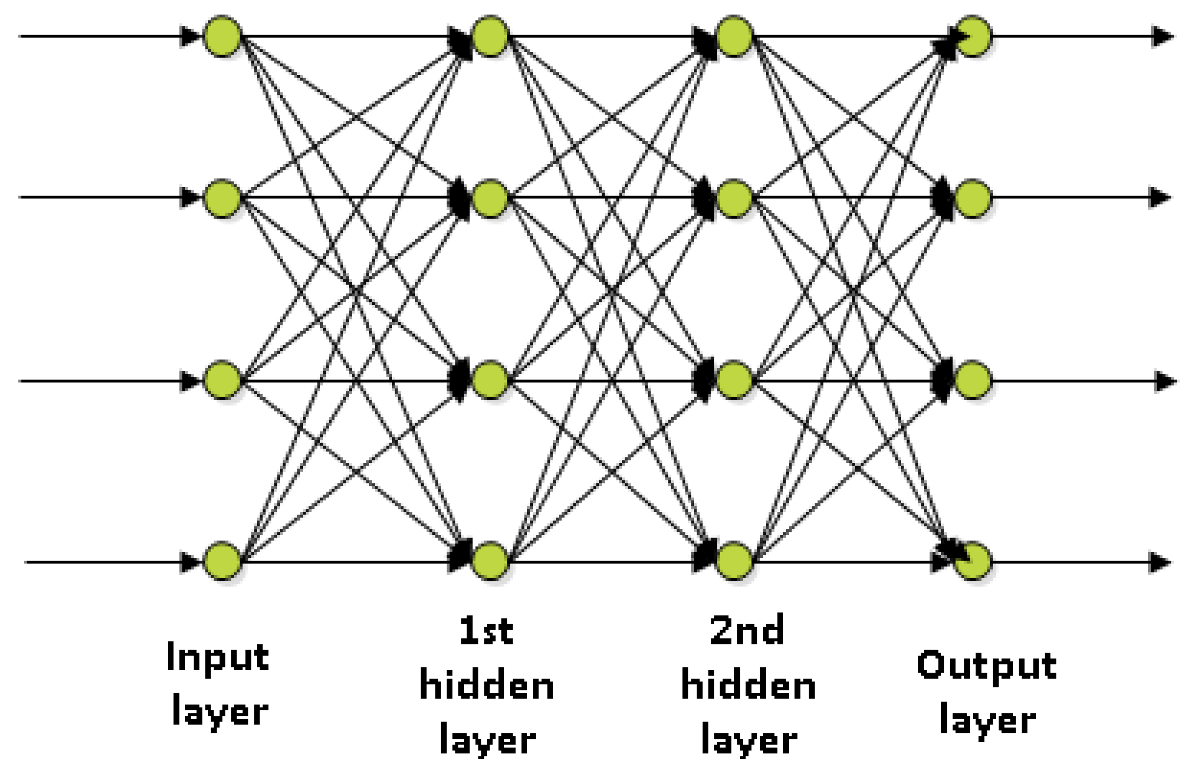
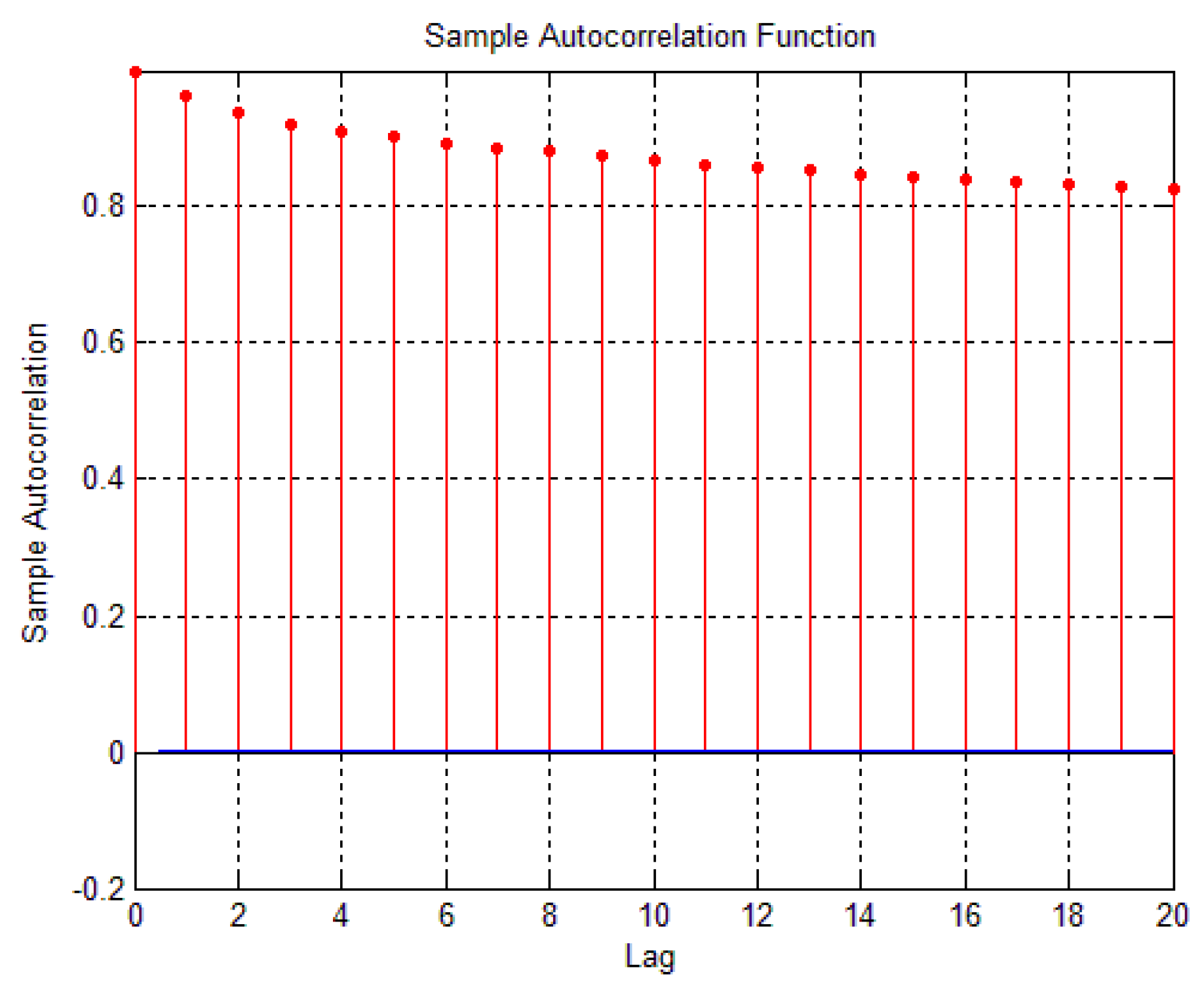
The forecasting models are distinguished into physical and statistical. Physical models take into consideration parameters like the topology of the ground (for on-site parks) and topology of the wind park and temperature. They use the outputs of a Numerical Weather Prediction (NWP) model and provide final forecasts. NWP models are used by meteorologists and usually they provide predictions for the next 48 up to 172 h ahead. For the case of wind power predictions, the wind speed prediction is obtained directly by the NWP and the wind power prediction is obtained by using the power curve of a wind turbine. Physical models are appropriate for long-term predictions. However, it is difficult to scale the forecasts per wind turbine or per wind farm. Also, physical models are complex in terms of inputs requirements and execution time. On the other hand, statistical models are favored in short-term prediction horizons. The wind is treated as a regression of its past values. A relatively large number of historical values are needed to train the models and define their optimal composition. Statistical models refer to time series models, Artificial Neural Networks, Bayesian Networks, Support Vector Machines, and others. Time series models refer to autoregressive models, autoregressive models with moving average, and others. The main advantages are their potential for removing the trend of time series and their availability in software packages. However, there is a difficulty in extracting the optimal structure of the model. Also, time series models require a large number of historical values and are not definitely suitable for highly nonlinear series. Neural networks are suitable for nonlinear series and are a favorable scheme in many forecasting problems. Support vector machines are also a well-known forecasting engine but they demand large durations for their training and their parameters are optimized by a relatively complex process. Bayesian networks are more appropriate for small data sets. Finally, various statistical models can be integrated to form ensemble forecasting models [4,5,6,7,8,9,10,11].
In (Sfetsos [12], 2002), a comparison takes place between a persistent model, autoregressive integrated moving average (ARIMA) and neural network. The latter outperforms the rest. No external variables are considered. The comparison takes place in two different sets that refer to one month each. In (Başaran and Filik [13], 2017) the authors consider three cases of inputs for the neural network, i.e., using only past wind speed values, using past wind speed values and temperature and, finally, using wind speed, temperature, and pressure. The test refers to five days and two intervals for predictions are taken into account, namely 30 and 90 s ahead. The case with wind speed, temperature, and pressure leads to the lower errors. No comparison with other models is presented. In (More and Deo [14], 2003) the authors test a feed-forward neural network, a recurrent neural network, and an ARIMA model to forecast daily, weekly, and monthly wind speeds at two coastal locations in India using only past wind speed values. The feed-forward neural network wins the competition. In (Li and Shi [15], 2010), the authors examine three types of neural networks, namely, the adaptive linear element, backpropagation, and radial basis function. The wind data used are the hourly mean wind speed collected at two observation sites in a United States of America (USA) location. The results show that even for the same wind dataset, no single neural network model outperforms others universally in terms of all evaluation metrics. Moreover, the selection of the type of neural networks for best performance is also depends upon the data sources. In (Zeng and Qiao [16], 2011) a support vector machine model is presented for wind power forecasting. Instead of predicting wind power directly, the model first predicts the wind speed, which is then used to predict the wind power by using the power–wind speed characteristics of the wind turbine generators. Simulation studies are carried out to validate the proposed model for very short-term and short-term predictions by using the data obtained from the National Renewable Energy Laboratory of USA. The model is compared with feed-forward neural network and radial basis network. The prediction is held using only past wind speed values. In (Zhou et al. [
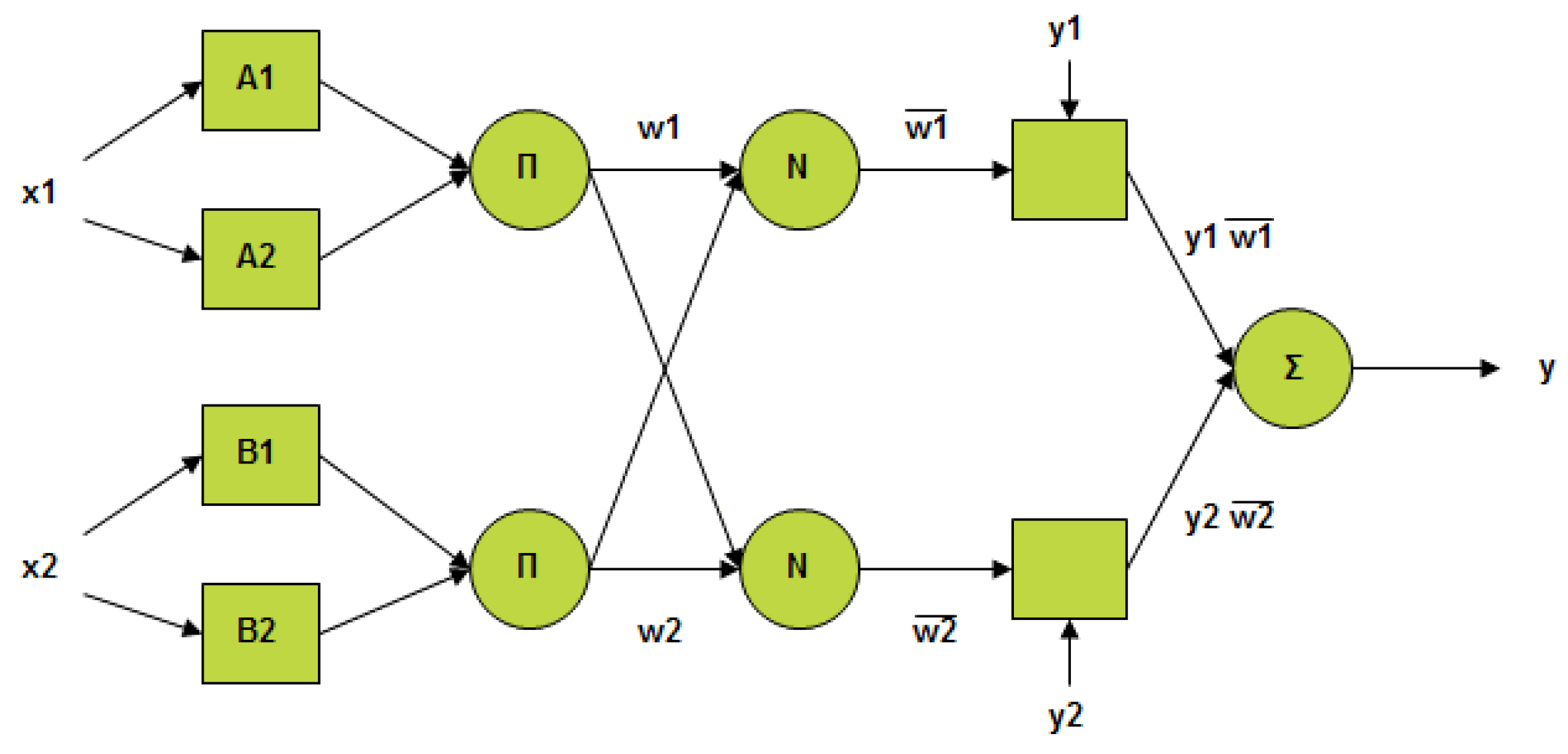
17], 2011), the authors present a least-squares support vector machine for one-step ahead wind speed forecasting. Three kernels, namely linear, Gaussian, and polynomial kernels, are implemented. The support vector machine‘s parameters considered include the training sample size, order, regularization parameter, and kernel parameters. The support vector machine‘s version are compared with a persistence model and provide better forecasts. The Adaptive Neuro-Fuzzy Inference System (ANFIS) is utilized in (Fazelpour et al. [18], 2016), and is compared with a feed-forward neural network and radial basis network in hour-ahead forecasting in a location in Tehran, Iran. No exogenous parameters are used. ANFIS results in better forecasts. In (Fortuna et al. [19], 2016), the clustering tool is used to form wind speed classes. Then, two models, namely the Hidden Markov Model and the Nonlinear Autoregressive are compared for predicting the class of each new wind speed data entry. In general, wind speed series present volatilities and stochasticity. Depending on the data set, an analysis on the wind speed characteristics can take place. For instance, in (Fortuna et al. [20], 2014), the authors provide a fractal analysis on wind speed observations. Exploitable information can be derived for such analysis for further modeling.

1.2. Contribution of the Present Paper

A variety of forecasting techniques have been proposed so far from different research groups. In the present paper a relatively simple yet efficient model for short-term wind speed forecasting based on real measured wind speed data is developed, applied, and proposed. The used data set involves inconsistencies of the time sequence of the wind speed series due to missing data. Various experiments take place that refer to different input combinations. Also, the Discrete Wavelet Transform (DWT) is utilized in order to decompose the initial series into a set of wavelet components for strengthening the forecasting credibility [21,22]. The model is composed by an ANFIS and a Feed-Forward Neural Network (FFNN) [23,24]. In the majority of the studies of the literature, the prediction is accomplished using only past values. In order to fully examine the level of influence of external variables such as temperature and speed directions on the prediction accuracy, in the present paper various input combinations of wind speed, wind direction, and air temperature are examined. Overall, the purpose of the paper is to test the performance of a proposed hybrid computational intelligence model in the wind speed forecasting problem under the limitation of using incomplete data for the training and validation of the model.

2. Short-Term Wind Speed Forecasting Hybrid Model

2.1. Description

In this section, an efficient forecasting model is developed and proposed. The model consists of an FFNN trained by the Levenberg–Marquardt algorithm and an ANFIS [25]. Neural network-based forecasting systems are a favorable scheme in recent years in predictions over traditional time series models. Numerous applications in load and price forecasting studies have brought forth the advantages of neural networks. Recently, neural networks have been used in wind power predictions. For full mathematical description of the FFNN the reader is referred to (Graupe [24], 2007). A general illustration of an FFNN is shown in Figure 1.
Another common forecasting system is ANFIS [23]. ANFIS is based on a fuzzy rule-based inference mechanism. It is composed of five layers and each layer contains several nodes. The nodes are described by a node function. Let O i j be the output of the i-th node in layer j. In the 1st layer, every node I is an adaptive node with node function:
O i 1 = μ A i ( x ) , i = 1 , 2
or
O i 1 = μ B i 2 ( y ) , i = 3 , 4
where x or y is the input of the ith node and A i or B i 2 is a linguistic label associated with the node. Hence, O i j is the membership grade of a fuzzy set A 1 , A 2 , B 1 or B 2 and it specifies the degree to which the input x or y satisfies the quantifier A or B. Any continuous and piecewise differential function can be used as node function in the 1st layer. In the 2nd layer, each node Π multiplies the inputs and sends the product in output:
O i 2 = w i = μ A i ( x ) μ B i ( y ) , i = 1 , 2
In the 3rd layer, each node N computes the ratio
O i 3 = w ¯ i = w i w 1 + w 2 , i = 1 , 2
In the 4th layer, each node computes the contribution of the ith rule to the overall output:
O i 4 = w ¯ i z i = w ¯ i ( a i x + b i y + c ) , i = 1 , 2
where w ¯ i is the output of the 3rd layer and a i , b i , c are a set of parameters.
Finally, in the 5th layer, the node Σ computes the final output as the summation of all inputs:
O i 5 = i w ¯ i z i = i w i z i i w i
ANFIS topology is displayed in Figure 2.
The proposed forecasting model combines the independent forecasts of FFNN and ANFIS. A schematic representation of the hybrid model is shown in Figure 3. The models are trained separately. The training set is used to define the optimal model parameters. For instance, for the case of the FFNN the parameters that need to be defined are the number of hidden layers, the number of neurons in the hidden layer, and the type of activation function in the hidden and output layers. While for the case of ANFIS the required parameters that need to be defined are the type of inference mechanism, the training epochs, the number of fuzzy rules, the type of membership function, and the values of a i , b i , c . Real monitored environmental data measured with a monitoring system are used in the present paper for developing the forecasting model. The monitoring system is placed in the coastal area of Neos Marmaras, Greece. Details about the monitoring system (e.g., sensors used and verification) can be found in (Michailides et al. [26], 2013). The training and test sets cover the periods 01/04/2013–10/08/2013 and 01/09/2013–24/12/2013, respectively. The test set is used for the comparison of the models. No filling of incomplete or missing data took place. Also, no other preprocessing of the data took place. The aim is to build a model applied to raw data obtained from a real measurement system.
The proposed model is applied to two different predictions test examples, i.e., 1 min-ahead and 10 min ahead. Five cases with different types of inputs are examined, namely Case#1, Case#2, Case#3, Case#4, and Case#5. The inputs considered in each case are described in the following.
-
Case#1: wind speed
-
Case#2: wind speed and wind direction
-
Case#3: wind speed and temperature
-
Case#4: wind speed, wind direction and temperature
-
Case#5: wavelet components of wind speed.
The topology of the proposed model using the wavelet components is shown in Figure 4.
Therefore, we examined ten different cases referring to the two prediction horizons.

2.2. Performance Assessment

The performance assessment includes a set of mathematical criteria that measure the prediction errors. To fully examine the proposed model performance, we used a set of different mathematical criteria. Let p m a and p m f be the actual and predicted wind speed values of the m-th day of the test set, m = 1, 2, …, M, respectively. The indicator considered for the assessment are the Absolute Error (AE), the Mean Absolute Error (MAE), the Root Mean Squared Error (RMSE), and the Mean Absolute Range Normalized Error (MARNE) as defined in Equation (10). The AE is defined as
AE = m = 1 M | p m a p m f |
The MAE corresponds to the sum of all AEs:
MAE = 1 M m = 1 M | p m a p m f |
The RMSE is expressed as
RMSE = 1 M m = 1 M ( p m a p m f ) 2
The MARNE is the absolute difference between the actual and forecast wind speed, normalized to the maximum wind speed:
MARNE = 1 M m = 1 M | p m a p m f | max ( p m a ) × 100
As benchmarks for the proposed model test, the individual applications of FFNN and ANFIS are used.

3. Simulation Results

3.1. Wind Speed Forecasting

Computational intelligence-based systems are a favourable scheme in recent years in various variable predictions, such as electric load, over traditional time series models. However, a careful selection of inputs and a proper training phase are essential for the model’s successful implementation and utilization. The selection of the types of inputs is crucial to the forecasting success. In the present study, various input combinations are examined. The objective is to test computational intelligence-based models for the case of incomplete data. Three models are compared that refer to an FFNN, an ANFIS, and a proposed FFNN-ANFIS. After the decision of the types of inputs, i.e., Case#1–Case#5, the next test is to define the number of inputs. This number refers to the historical values of the used parameters: wind speed, temperature and wind direction. With the application of the Sample Autocorrelation Function (SAF), the historical values are evaluated based on the correlation of the present value. Figure 5 displays the SAF that resembles the minute-ahead wind speed set. Only the first 20 values are displayed. It is shown that the correlation is decreasing progressively when the lagged value becomes more time distant. The same conclusions are drawn from the 10 min ahead set. The first five values are selected as inputs for the models. Also, the corresponding values of temperature and wind direction are proportionally selected.
Employing the minute-ahead set and the data set of Case#1, a series of experiments were conducted for the purpose of defining the optimal FFNN and ANFIS structures. The optimal FFNN structure has one hidden layer. The tangent sigmoid function is used both for the hidden and output layers. The number of training epochs is set equal to 100. The optimal number of neurons in the hidden layer is defined also by series of simulations. It differs among the various cases. Thus, a series of FFNN executions took place to track the number of hidden layers that minimize the RMSE indicator. Concerning the optimal ANFIS topology, the Sugeno inference method is selected together with Gaussian membership functions.
The scores of the forecasting models on the assessment indicators are presented at Table 1 and Table 2. Table 1 refers to the 1-min-ahead horizon and Table 2 to the 10-min-ahead horizon. The rows of the Tables correspond to the different cases. According to the results of Table 1, the proposed model outperforms the FFNN and ANFIS in all test cases, highlighting the significance of using combined forecasts. The prediction accuracy improvement that is obtained with the proposed model is more evident in the data sets of Case#3, Case#4, and Case#5. FFNN leads to better results compared to ANFIS in Case#2, Case#3, and Case#5 when using the MAE indicator. Also, the FFNN leads to better results in Case#1 according to the RMSE and MARNE measures. However, it scores in MARNE = 4.2353% in Case#2, a value that is higher than the respective of ANFIS. While in most experiments the FFNN appears more robust, it can be suggested over the ANFIS in the minute-ahead wind speed prediction problem.
Among the types of data inputs, Case#5 leads to considerably lower errors indicating the benefit of transforming the volatile wind data into the wavelet domain. This is evident in all measures and especially in MARNE. Considering the MAE indicator, Case#2 leads to better predictions if the latter is held with FFNN or the hybrid model. On the contrary, the data of Case#1, i.e., using only wind speed values is more suitable for ANFIS. Using wind speed, temperature, and wind direction as inputs, the prediction is less credible. This implies again for FFNN and the proposed model. ANFIS scores MAE = 0.4443 with the data of Case#3. The aforementioned conclusions are identical when the evaluation is held with the RMSE or MARNE. Therefore, by combining wind speed and direction data the forecasting procedure is strengthened. The use of temperature is not recommended for the test set under study. According to the above analysis, the combination of the FFNN and ANFIS that is fed with the wind speed data transformed in the wavelet domain is the recommended model for minute-ahead forecasts under the limitation of many incomplete data entries.
According to the findings presented in Table 2, it is evident that the 10-min-ahead wind speed prediction problem is a more difficult task. A possible reason for this is the decrease that is accomplished between current and past values of the minute time frame measurements. This means that the 10-min data are less correlated since the minute correlation lowers due to the averaging of the one-minute data for the purpose of transforming them in the 10-min intervals. The proposed FFNN-ANFIS model is more accurate than the rest in all types of data sets. Again the 10-min-ahead problem benefits from the implementation of the wavelet transform. The data of Case#5 provide more robust predictions independently of the model used.
A further comparison of the models is held via the AE distribution over time. The MAE indicator receives one value for a specific prediction, for example for a given number of neurons in the hidden layer. It is essential to examine the error distribution over the focusing period. Using the AE indicator, the analysis can be scaled to minutes. This concept strengthens the conclusions drawn from the models comparison. Figure 6 presents the AE distribution per Case. The figure refers to the 1-min-ahead prediction horizon while the forecasting is achieved with the proposed FFNN-ANFIS model. The discrete peaks correspond to large error values, which can be considered as indicators of the model’s poor performance for the specific minute. The data of Case#1–Case#4 lead to some high peaks of the AE shape. These are mainly met in December days. The lowest errors are mostly gathered in September days. As the time horizon progresses, the peaks become more frequent. Hence, extreme weather conditions worse the credibility of the predictions. Some late autumn and winter wind speeds are difficult to effectively be predicted in the coastal site under study. The mean values of AE are 0.3673, 0.3664, 0.4123, 0.4210, and 0.1021 for Case#1, Case#2, Case#3, Case#4, and Case#5, respectively. Some parallel conclusions with the above results can be made for the 10-min-ahead horizon. The corresponding results are graphically presented in Figure 7. In the 10-min-ahead problem, the implementation of the wavelet transform is more advantageous compared to the minute-ahead case. Case#5 increases the accuracy by a large portion. The mean values of AE are 0.4288, 0.4293, 0.4706, 0.4654, and 0.1227 for Case#1, Case#2, Case#3, Case#4, and Case#5, respectively.
In order to examine the relationship between the accuracy and the direction of the wind, we measured the AE per direction degree. Figure 8 shows the comparison among Case#2 and Case#5 for the 1-min-ahead forecasts. Case#2 refers to the combination of wind speed and direction. The predictions refer to the proposed model. Case#5 involves only to the transformed wind speed data. It is plotted here for the sake of comparison. The lowest AE of Case#2 is 5.97 × 10⁻⁶ and occurred for 312.48°. The next lowest AE degrees are 200.73°, 104.56°, 151.90°, and 281.14°. The larger values of AE are presented for 162.47°, 42.17°, 55.08°, and 222.70°. According to these findings, a preliminary conclusion is that there is no strong correlation between the direction and the forecasting error. For example, it can be strongly supported that normal to the monitoring system winds (e.g., 90°) are less predictable compared to other directions. This statement is also supported from the data of Case#5. The lowest errors refer to 134.67°, 122.06°, 73.07°, 317.51°, and 46.48° directions, while, the highest ones are occurred for 27.01°, 35.56°, 41.31°, 57.65°, and 31.57°. In this data set, the less accurate prediction is presented for wind direction degrees below 60°.
As illustrative examples of the proposed model’s behavior, Figure 9 and Figure 10 present the actual and forecasted wind speed curve of the test set for 1-min- and 10-min-ahead horizons, respectively. The forecasted wind speed sequences of the two figures succeed by a large portion to accurately simulate the actual data, which is another one indicator of the robustness of the model.

3.2. Comparison with Other Forecasting Models

To fully evaluate the proposed model, a comparison is made with the following models; Group Method of Data Handling Neural Network (GMDHNN) [27], Regression Neural Network (GRNN) [28], Regression Trees (RTs) [29], Relevance Vector Machine (RVM) [30], and Support Vector Regression (SVR) [31]. Table 3 and Table 4 present the scores of GMDHNN, GRNN and RTs, RVM and SVR, respectively, on the error metrics, for the 1-min-ahead predictions. Correspondingly, Table 5 and Table 6 present the scores of GMDHNN, GRNN and RTs, RVM and SVR, respectively, on the error metrics MAE, RMSE, and MARNE for 10-min-ahead predictions. Among these models, SVR and GMDHNN display comparative results with the hybrid model. The latter outperforms all the other models. It can be noticed that GRNN and RTs result in high errors and thus, for the problem under study are not recommended.

4. Discussion and Concluding Remarks

Offshore wind turbine installations are continually gathering the research interest since they are considered an efficient mechanism for covering the electrical needs of various isolated loads. The present study emphasizes on the development of an effective method for very short-term wind speed forecasting under the limitation of wind speed series that do not present consistency in time, i.e., there are interruptions in the date sequence. Real measured data are used for the training of the developed method. An ensemble data-driven short-term wind speed forecasting model is developed, tested, and applied. The term “ensemble” refers to the combination of two different predictors that run in parallel and the prediction is obtained by the predictor that leads to the lowest error. The proposed model utilizes the wavelet transform and is compared with other models that have been presented in the related literature. The main conclusions of the present study:
  • The proposed forecasting model can be used effectively for 1 min and 10 min ahead horizon wind speed predictions.
  • The exogenous variables (i.e., wind speed direction and air temperature) decrease the prediction accuracy. The best results are obtained using the DWT.
  • The highest errors are met on winter days and especially in instances with high wind speed.
  • There is no correlation among the forecasting error and the wind direction.
  • The hybrid model (combination of FFNN and ANFIS) leads to better forecasts in all examined data set cases.
  • The proposed model outperforms the accuracy of other forecasting models that have been presented in the related literature.
The research of the present paper will be further expanding by checking the implementation of the forecasting problem in the Wind Farm Layout Optimization (WLFO) problem incorporating wake effects with the use of specific mathematical or numerical models. Forecasted wind speed time series can serve as inputs to the problem. By estimating future wind speed values, the WLFO can be modified to a scenario-based problem where different wind speed forecasts can lead to various WLFO solutions and thus, assessing the level of influence of the future wind speed variations in the outputs of the optimization problem.

Author Contributions

I.P.P. performed the research and wrote the first draft of the paper. C.M. and D.C.A. set the objectives of the research, provided guidance for the research, and revised the paper.

Funding

This research received no external funding.

Conflicts of Interest

The authors declare no conflicts of interest.

References

  1. WindEurope. Offshore Wind in Europe Key Trends and Statistics 2018. Available online: https://windeurope.org/wp-content/uploads/files/about-wind/statistics/WindEurope-Annual-Offshore-Statistics-2018.pdf (accessed on 27 March 2019).
  2. Snyder, B.; Kaiser, M.J. A comparison of offshore wind power development in Europe and the US: Patterns and drivers of development. Appl. Energy 2009, 86, 1845–1856. [Google Scholar] [CrossRef]
  3. Soman, S.S.; Zareipour, H.; Malik, O.; Mandal, P. A review of wind power and wind speed forecasting methods with different time horizons. In Proceedings of the 2010 North American Power Symposium, Arlington, TX, USA, 26–28 September 2010; pp. 1–8. [Google Scholar]
  4. Jung, J.; Broadwater, R.P. Current status and future advances for wind speed and power forecasting. Renew. Sustain. Energy Rev. 2014, 31, 762–777. [Google Scholar] [CrossRef]
  5. Okumus, I.; Dinler, A. Current status of wind energy forecasting and a hybrid method for hourly predictions. Energy Conves. Manag. 2016, 123, 362–371. [Google Scholar] [CrossRef]
  6. Lei, M.; Shiyan, L.; Chuanwen, J.; Hongling, L.; Ya, Z. A review on the forecasting of wind speed and generated power. Renew. Sustain. Energy Rev. 2009, 13, 915–920. [Google Scholar] [CrossRef]
  7. Chang, W.Y. A literature review of wind forecasting methods. J. Power Energy Eng. 2014, 2, 161–168. [Google Scholar] [CrossRef]
  8. Foley, A.M.; Leahy, P.G.; Marvuglia, A.; McKeogh, E.J. Current methods and advances in forecasting of wind power generation. Renew. Energy 2012, 37, 1–8. [Google Scholar] [CrossRef]
  9. Bhaskar, M.; Jain, A.; Srinath, N.V. Wind speed forecasting: Present status. In Proceedings of the 2010 International Conference on Power System Technology, Hangzhou, China, 24–28 October 2010; pp. 1–7. [Google Scholar]
  10. Murthal, D. Wind power forecasting: A survey. Int. J. Eng. Res. Gen. Sci. 2016, 4, 802–806. [Google Scholar]
  11. Tascikaraoglu, A.; Uzunoglu, M. A review of combined approaches for prediction of short-term wind speed and power. Renew. Sustain. Energy Rev. 2014, 34, 234–254. [Google Scholar] [CrossRef]
  12. Sfetsos, A. A novel approach for the forecasting of mean hourly wind speed time series. Renew. Energy 2002, 27, 163–174. [Google Scholar] [CrossRef]
  13. Başaran, Ü.; Filik, T. Wind speed prediction using artificial neural networks based on multiple local measurements in Eskisehir. Energy Procedia 2017, 107, 264–269. [Google Scholar]
  14. More, A.; Deo, M.C. Forecasting Wind with Neural Networks. Mar. Struct. 2003, 16, 35–49. [Google Scholar] [CrossRef]
  15. Li, G.; Shi, J. On comparing three artificial neural networks for wind speed forecasting. Appl. Energy 2010, 87, 2313–2320. [Google Scholar] [CrossRef]
  16. Zeng, J.W.; Qiao, W. Support vector machine-based short-term wind power forecasting. In Proceedings of the 2011 IEEE/PES Power Systems Conference and Exposition, Phoenix, AZ, USA, 20–23 March 2011; pp. 1–8. [Google Scholar]
  17. Zhou, J.Y.; Shi, J.; Li, G. Fine tuning support vector machines for short-term wind speed forecasting. Energy Convers. Manag. 2011, 52, 1990–1998. [Google Scholar] [CrossRef]
  18. Fazelpour, F.; Tarashkar, N.; Rosen, M.A. Short-term wind speed forecasting using artificial neural networks for Tehran. Iran. Int. J. Energy Environ. Eng. 2016, 7, 377–390. [Google Scholar] [CrossRef]
  19. Fortuna, L.; Guariso, G.; Nunnari, S. One day ahead prediction of wind speed class by statistical models. Int. J. Renew. Energy Res. 2016, 6, 1137–1145. [Google Scholar]
  20. Fortuna, L.; Nunnari, S.; Guariso, G. Fractal order evidences in wind speed time series. In Proceedings of the 2014 International Conference on Fractional Differentiation and Its Applications, Catania, Italy, 23–25 June 2014; pp. 1–6. [Google Scholar]
  21. Mallat, S. A theory for multiresolution signal decomposition-the wavelet representation. IEEE Trans. Pattern Anal. Mach. Intell. 1989, 11, 674–693. [Google Scholar] [CrossRef]
  22. Amjady, N.; Keynia, F. Short-term load forecasting of power systems by combination of wavelet transform and neuro-evolutionary algorithm. Energy 2009, 34, 46–57. [Google Scholar] [CrossRef]
  23. Jang, J.S.R. ANFIS: Adaptive-network-based fuzzy inference system. IEEE Trans. Syst. Man Cybern. 1993, 23, 665–685. [Google Scholar] [CrossRef]
  24. Graupe, P. Principles of Artificial Neural Networks, 2nd ed.; World Scientific: Singapore, 2007. [Google Scholar]
  25. Levenberg, K. A method for the solution of certain non-linear problems in least squares. Q. J. Appl. Math. 1944, 2, 164–168. [Google Scholar] [CrossRef]
  26. Michailides, C.; Loukogeorgaki, E.; Angelides, D.C. Monitoring the response of connected moored floating modules. In Proceedings of the Twenty-third International Offshore and Polar Engineering, Anchorage, AK, USA, 30 June–5 July 2013; pp. 869–876, ISBN 978-1-880653-99–9. [Google Scholar]
  27. Abdel-Aal, R.E.; Elhadidy, M.A.; Shaahid, S.M. Modeling and forecasting the mean hourly wind speed time series using GMDH-based abductive networks. Renew. Energy 2009, 34, 1686–1699. [Google Scholar] [CrossRef]
  28. Kumar, G.; Malik, H. Generalized regression neural network based wind speed prediction model for western region of India. Procedia Comput. Sci. 2016, 93, 26–32. [Google Scholar] [CrossRef]
  29. Troncoso, A.; Salcedo-Sanz, S.; Casanova-Mateo, C.; Riquelme, J.C.; Prieto, L. Local models-based regression trees for very short-term wind speed prediction. Renew. Energy 2015, 81, 589–598. [Google Scholar] [CrossRef]
  30. Sun, G.; Chen, Y.; Wei, Z.; Li, X.; Cheung, K.W. Day-ahead wind speed forecasting using relevance vector machine. J. Appl. Math. 2014, 2014, 1–6. [Google Scholar] [CrossRef]
  31. Botha, N.; van der Walt, C.M. Forecasting wind speed using support vector regression and feature selection. In Proceedings of the 2017 Pattern Recognition Association of South Africa and Robotics and Mechatronics, Bloemfontein, South Africa, 29 November–1 December 2017; pp. 181–186. [Google Scholar]
Figure 1. A Feed-Forward Neural Network (FFNN) with 4 inputs, 4 outputs, and 2 hidden layers.
Electronics 08 00420 g001
Figure 2. A general illustration of Adaptive Neuro-Fuzzy Inference System (ANFIS).
Electronics 08 00420 g002
Figure 3. Structure of the proposed forecasting model.
Electronics 08 00420 g003
Figure 4. Structure of the proposed forecasting model using the wavelet components.
Electronics 08 00420 g004
Figure 5. Sample autocorrelation function values of the wind speed data set.
Electronics 08 00420 g005
Figure 6. Absolute error of the proposed model corresponding at (a) Case#1, (b) Case#2, (c) Case#3, (d) Case#4, and (e) Case#5 of the 1-min-ahead prediction horizon.
Electronics 08 00420 g006
Figure 7. Absolute Error per time frame of the proposed model corresponding at (a) Case#1, (b) Case#2, (c) Case#3, (d) Case#4, (e) Case#5 of the 10-min-ahead prediction horizon.
Electronics 08 00420 g007
Figure 8. Absolute error per wind direction of the proposed model corresponding at (a) Case#2 and (b) Case#5 of the 1-min-ahead prediction horizon.
Electronics 08 00420 g008
Figure 9. Forecasted and actual series of the test set referring to the 1-min-ahead prediction horizon for all the examined time period (a), between 0 and 10,000 s (b), between 20,000 and 30,000 s (c), and between 40,000 and 50,000 s (d).
Electronics 08 00420 g009aElectronics 08 00420 g009b
Figure 10. Forecasted and actual series of the test set referring to the 10 min ahead prediction horizon for all the examined time period (a), between 0 and 1000 s (b), between 2000 and 3000 s (c), and between 4000 and 5000 s (d).
Electronics 08 00420 g010
Table 1. Comparison of the forecasting models considering the minute-ahead horizon.
MAERMSEMARNE (%)
FFNNANFISFFNN-ANFISFFNNANFISFFNN-ANFISFFNNANFISFFNN-ANFIS
Case#10.36830.36750.36730.55760.55780.55632.33652.33112.3298
Case#20.36760.36820.36640.75100.55920.55512.59522.33562.3242
Case#30.41230.44430.38870.72370.91630.64352.61532.81852.4658
Case#40.44060.42100.40910.92060.80440.75112.79472.67032.5952
Case#50.10210.13240.08120.15280.20520.13010.64770.84030.5601
Table 2. Comparison of the forecasting models considering the 10-min-ahead horizon.
MAERMSEMARNE (%)
FFNNANFISFFNN-ANFISFFNNANFISFFNN-ANFISFFNNANFISFFNN-ANFIS
Case#10.43160.42960.42870.62580.62650.62404.22804.20884.2008
Case#20.43230.42950.42920.62530.62630.62394.23534.20774.2054
Case#30.47060.49850.46050.75690.93730.68514.61044.88414.5115
Case#40.46540.49360.45280.71550.87190.66894.55944.83634.4367
Case#50.12270.15720.11010.16930.22260.15561.0771.54090.9967
Table 3. Evaluation of Group Method of Data Handling (GMDH), Regression Neural Network (GRNN), and Regression Trees (RTs) considering the 1-min-ahead horizon.
MAERMSEMARNE (%)
GMDHNNGRNNRTsGMDHNNGRNNRTsGMDHNNGRNNRTs
Case#10.36880.38460.44320.56890.57210.63312.34112.38693.1256
Case#20.37010.39100.45090.70510.76440.81092.45782.47713.2672
Case#30.36980.42560.47810.71890.73670.79922.58712.62253.4155
Case#40.39440.42010.45410.89020.90121.10912.71122.99043.6203
Case#50.10940.13880.16920.14810.15560.20120.62890.65520.7154
Table 4. Evaluation of Relevance Vector Machine (RVM) and Support Vector Regression (SVR) considering the 1-min-ahead horizon.
MAERMSEMARNE (%)
RVMSVRRVMSVRRVMSVR
Case#10.37210.37040.56140.53772.34822.3345
Case#20.39330.38650.75970.70292.47542.3419
Case#30.38850.38930.74080.69112.61722.5678
Case#40.38210.37830.89280.87092.92322.6213
Case#50.12770.11780.15420.14210.65240.5772
Table 5. Evaluation of GMDH, GRNN, and RTs considering the 10-min-ahead horizon.
MAERMSEMARNE (%)
GMDHNNGRNNRTsGMDHNNGRNNRTsGMDHNNGRNNRTs
Case#10.42920.45250.58980.62580.65530.80934.20514.43265.7812
Case#20.43020.55970.59010.62720.67150.80954.21494.50315.7812
Case#30.47040.69270.61570.68620.73420.84614.63344.78626.0319
Case#40.46010.60560.61080.67150.69890.80124.51304.69025.7568
Case#50.12380.16240.17990.16010.18330.21091.26711.48841.6117
Table 6. Evaluation of RVM and SVR considering the 10-min-ahead horizon.
MAERMSEMARNE (%)
RVMSVRRVMSVRRVMSVR
Case#10.43420.42980.63590.62684.25414.2206
Case#20.43510.43070.64400.62684.26304.2198
Case#30.53700.46810.86490.75295.26054.5365
Case#40.49880.46440.78980.74595.11334.5301
Case#50.14240.13080.20370.16541.58931.1276

