Characterization and Correction of the Geometric Errors in Using Confocal Microscope for Extended Topography Measurement. Part I: Models, Algorithms Development and Validation


Abstract
:1. Introduction
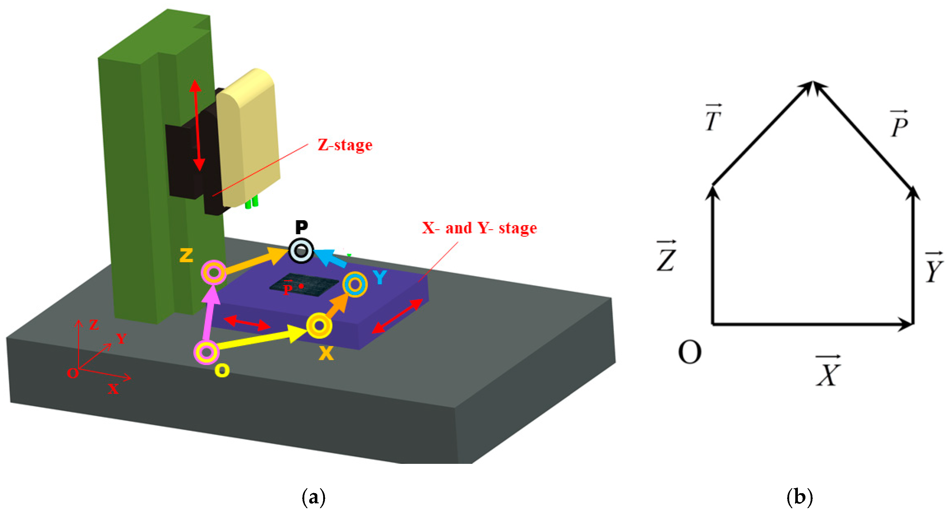
2. Mathematical Model for the X- and Y-Scale Calibration
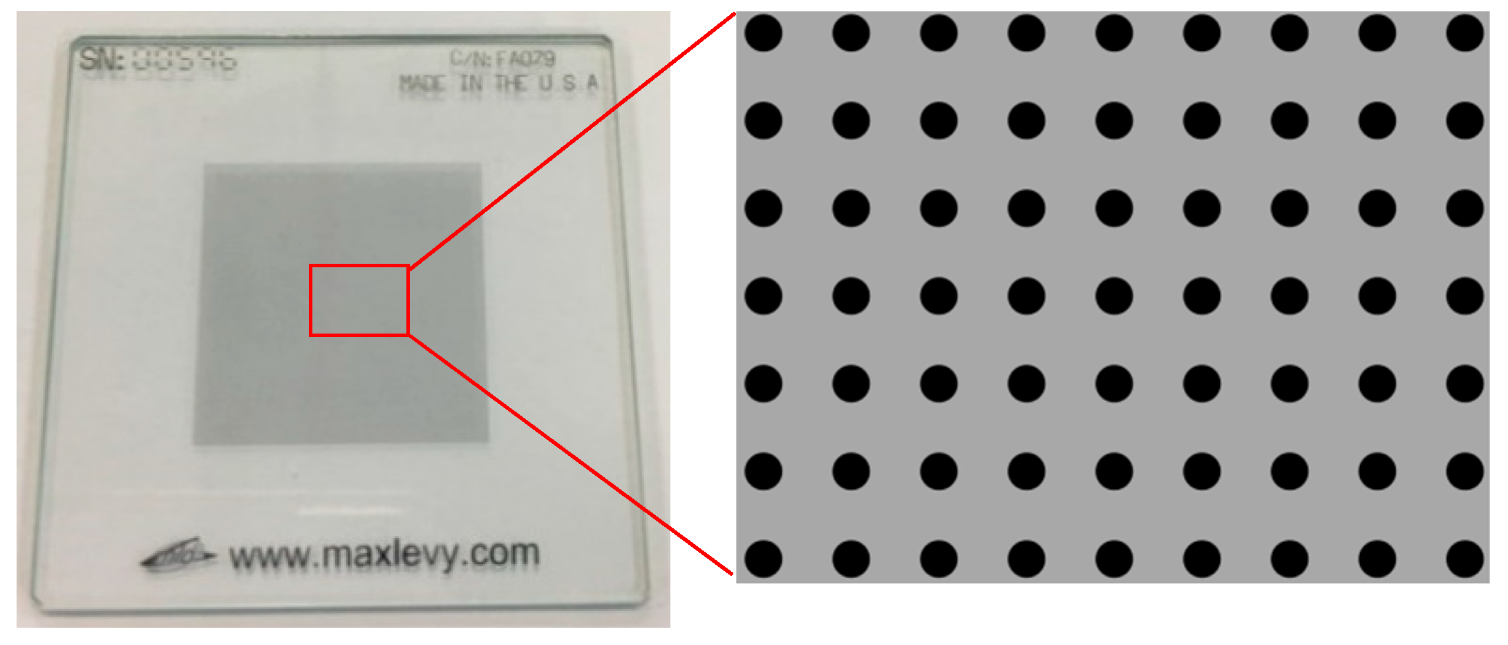
3. Methodology and a Brief Introduction of Experimental Design
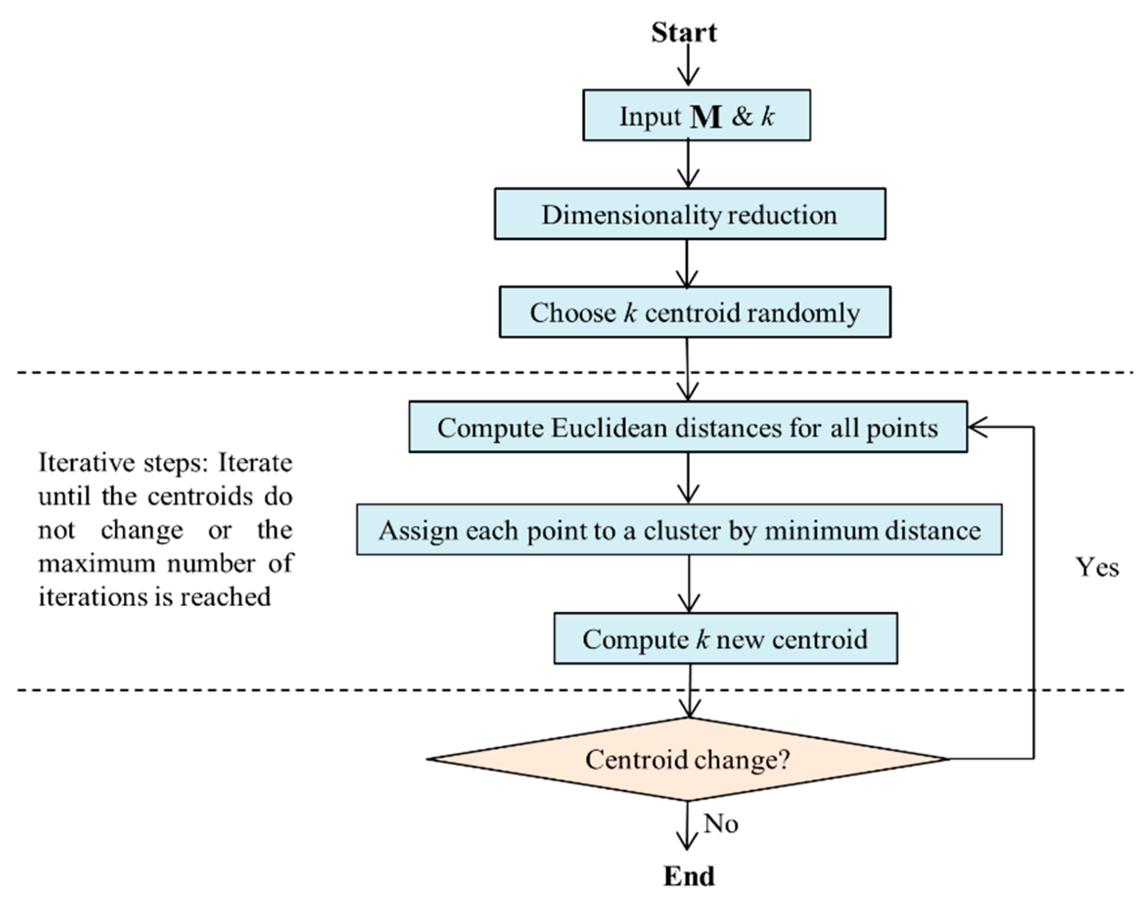
4. Algorithms and Procedures for Measurement Data Processing
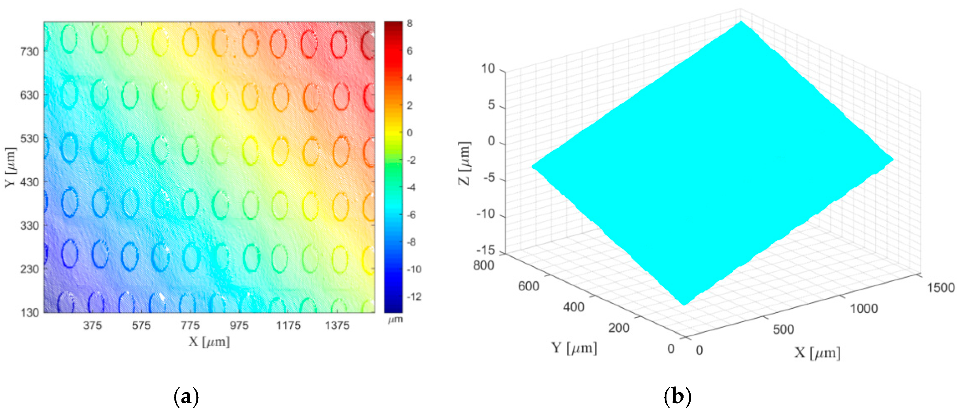
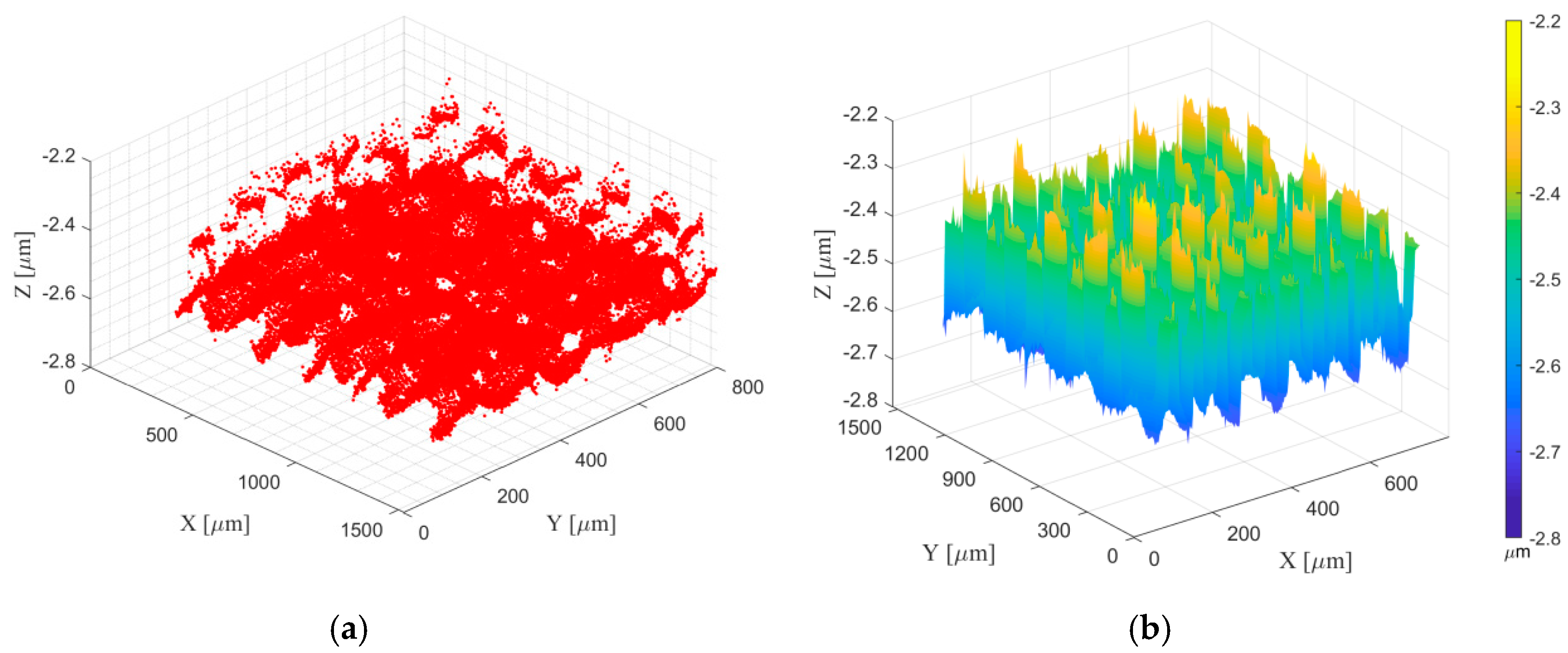
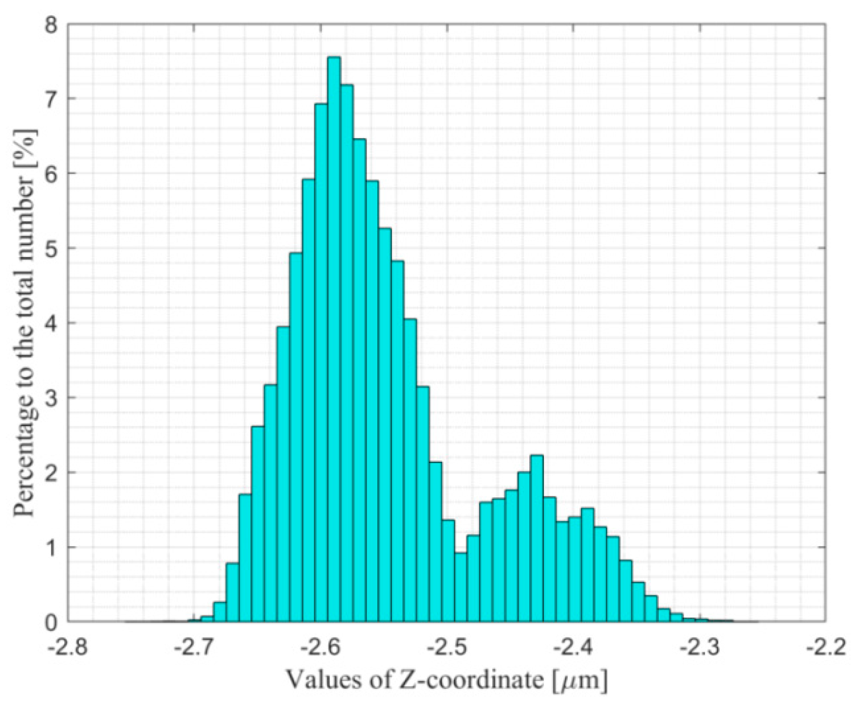
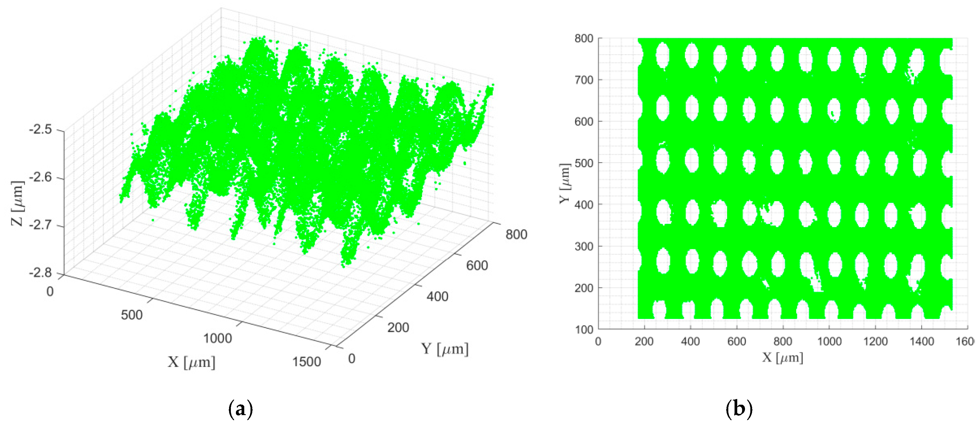
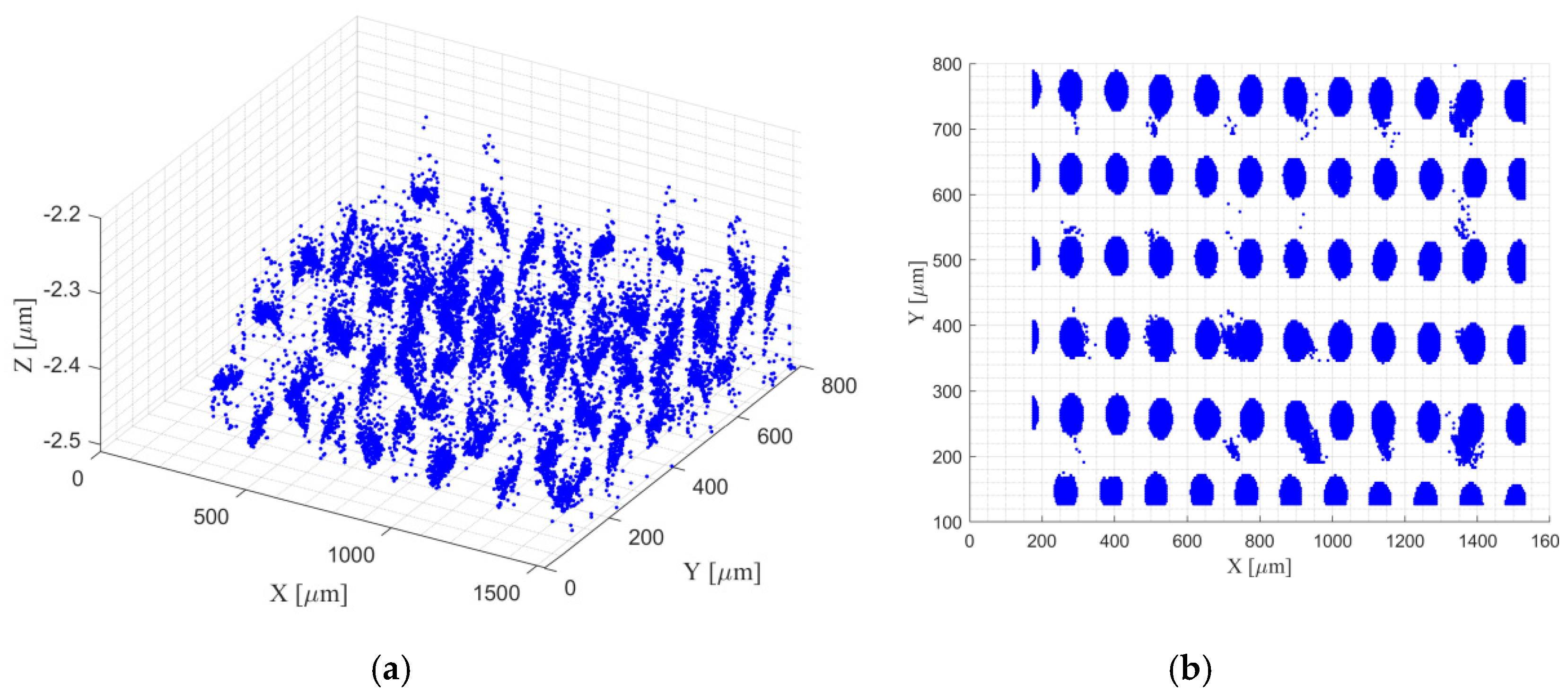
4.1. Algorithm and Procedure for the Separation of Flats and Cylinders
4.2. Algorithm for Determination of Coefficients
5. Validation of the Algorithms with Synthetic Data
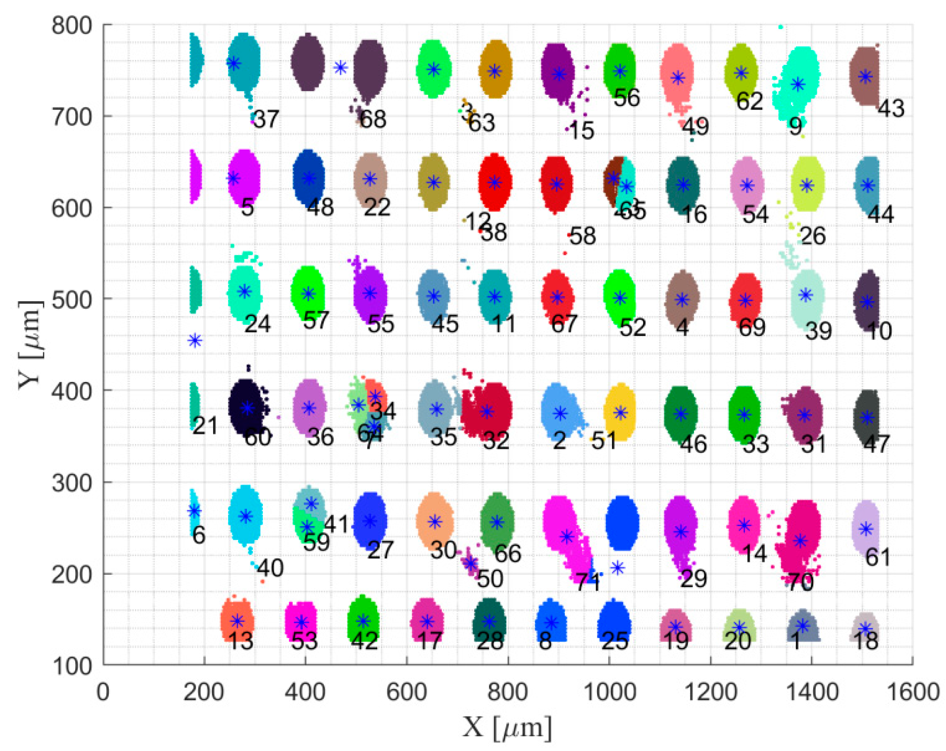
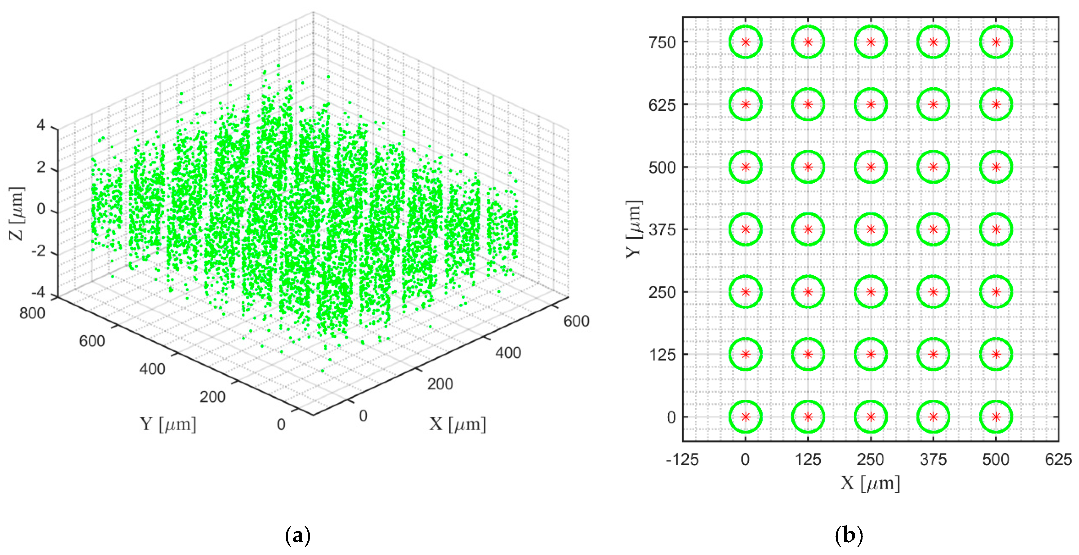
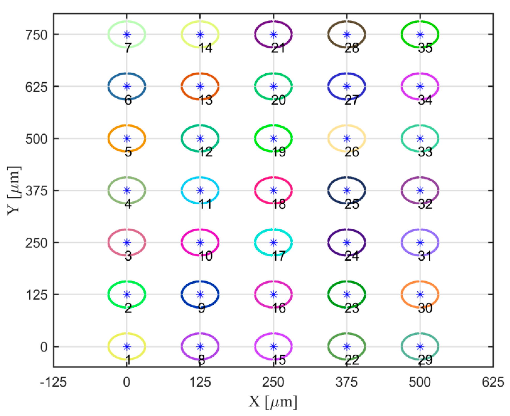
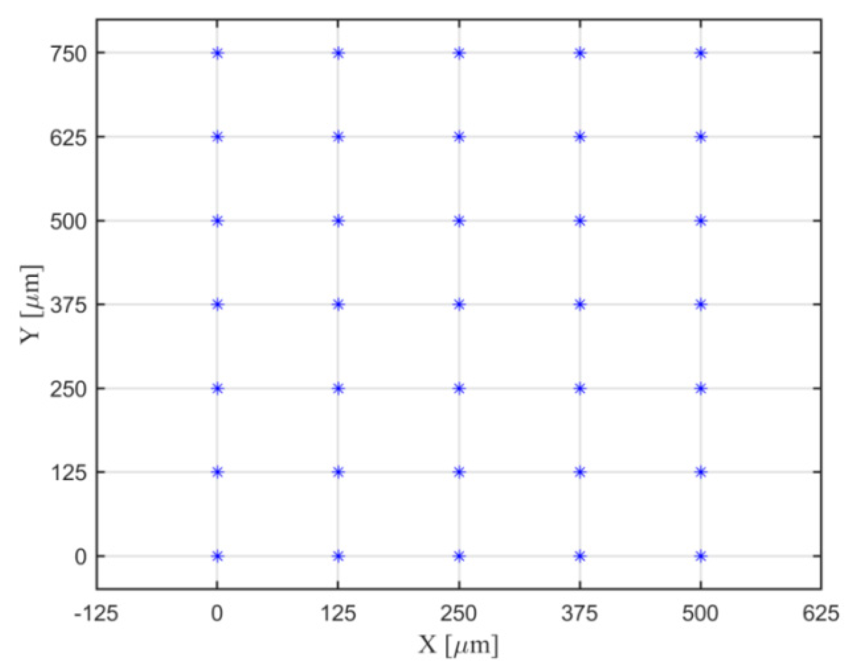
5.1. Validation of the Algorithm for Determination of Dots’ Centers and Distance
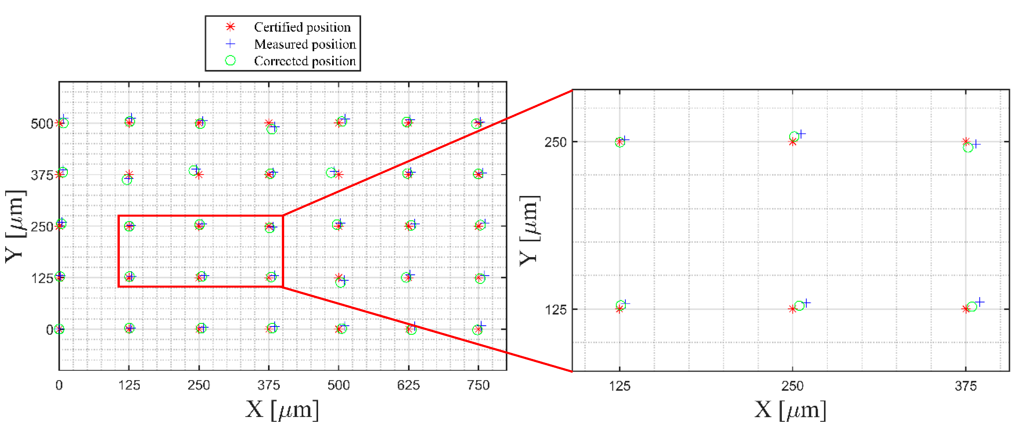
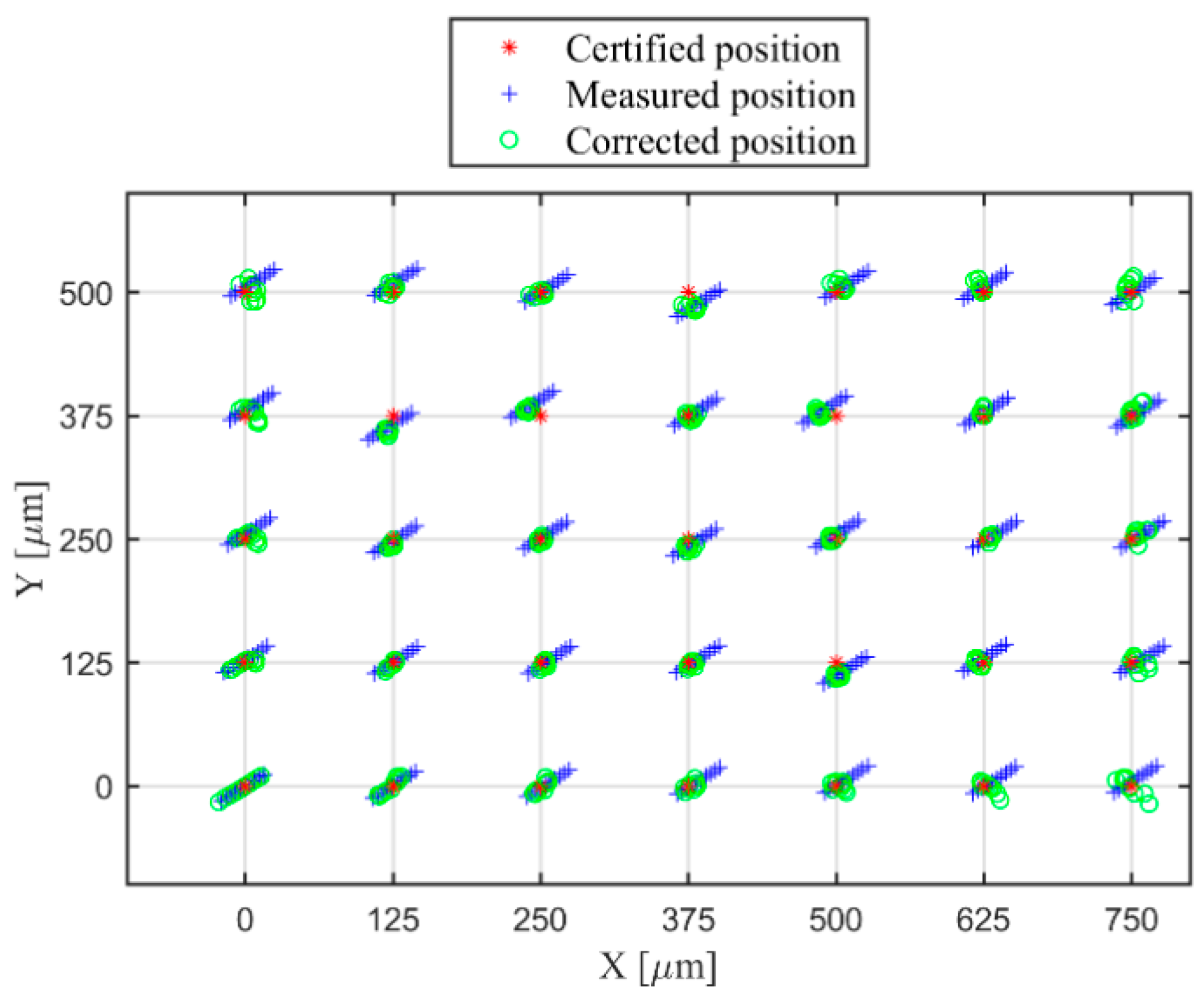
5.2. Validation of the Algorithm for Determination of Coefficients
6. Conclusions
Author Contributions
Funding
Conflicts of Interest
Abbreviations
| CM | confocal microscope |
| CCD | charge-coupled device |
| CMM | coordinate measuring machine |
References
- Zhang, G.; Ouyang, R.; Lu, B.; Hocken, R.; Veale, R.; Donmez, A. A Displacement Method for Machine Geometry Calibration. CIRP Ann. 1988, 37, 515–518. [Google Scholar] [CrossRef]
- Hermann, G. Geometric Error Correction in Coordinate Measurement. Acta Polytech. Hung. 2007, 4, 47–62. [Google Scholar]
- Krolczyk, G.M.; Maruda, R.W.; Nieslony, P.; Wieczorowski, M. Surface morphology analysis of Duplex Stainless Steel (DSS) in Clean Production using the Power Spectral Density. Measurement 2016, 94, 464–470. [Google Scholar] [CrossRef]
- Krolczyk, G.M.; Krolczyk, J.B.; Maruda, R.W.; Legutko, S.; Tomaszewski, M. Metrological changes in surface morphology of high-strength steels in manufacturing processes. Measurement 2016, 88, 176–185. [Google Scholar] [CrossRef]
- Wang, C.; D’Amato, R.; Gómez, E. Confidence Distance Matrix for outlier identification: A new method to improve the characterizations of surfaces measured by confocal microscopy. Measurement 2019, 137, 484–500. [Google Scholar] [CrossRef]
- Harding, K. (Ed.) Handbook of Optical Dimensional Metrology; CRC Press, Taylor & Francis Group: Boca Raton, FL, USA, 2013. [Google Scholar]
- Corle, T.R.; Kino, G.S. Confocal Scanning Optical Microscopy and Related Imaging Systems; Academic Press: Cambridge, MA, USA, 1996. [Google Scholar]
- Thomas, D.; Sugimoto, A. Parametric surface representation with bump image for dense 3d modeling using an rbg-d camera. Int. J. Comput. Vis. 2017, 123, 206–225. [Google Scholar] [CrossRef]
- Bailey, D.G. A new approach to lens distortion correction. Proc. Image Vis. Comput. N. Z. 2002, 2002, 59–64. [Google Scholar]
- Wang, J.; Shi, F.; Zhang, J.; Liu, Y. A new calibration model of camera lens distortion. Pattern Recognit. 2007, 41, 607–615. [Google Scholar] [CrossRef]
- Besseling, T.H.; Jose, J.; Van Blaaderen, A. Methods to calibrate and scale axial distances in confocal microscopy as as function of refractive index. J. Microsc. 2015, 257, 142–150. [Google Scholar] [CrossRef]
- Cole, R.W.; Jinadasa, T.; Brown, C.M. Measuring and interpreting point spread functions to determine confocal microscope resolution and ensure quality control. Nat. Protoc. 2011, 6, 1929–1941. [Google Scholar] [CrossRef]
- Wang, C. Current issues on 3D volumetric positioning accuracy: Measurement, Compensation and Definition. Proc. SPIE 2008, 7128. [Google Scholar] [CrossRef]
- Barakat, N.A.; Elbestawi, M.A.; Spence, A.D. Kinematic and geometric error compensation of a coordinate measuring machine. Int. J. Mach. Tools Manuf. 2000, 40, 833–850. [Google Scholar] [CrossRef]
- Zhang, G.; Veale, R.; Charlton, T.; Borchardt, B.; Hocken, R. Error Compensation of Coordinate Measuring Machines. CLRP Ann. 1985, 34, 445–448. [Google Scholar] [CrossRef]
- Schwenke, H.; Knapp, W.; Haitjema, H.; Weckenmann, A.; Schmitte, R.; Delbressine, F. Geometric error measurement and compensation of machines—An update. CIRP Ann. 2008, 57, 660–675. [Google Scholar] [CrossRef]
- Umetsu, K.; Furutnani, R.; Osawa, S.; Takatsuji, T.; Kurosawa, T. Geometric calibration of a coordinate measuring machine using a laser tracking system. Meas. Sci. Technol. 2005, 16, 2466–2472. [Google Scholar] [CrossRef]
- Semwogerere, D.; Weeks, E.R. Confocal Microscopy; Taylor & Francis: Abingdon, UK, 2005. [Google Scholar]
- Jensen, K.E.; Weitz, D.A.; Spaepen, F. Note: A three-dimensional calibration device for the confocal microscope. Rev. Sci. Instrum. 2013, 84, 016108. [Google Scholar] [CrossRef] [PubMed] [Green Version]
- Senin, N.; Leach, R. Information-rich surface metrology. Procedia CIRP 2018, 75, 19–26. [Google Scholar] [CrossRef]
- Claxton, N.S.; Fellers, T.J.; Davidson, M.W. Laser Scanning Confocal Microscopy; Technical Report; Department of Optical Microscopy and Digital Imaging, Florida State University: Tallahassee, FL, USA, 2006. [Google Scholar]
- ISO 25178-600. Geometrical Product Specifications (GPS)—Surface Texture: Areal-Part 600: Metrological Characteristics for Areal-Topography Measuring Methods; International Organization for Standardization: Geneva, Switzerland, 2019. [Google Scholar]
- Leach, R.K.; Giusca, C.L.; Haitjema, H.; Evans, C.; Jiang, X. Calibration and verification of areal surface texture measuring instruments. CIRP Ann. 2015, 64, 797–813. [Google Scholar] [CrossRef]
- Alburayt, A.; Syam, W.P.; Leach, R. Lateral scale calibration for focus variation microscopy. Meas. Sci. Technol. 2018, 29, 065012. [Google Scholar] [CrossRef]
- Leach, R. Optical Measurement of Surface Topography; Springer: Berlin, Germany, 2011. [Google Scholar]
- Nouira, H.; El-Hayek, N.; Yuan, X.; Anwer, N.; Salgado, J. Metrological characterization of optical confocal sensors measurements (20 and 350 travel ranges). J. Phys. Conf. Ser. 2015, 483, 012015. [Google Scholar] [CrossRef]
- Tong, K.; Lehtihet, E.A.; Joshi, S. Parametric error modeling and software error compensation for rapid prototyping. Rapid Prototyp. J. 2003, 9, 301–313. [Google Scholar] [CrossRef]
- Ekinci, T.O.; Mayer, J.R.R.; Cloutier, G.M. Investigation of accuracy of aerostatic guideways. Int. J. Mach. Tools Manuf. 2009, 49, 478–487. [Google Scholar] [CrossRef]
- Ekinci, T.O.; Mayer, J.R.R. Relationships between straightness and angular kinematic errors in machines. Int. J. Mach. Tools Manuf. 2007, 47, 1997–2004. [Google Scholar] [CrossRef]
- Yang, J.; Ren, Y.; Wang, C.; Liotto, G. Theoretical derivations of 4 body diagonal displacement errors in 4 machine configurations. In Proceedings of the LAMDAMAP Conference, Cransfield, UK, 27–30 June 2005. [Google Scholar]
- Aguado, S.; Samper, D.; Santolaria, J.; Aguilar, J.J. Towards an effective identification strategy in volumetric error compensation of machine tools. Meas. Sci. Technol. 2012, 23, 065003. [Google Scholar] [CrossRef]
- Wang, C.; Caja, J.; Gomez, E. Comparison of methods for outlier identification in surface characterization. Measurement 2018, 117, 312–325. [Google Scholar] [CrossRef]
- Hartigan, J.A.; Wong, M.A. A K-means Clustering Algorithm. J. R. Stat. Soc. 1979, 28, 100–108. [Google Scholar]
- Jain, K. Data clustering: 50 years beyond K-means. Pattern Recognit. Lett. 2010, 31, 651–666. [Google Scholar] [CrossRef]
- Lloyd, S.P. Least Squares Quantization in PCM. IEEE Trans. Inf. Theory 1982, 28, 129–137. [Google Scholar] [CrossRef]
- Ghodsi, A. Dimensionality Reduction—A Short Tutorial; Technical Report; University of Waterloo: Waterloo, ON, Canada, 2006. [Google Scholar]
- Sorzano, S.; Vargas, J.; Montano, A.P. A survey of dimensionality reduction techniques, Technical Report. arXiv 2014, arXiv:1403.2877. [Google Scholar]
- Miller, S.J. The Method of Least Squares; Brown University: Providence, RI, USA, 2006. [Google Scholar]
- Weisstein, E.W. Least Squares Fitting, From MathWorld–A Wolfram Web Resource. Available online: http://mathworld.wolfram.com/LeastSquaresFitting.html (accessed on 1 October 2018).
- Dennis, J.E.; Gay, D.M.; Welsch, R.E. An adaptive nonlinear least-squares algorithm. ACM Trans. Math. Softw. 1981, 7, 348–368. [Google Scholar] [CrossRef]
- Marquardt, D.W. An algorithm for Least-Squares estimation of nonlinear parameters. J. Soc. Ind. Appl. Math. 1963, 11, 431–441. [Google Scholar] [CrossRef]


| Width [mm] | Dot Diameter [mm] | Dot Spacing [mm] | X and Y Axis Accuracy [mm] | Dot Array | ||
|---|---|---|---|---|---|---|
| X | Y | Total | ||||
| 25 | 0.0625 | 0.125 | ±0.001 | 201 | 201 | 40401 |
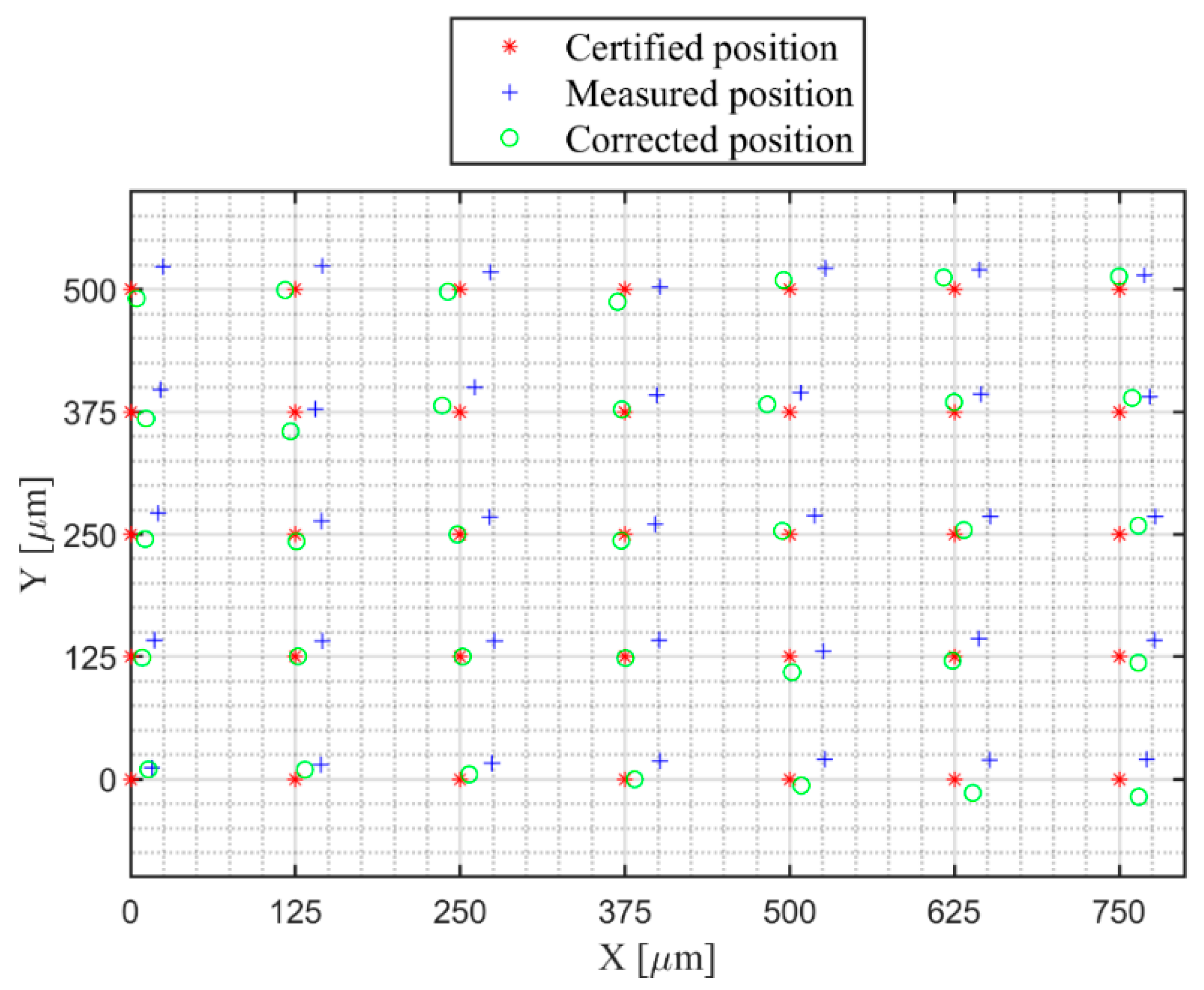
| Point No. i | Errc(i) [μm] | Errm(i) [μm] | Diff(i) [μm] | Point No. i | Errc(i) [μm] | Errm(i) [μm] | Diff(i) [μm] |
|---|---|---|---|---|---|---|---|
| 1 | 0 | 0 | 0 | 19 | 4.66 | 7.65 | −2.99 |
| 2 | 2.92 | 4.35 | −1.43 | 20 | 4.72 | 12.64 | −7.93 |
| 3 | 4.87 | 9.20 | −4.31 | 21 | 4.16 | 13.09 | −8.94 |
| 4 | 6.36 | 12.48 | −6.12 | 22 | 8.26 | 13.13 | −4.87 |
| 5 | 5.55 | 13.25 | −7.70 | 23 | 12.87 | 9.05 | 3.82 |
| 6 | 5.27 | 13.13 | −7.86 | 24 | 13.52 | 13.92 | −0.41 |
| 7 | 2.63 | 9.64 | −7.01 | 25 | 3.56 | 9.58 | −6.01 |
| 8 | 3.08 | 5.16 | −2.08 | 26 | 14.17 | 11.12 | 3.04 |
| 9 | 2.86 | 5.85 | −2.99 | 27 | 3.39 | 7.24 | −3.86 |
| 10 | 5.36 | 10.66 | −5.31 | 28 | 1.61 | 8.03 | −6.43 |
| 11 | 4.63 | 11.28 | −6.65 | 29 | 7.47 | 13.86 | −6.39 |
| 12 | 11.90 | 11.32 | 0.59 | 30 | 3.73 | 13.14 | −9.41 |
| 13 | 4.17 | 7.38 | −3.20 | 31 | 2.88 | 8.69 | −5.81 |
| 14 | 3.82 | 11.99 | −8.17 | 32 | 15.93 | 13.78 | 2.15 |
| 15 | 7.19 | 10.38 | −3.20 | 33 | 6.59 | 14.88 | −8.28 |
| 16 | 0.62 | 3.85 | −3.23 | 34 | 4.15 | 8.68 | −4.53 |
| 17 | 3.99 | 8.23 | −4.25 | 35 | 4.49 | 3.82 | 0.67 |
| 18 | 4.72 | 7.36 | −2.64 | - | |||
| mean error [μm] | 5.60 | 9.65 | |||||
| Sum of Squared error [μm2] | 1587.99 | 3684.85 |
| Simulation | No. 1 | No. 2 | No. 3 | No. 4 | No. 5 | No. 6 | No. 7 | No. 8 | No. 9 | No. 10 |
|---|---|---|---|---|---|---|---|---|---|---|
| X [μm] | −20 | −16 | −12 | −8 | −4 | 0 | 4 | 8 | 12 | 16 |
| Y [μm] | −15 | −12 | −9 | −6 | −3 | 0 | 3 | 6 | 9 | 12 |
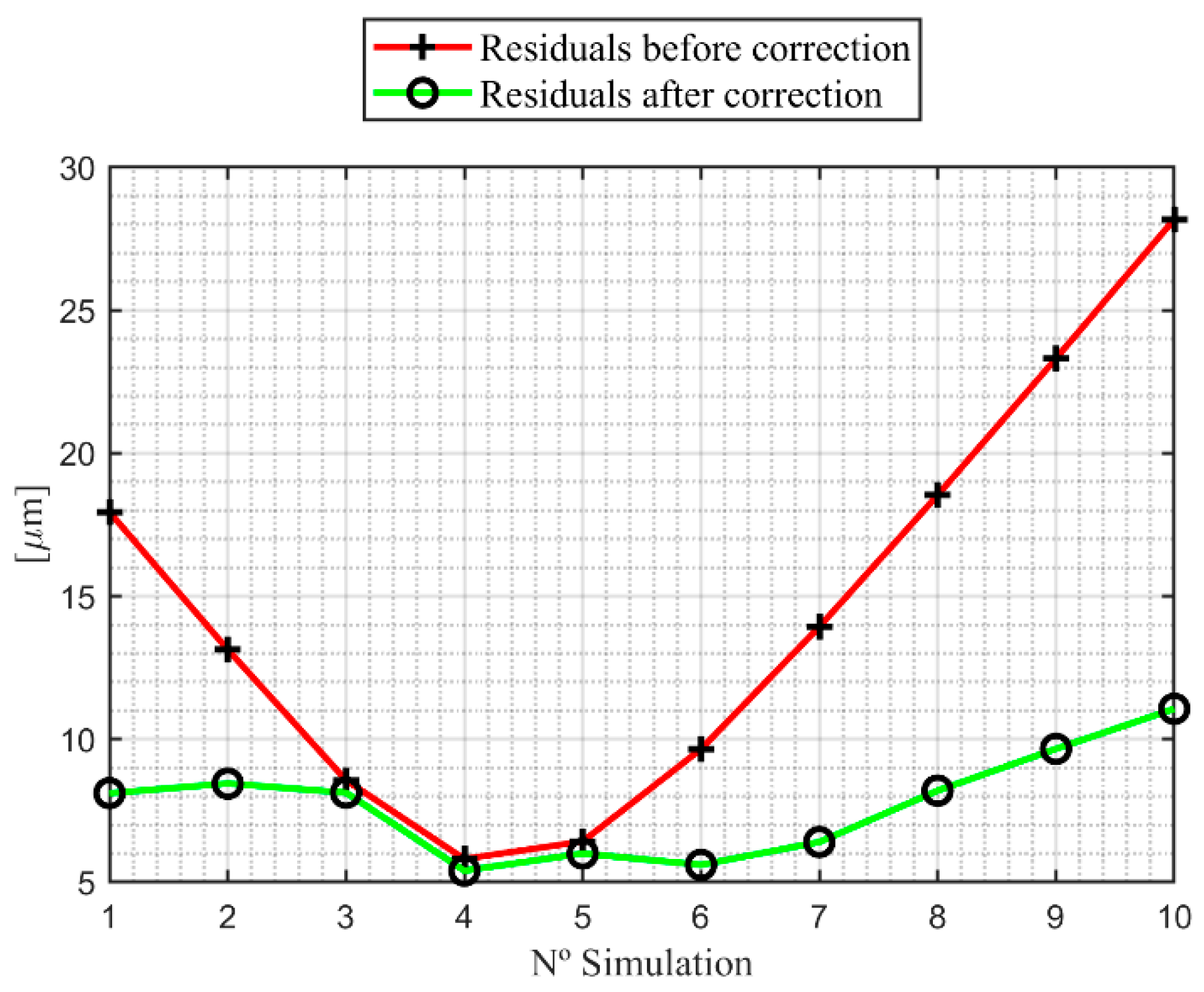
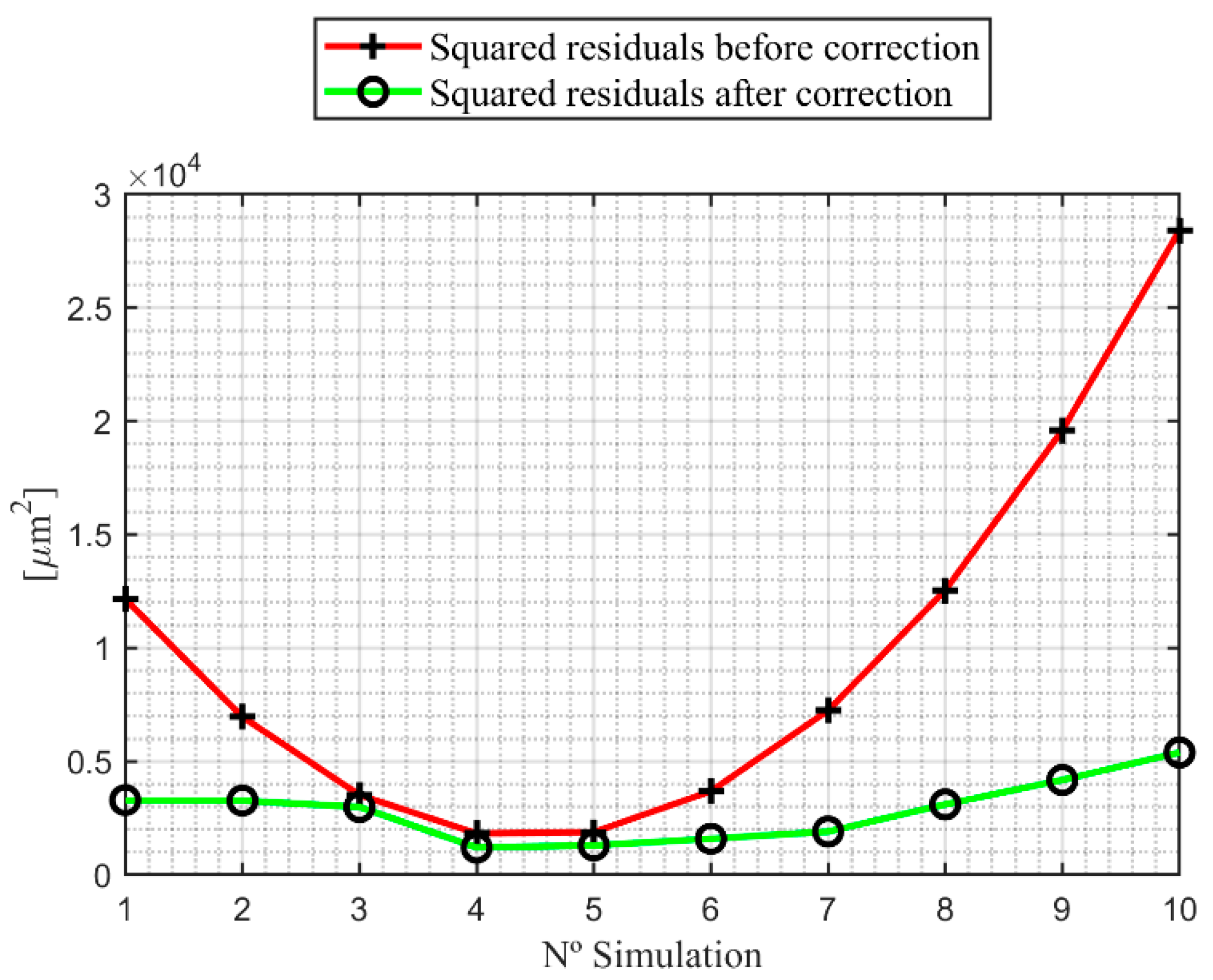
| No. Simulation | Mean Residuals [μm] | Squared Residuals [μm2] | ||
|---|---|---|---|---|
| Measured | Corrected | Measured | Corrected | |
| 1 | 17.94 | 8.11 | 12155.65 | 3287.68 |
| 2 | 13.13 | 8.45 | 6961.49 | 3269.41 |
| 3 | 8.56 | 8.13 | 3517.33 | 2986.80 |
| 4 | 5.81 | 5.23 | 1823.17 | 1206.33 |
| 5 | 6.42 | 5.96 | 1879.01 | 1288.29 |
| 6 | 9.65 | 5.60 | 3684.85 | 1587.99 |
| 7 | 13.93 | 6.40 | 7240.69 | 1903.75 |
| 8 | 18.53 | 8.20 | 12546.53 | 3101.98 |
| 9 | 23.31 | 9.66 | 19602.37 | 4179.53 |
| 10 | 28.18 | 11.06 | 28408.21 | 5389.67 |
© 2019 by the authors. Licensee MDPI, Basel, Switzerland. This article is an open access article distributed under the terms and conditions of the Creative Commons Attribution (CC BY) license (http://creativecommons.org/licenses/by/4.0/).
Share and Cite
Wang, C.; Gómez, E.; Yu, Y. Characterization and Correction of the Geometric Errors in Using Confocal Microscope for Extended Topography Measurement. Part I: Models, Algorithms Development and Validation. Electronics 2019, 8, 733. https://0-doi-org.brum.beds.ac.uk/10.3390/electronics8070733
Wang C, Gómez E, Yu Y. Characterization and Correction of the Geometric Errors in Using Confocal Microscope for Extended Topography Measurement. Part I: Models, Algorithms Development and Validation. Electronics. 2019; 8(7):733. https://0-doi-org.brum.beds.ac.uk/10.3390/electronics8070733
Chicago/Turabian StyleWang, Chen, Emilio Gómez, and Yingjie Yu. 2019. "Characterization and Correction of the Geometric Errors in Using Confocal Microscope for Extended Topography Measurement. Part I: Models, Algorithms Development and Validation" Electronics 8, no. 7: 733. https://0-doi-org.brum.beds.ac.uk/10.3390/electronics8070733