Article

Multivariate Temporal Convolutional Network: A Deep Neural Networks Approach for Multivariate Time Series Forecasting

1
Nano-Optical Material and Storage Device Research Center, School of Electronic and Electrical Engineering, Wuhan Textile University, Wuhan 430200, China
2
State Key Laboratory of Powder Metallurgy, School of Physics and Electronics, Central South University, Changsha 410083, China
*
Author to whom correspondence should be addressed.
Submission received: 7 July 2019 / Revised: 2 August 2019 / Accepted: 5 August 2019 / Published: 7 August 2019

Abstract

:
Multivariable time series prediction has been widely studied in power energy, aerology, meteorology, finance, transportation, etc. Traditional modeling methods have complex patterns and are inefficient to capture long-term multivariate dependencies of data for desired forecasting accuracy. To address such concerns, various deep learning models based on Recurrent Neural Network (RNN) and Convolutional Neural Network (CNN) methods are proposed. To improve the prediction accuracy and minimize the multivariate time series data dependence for aperiodic data, in this article, Beijing PM2.5 and ISO-NE Dataset are analyzed by a novel Multivariate Temporal Convolution Network (M-TCN) model. In this model, multi-variable time series prediction is constructed as a sequence-to-sequence scenario for non-periodic datasets. The multichannel residual blocks in parallel with asymmetric structure based on deep convolution neural network is proposed. The results are compared with rich competitive algorithms of long short term memory (LSTM), convolutional LSTM (ConvLSTM), Temporal Convolution Network (TCN) and Multivariate Attention LSTM-FCN (MALSTM-FCN), which indicate significant improvement of prediction accuracy, robust and generalization of our model.

1. Introduction

With the explosive growth of Internet of Things (IoT) applications and big data, multivariate time series is becoming ubiquitous in many fields, e.g., aerology [1], meteorology [2], environment [3], multimedia [4], power energy [5], finance [6], and transportation [7]. The precise trend forecasting, as well as for potential hazardous events, based on historical dynamical data are a major challenge, especially for aperiodic multivariate time series. One of the crucial reasons is aperiodic and nonlinearity among variables, which is incapable by models to capture and have self-adaption of the complex data features. Traditional methods such as Autoregressive (AR) [8] models and Gaussian Process (GP) [9] may fail. As an important part of the field of artificial intelligence, deep neural networks (DNNs) provide state-of-the-art accuracy on many tasks [10] and has been developed intensively in natural language processing (NLP), computer vision (CV), time series classifications and time series forecasting.
Enlightened by algorithms used in NLP (i.e., Sequence to Sequence [11,12] and Attention mechanism) and CV (i.e., Dilated convolution network [13] and residual structure [14]), in this paper, the M-TCN model is proposed for aperiodic multivariate time-series prediction, which constructs the aperiodic data as sequence-to-sequence and a novel multichannel and asymmetric residual blocks network. The model is cross validated by a rich set of existing competitive models with an aperiodic time series dataset. The reminder of the article is organized as follows: Section 2 reviews the background work. Section 3 presents the methodology of the proposed model. In Section 4, the experiment is analyzed and discussed. Finally, conclusions and outlook are drawn in Section 5.

2. Background

One of the major challenges of multivariate time series forecasting is nonlinearity and aperiodic of data originated by short-term and long-term dynamical behavior. Various models have been established based on classical statistic methods or machine learning algorithms.
The prominent classical univariate time series model is Autoregressive (AR) with classical statistic algorithms, as well as its progeny. The AR method is well used to stationary time series. The improved models, such as autoregressive integrated moving average (ARIMA) [15], autoregressive moving average (ARMA) [16], and vector auto-regression (VAR) [17], were developed by including flexible exponential smoothing techniques. However, for long-term temporal patterns, these models are inevitably prone to overfitting and high computational cost, especially for high-dimensional inputs.
Alternative methods by treating the time series forecasting problems as general regression with time-varying parameters were applied by machine learning models, e.g., linear support vector regression (SVR) [18], random forest [19], ridge regression [20] and LASSO [21] models. Those models are practically more efficient due to high quality off-the-shelf solutions in machine learning community. Still, machine learning based models may be incapable of including complex nonlinearity dependences of multivariate large datasets.
Meanwhile, the well-built deep neural networks of Convolutional Neural Networks (CNNs) and Recurrent Neural Networks (RNNs) have been widely applied in time series forecasting, which are attributed to the open source deep learning frameworks, such as Keras (Keras, available online: https://keras.io), TensorFlow (TensorFlow, available online: https://tensorflow.org) and PyTorch (PyTorch, available online: https://pytorch.org), including flexible and sophisticated mathematical libraries. Some representative models are long short-term memory (LSTM) [22] and its inheritors, convolutional LSTM (ConvLSTM) [23] and Multivariate Attention LSTM-FCN (MALSTM-FCN) [24], which overcome the challenges involved in training a recurrent neural network for a mixture of long and short-term horizons. However, these models are time consuming and non-robust for aperiodic data forecasting.
Another novel method for time-series forecasting is a hybrid multiscale approach, such as empirical mode decomposition (EMD) [25], ensemble EMD (EEMD) [26], multi-level wavelet decomposition network (mWDN) [27] and variational mode decomposition (VMD) [28]. These methods are used to decompose data into different frequencies’ components to facilitate forecasting. However, the pre-design decomposition K value is an essential prerequisite as an input of training models, which is not versatile for complicated multivariate time series prediction.
Recently, a general architecture for a predictive sequences model by convolutional and recurrent architecture on sequence modeling tasks, the Temporal Convolution Network (TCN) [29], is proposed. The prominent characteristics of TCNs are casualness in convolution architecture design and sequence length. In addition, it is also convenient to build a very deep and wide network by a combination of residual network and extended convolution. Under this background, our model is designed based on TCN and tested for PM2.5 and electric power forecasting.
For comparison, Table 1 contrasts the advantages and challenges of some common methods for multivariate time series prediction.

3. Methodology

In this section, the time series forecasting problem is formulated first. In addition, then the baseline models, ConvLSTM and Multivariate LSTM FCN are presented to be used as the methods in our comparative evaluation. Finally, M-TCN model is introduced.

3.1. Sequence Problem Statement

From the nature of machine learning, to minimize the expected error, it requires obtaining an ideal nonlinear mapping from a historical dataset to a current state, especially for hazard events forecasting. The prerequisite is to employ enough characteristic parameters to feature the various phenomena, which makes the current state strictly dependent on the historical dataset. The problem of multivariable time series prediction is defined as the problem of sequence to sequence in this paper. Before defining the network structure, more formally, given an input sequence time series signal X = x 1 , x 2 , , x T with x t R n , where n is the variable dimension, we aim at predicting corresponding outputs Y = y 1 , y 2 , , y h at each time. The target of sequence modeling network is to obtain a nonlinear mapping to the prediction sequence from the current state as:
y 1 , y 2 , , y h = f x 1 , x 2 , , x T .

3.2. Baseline Test

To build a baseline test benchmark, the traditional models, naive forecast, average approach forecast and seasonal persistent forecast models are included for a cross evaluation.
Naive forecast model: It takes the value from the last hour prior to the forecast period (e.g., 24 h) and uses it as the value of a dataset for each hour in the forecast period (e.g., 1 to 24 h). Using the naive approach, forecasts are produced that are equal to the last observed value. This model is defined as:
y ^ T + 1 = y T ,
where y T is the past data, and y ^ T + 1 is the next time value.
Average approach forecast model: In this model, the predictions of all future values are equal to the mean of the past data. This method can be used for any type of data available in the past and defined as:
y ^ T + 1 = y ¯ = y 1 + + y T / T ,
where y 1 , y 2 , , y T is the past data, and y ^ T + 1 is the next time predicted value.
Seasonal persistent forecast model: It defines the same time period a year ago as the predicted value. This method accounts for seasonality by setting each prediction to be equal to the last observed value of the same season. This model is defined as:
y ^ T + 1 = y T Y ,
where y T Y is the past data, and y ^ T + 1 is the next time predicted value.

3.3. ConvLSTM Encoder–Decoder Model

A convolutional LSTM (ConvLSTM) encoder–decoder network is built in this work, which reconstructs the input sequence and predicts the future sequence simultaneously. The ConvLSTM input layer is designed to be a 4D tensor [timestep, row, column, channel], where timestep is the number of subsequences, row is the one-dimensional shape of each subsequence, column is the hours in each subsequence and channel is the features that we are working with as input. The encoding ConvLSTM compresses the whole input sequence into a hidden state tensor and the decoding LSTM unfolds this hidden state to give the final prediction. An overview of the ConvLSTM is shown in Figure 1.
Multivariate ALSTM Fully Convolutional Networks models are comprised of temporal convolutional blocks and an LSTM block, as depicted in Figure 2. The feature extractor consists of three stacked temporal convolutional blocks. In addition, the first two convolutional blocks conclude with a squeeze and excite block.
We consider this model structure as a parallel structure of CNN (temporal convolutional blocks) and RNN (LSTM block). In order to study the regression problem, the final softmax layer used for classification is changed to a fully connected layer with 24 nodes.

3.4. M-TCN Model

The main characteristic of CNN is a local feature by convolving filters. For time series forecasting, the local correlation is reflected in the continuous change over a period of time within a small time slot. In addition, RNN models, such as LSTM, have always been considered as the best standard method to solve sequence problems; however, RNNs cannot be parallel, resulting in huge time-consumption compared to that of CNN. From those considerations, the overall framework of the model is designed based on CNN. Our aim is to distill the best practices in designing convolutional networks to be flexible and stable frameworks with a simple architecture and high efficiency for multivariate time series forecasting. The distinguishing characteristics of M-TCN are: (1) the input and output lengths of our network could be determined to be flexible for various scenarios; (2) M-TCN uses the 1D convolution instead of causal convolutions; (3) M-TCN augmented with two different asymmetric residual blocks; (4) M-TCN constructs a sub-model for each feature of input data, and the prediction is accomplished by a combination of all sub-models. We call this typical structure a multihead model. In this work, what we emphasize is the methodology on how to build effective networks (i.e., Multihead model) using a combination of network (augmented with two different residual blocks) and dilated convolutions. The following are details of the network structure.

3.4.1. 1D Convolutions

TCN uses causal convolutions, where an output at time t is convolved only with elements from time t and earlier in the previous layer. In Figure 3, causal convolution is used to assume that all data must have a one-to-one causal relationship in chronological order. Given an input sequence time series signal X = x 1 , x 2 , x 3 , x 4 , x 5 with x t R n where n is the variable dimension, x t does not strict causality in chronological order. While x 1 and x 5 may have a direct logical connection, causal convolution will make the relationship between x 1 and x 5 affected by x 2 , x 3 , x 4 . This design was limited by the absolute order of time-series and inefficient for accurate characteristics learning at a relative time. Thus, in our model, only a 1D convolutional network is adopted to avoid this situation.

3.4.2. Dilated Convolutions

The dilated convolutions algorithm [13] is used in our model. Since the traditional convolution operation process is to convolute the sequence once and then pool, which reduces the size of the sequence and enlarges the receptive field at the same time. One of the main faults is that some sequential information will be lost during the pooling process, while the advantage of dilated convolutions is that they don’t need the pooling process and gradually increase the field of perception through a series of dilated convolutions, thus leading to the output of each convolution encompasses rich information for long-term tracking. Thus, the dilated convolutions could be well applied in the problem of long information dependence of sequence, such as voice and signal processing, environment forecasting, etc. Dilated convolution is defined as
F ( s ) = x d f ( s ) = i = 0 k 1 f ( i ) · x s d · i ,
where d is the dilation factor, k is the filter size, and s d · i accounts for the direction of the past. A filter f : { 0 , , k 1 } N . Figure 4 depicts dilated 1D convolutions for dilations 1, 2 and 4.

3.4.3. Residual Block

A novel structure is designed by a multilayer and sequential residual network and parallel residual blocks. The core of ResNet [14] is to create a shortcut for information dissemination in front and back layers. A basic Residual block is used in the TCN network; however, the jump connection in ResNet, resulting in only a small number of residual blocks’ learning useful information, and thus the basic residual block structure is not adapted for time series prediction. An alternative way is to increase the convolution kernel size for a better prediction; however, the computational load increases sharply. In [31], an asymmetric block structures were introduced both for MobileNetV3-Large and MobileNetV3-Small. By this way, asymmetric factors will be generated in the whole network structure and may make a positive impact on the in-depth learning models. The optimal asymmetric structure needs Neural Architecture Search(NAS) [32,33]; however, it is computationally expensive. In a more direct way, two asymmetric residual blocks in parallel are constructed. The architectural elements in our model are shown in Figure 5.
The Unit for our model is shown in Figure 5 (left). The Unit has two channels. Each channel has dilated convolution and nonlinearity, for which we used the rectified linear unit (ReLU) [34]. The residual block 1 is shown in Figure 5 (middle). Within a residual block, the model has three units. The output is the sum of the results of two channel operations. The residual block 2 is shown in Figure 5 (right), which has the same basic structure as residual block 1, but one more unit layer is implemented. To be more precise, a dilated convolution with different dilation factors and filter size k = 3 are constructed both for residual blocks. In addition, an optional 1 × 1 convolution is introduced to adjust the dimensions of different feature maps (see Figure 5 (middle, right)) for summation.
The Unit takes the same input with two different convolutions, and then adds up the results. The convolutional layer consists of multiple kernels with different sizes. The k-th filter sweeps through the input data X, which can be formulated as:
ReLU ( x ) = max ( 0 , x ) ,
h 1 k = ReLU W k X + b k ,
h 2 k = ReLU W k X + b k ,
h k = h 1 k + h 2 k ,
where h 1 k is the result of channel 1, h 2 k is the result of channel 2, and h k is result of unit. * stands for a convolutional operation.
A residual block contains a channel, which passes through a series of conversion functions F , and the final output is added to the input X of the block:
o = ( x + F ( x ) ) .

3.4.4. Fully Connected Layers

Fully connected layers can be replaced by global average pooling (GAP) for better efficiency and accuracy in image recognition tasks. However, fully connected layers are essential in prediction tasks and can easily change the length of the output sequence. Formally, a statistic z R C is generated by shrinking X through its spatial dimensions H × W , such that the output z is calculated by:
z = G A P x c = 1 H × W i = 1 H j = 1 W x c ( i , j ) .
The whole spatial feature on a channel is averaged as a global feature. Each feature map is averaged into one value, thus the local information of the whole feature value is lost, which has a negative impact on the prediction problem.
The full connection layer is shown in Figure 6, which not only establishes the position relationship between feature maps, but also retains the internal feature information of the same feature map. This will have a beneficial impact on the prediction problem. The disadvantage is that the parameters are greatly increased.

3.4.5. Multi-Head Model

The model is further extended so that each input variable has a separate sub-model, named after a multi-headed model. This sub-model for each input variable has to be defined first. Each sub-model learns the information with different features in the sequence separately. In addition, the outputs of those models are then combined in series to form a very long vector, which is interpreted by some fully connected layers before the prediction is made. An overview of multi-head temporal convolutional network (M-TCN) architecture is shown in Figure 7. To provide more detail, an overview of convolutions is shown in Figure 8.

3.5. Training Procedure

The training procedure can be described as Algorithm 1.
Meaning represented by each parameter. m i n _ l r : minimum learning rate; i n i t i a l _ l r : initial learning rate; factor: factor by which the learning rate will be reduced; wait: number of epochs with no improvement after which learning rate will be reduced; n e w _ l r : new learning rate; epoch: number of epochs to train the model; b e s t _ s c o r e : minimum RMSE.
Algorithm 1: Training procedure.
1:
m i n _ l r = 1e-4; epoch = 200; i n i t i a l _ l r = i n i t i a l _ l r
2:
factor
3:
for n < epoch do
4:
 wait += 1
5:
 if b e s t _ s c o r e > RMSE
6:
    b e s t _ s c o r e = RMSE
7:
   save model
8:
   if wait >= 10
9:
   if i n i t i a l _ l r > m i n _ l r
10:
     m i n _ l r = i n i t i a l _ l r × factor
11:
     n e w _ l r = max( n e w _ l r , m i n _ l r )
12:
    wait = 0

4. Experiments

In this section, we first describe two datasets for empirical studies. All of the data are available online. Then, the parameter settings of model and evaluation metrics are introduced in our studies. Finally, the proposed M-TCN model against different baseline models is compared.

4.1. Datasets

Two benchmark datasets are used which are publicly available. Table 2 summarizes the corpus statistics.
Beijing PM2.5 Dataset (available online: https://archive.ics.uci.edu/ml/datasets/Beijing+PM2.5+Data): It contains hourly PM2.5 data and the associated meteorological data in Beijing, China. The exogenous time series include dew point, temperature, and atmospheric pressure, combined wind direction, cumulated wind speed, hours of snow, and hours of rain. In total, we have 43,824 multivariable sequences. For this dataset, the hourly PM2.5 data are used as a predictive value.
ISO-NE Dataset (available online: https://www.iso-ne.com/isoexpress/web/reports/load-and-demand): The time range of the dataset is between March 2003 and December 2014. The ISO-NE Dataset includes hourly demand, prices, weather data and system load. The dataset contains two variables, which are hourly electricity demand in MW and dry-bulb temperature in F. For this dataset, the hourly electricity demand is used as a predictive value.
In our experiments, ISO-NE datasets have been split into training set (from 1 March 2003 to 31 December 2012), valid set (the whole year of 2013) and test set (the whole year of 2014) in a chronological order. In addition, the Beijing PM2.5 Dataset has been split into a training set (from January 2, 2010 to December 31, 2012), valid set (the whole year of 2013) and test set (the whole year of 2014) in a chronological order.

4.2. Data Processing

According to the characteristics of each dataset, it is necessary to preprocess the data. Each of the datasets is normalized with a mean of 0 and a standard deviation of 1.
For the Beijing PM2.5 Dataset, PM2.5 is NA in the first 24 h. We will, therefore, need to remove the first row of data. There are also a few scattered “NA” values later in the dataset, and we use zero to fill in missing values. The wind speed feature is label encoded (integer encoded). We apply the new dataset to every algorithm in later experiments.

4.3. Evaluation Criteria

Three evaluation metrics, root mean squared error (RMSE), root relative squared error (RRSE) and empirical correlation coefficient (CORR) for multivariate forecasting, are used and defined as:
RMSE = 1 N i = 1 N y t i y ^ t i 2 ,
RRSE = ( i , t ) Ω T e s t ( Y i t Y ^ i t ) 2 ( i , t ) Ω T e s t ( Y i t mean ( Y ) ) 2 ,
CORR = 1 n i = 1 n t ( Y i t mean ( Y i ) ) ( Y ^ i t mean ( Y ^ i ) ) t ( Y i t mean ( Y i ) ) 2 ( Y ^ i t mean ( Y ^ i ) ) 2 ,
where Y , Y ^ R n × T are ground value and system prediction value, respectively, and Ω Test is the set of time stamps used for testing. For RMSE and RRSE, the lower value is better, while, for CORR, the higher value is better for evaluation.

4.4. Walk-Forward Validation

In the test set, the Walk-Forward Validation method is adopted, but the model is not updated. In this case, a model is needed to predict a period of time, and then the actual data of the current period is provided to the model, so that it can be used as the basis for the prediction of subsequent periods. This is not only applicable to the way the model is used in practice, but also conducive to the model using the best available data.
In the experiment, the output length is set to 24. For multi-step prediction problems, we evaluate each prediction time step separately. Table 3 summarizes the actual value and predicted value. Models can be trained and evaluated as follows.
  • Step 1: Starting at the beginning of the test set, the last set of observations in the training set is used as input of the model to predict the next set of data (the first set of true values in the validation set).
  • Step 2: The model makes a prediction for the next time step.
  • Step 3: Get real observation and add to history for predicting the next time.
  • Step 4: The prediction is stored and evaluated against the real observation.
  • Step 5: Go to step 1.

4.5. Experimental Details

To be more specific, most models chose input length from { 24 , 72 , 168 } , and the batch size is set to 100. The mean squared error is the default loss function for forecasting tasks. Adam [35] is adopted as optimization strategy, with an initial learning rate set to 0.001. In addition, the learning rate is reduced by a factor of every 10 epochs of no improvement in the validation score, until the final learning rate was reached.
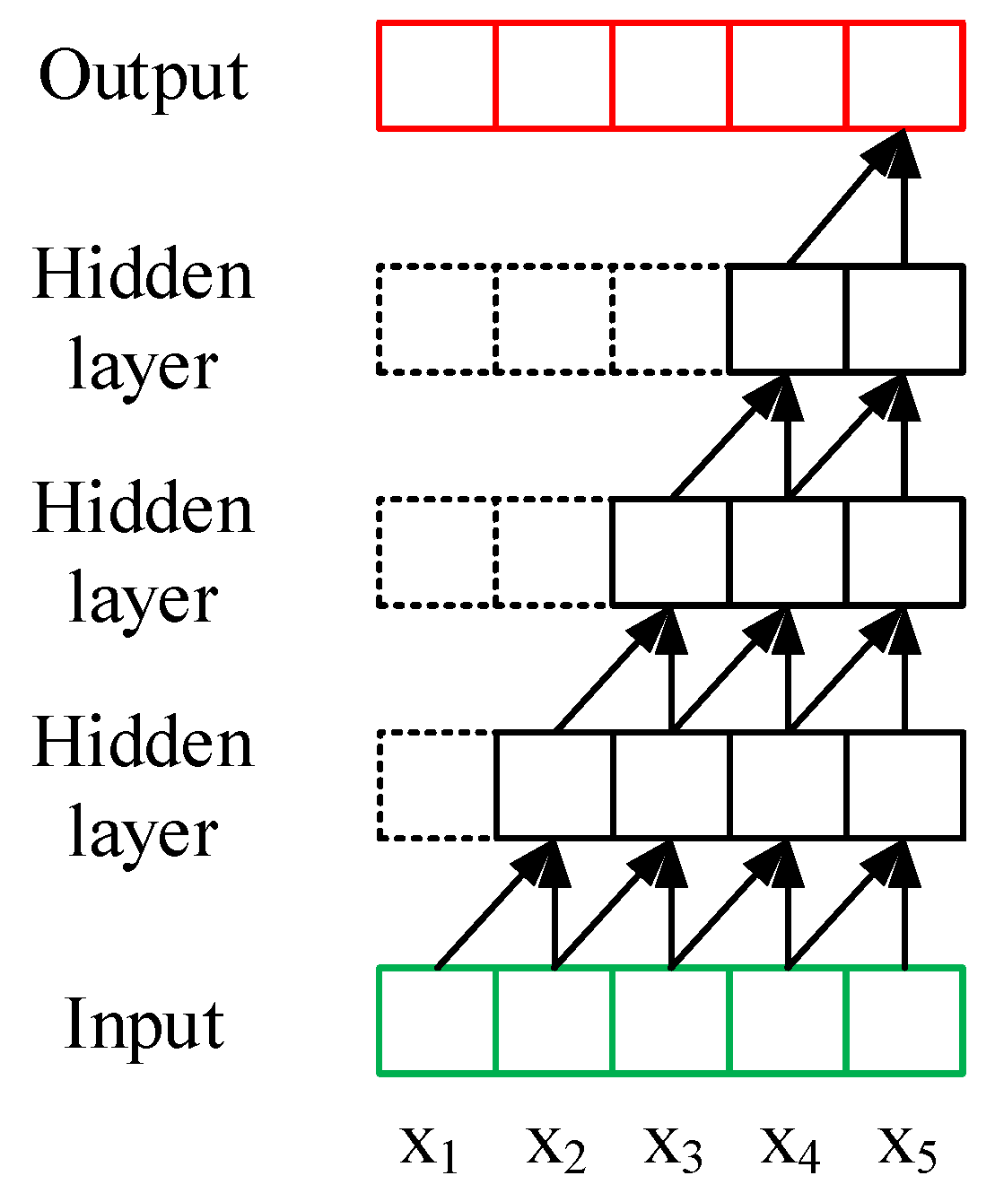
For the LSTM model, a single hidden layer with { 50 , 100 , 200 } units is defined. The number of units in the hidden layer is unrelated to the number of time steps in the input sequences. Finally, an output layer will directly predict a vector with 24 elements, one for each hour in the output sequence. SGD [36] is adopted as an optimizer. The learning rate is set to 0.05 with a reduction rate by a factor of 0.3.
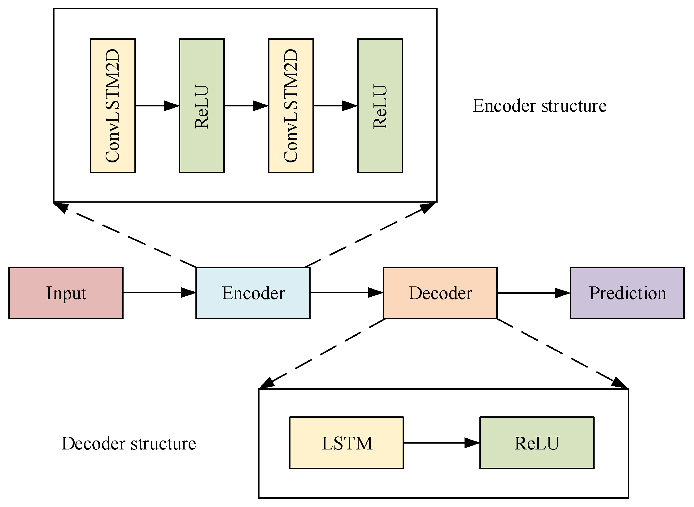
In the ConvLSTM Encoder–Decoder model, input data have the shape of [timestep, row, column, channel]. Timestep is chosen from { 1 , 3 , 7 } . Row is set to 1. Column is chosen from { 24 , 72 , 168 } . Channel is chosen from { 2 , 8 } . SGD is adopted as the optimization algorithm. The learning rate is set as the same in LSTM. For this network, the 1-layer network contains one ConvLSTM layer with 64 hidden states, the 2-layer network contains one ConvLSTM layer with 128 hidden states, and the 3-layer network has 200 hidden states in the LSTM layers. All the input-to-state and state-to-state kernels are of size 1 × 3 .
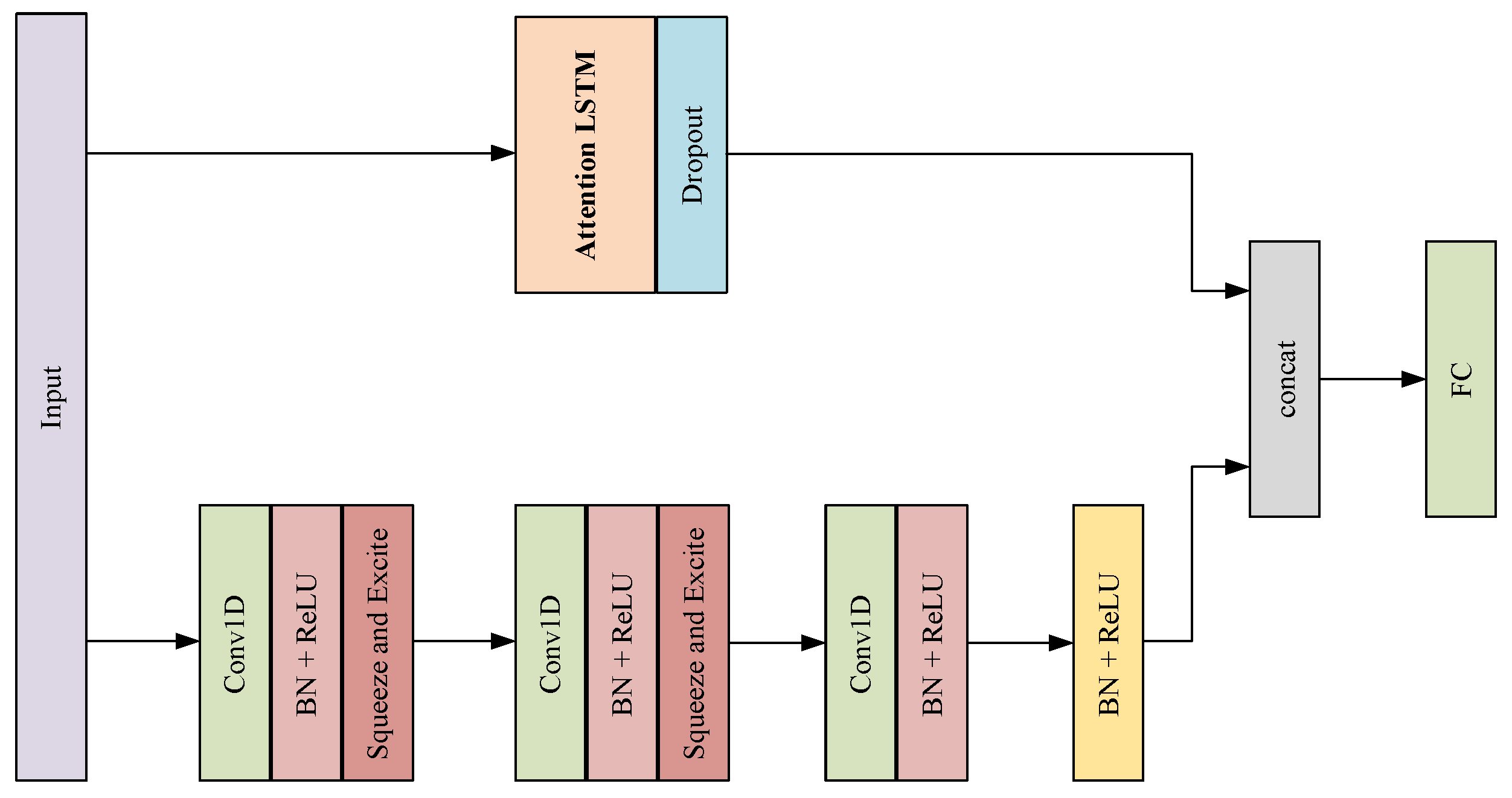
For the MALSTM-FCN network, the optimal number of LSTM hidden states for each dataset was found via grid search over { 8 , 50 , 100 , 200 } . The FCN block is comprised of three blocks of 128-256-128 filters. The models are trained using a batch size of 128. The convolution kernels are initialized following the work of [24].
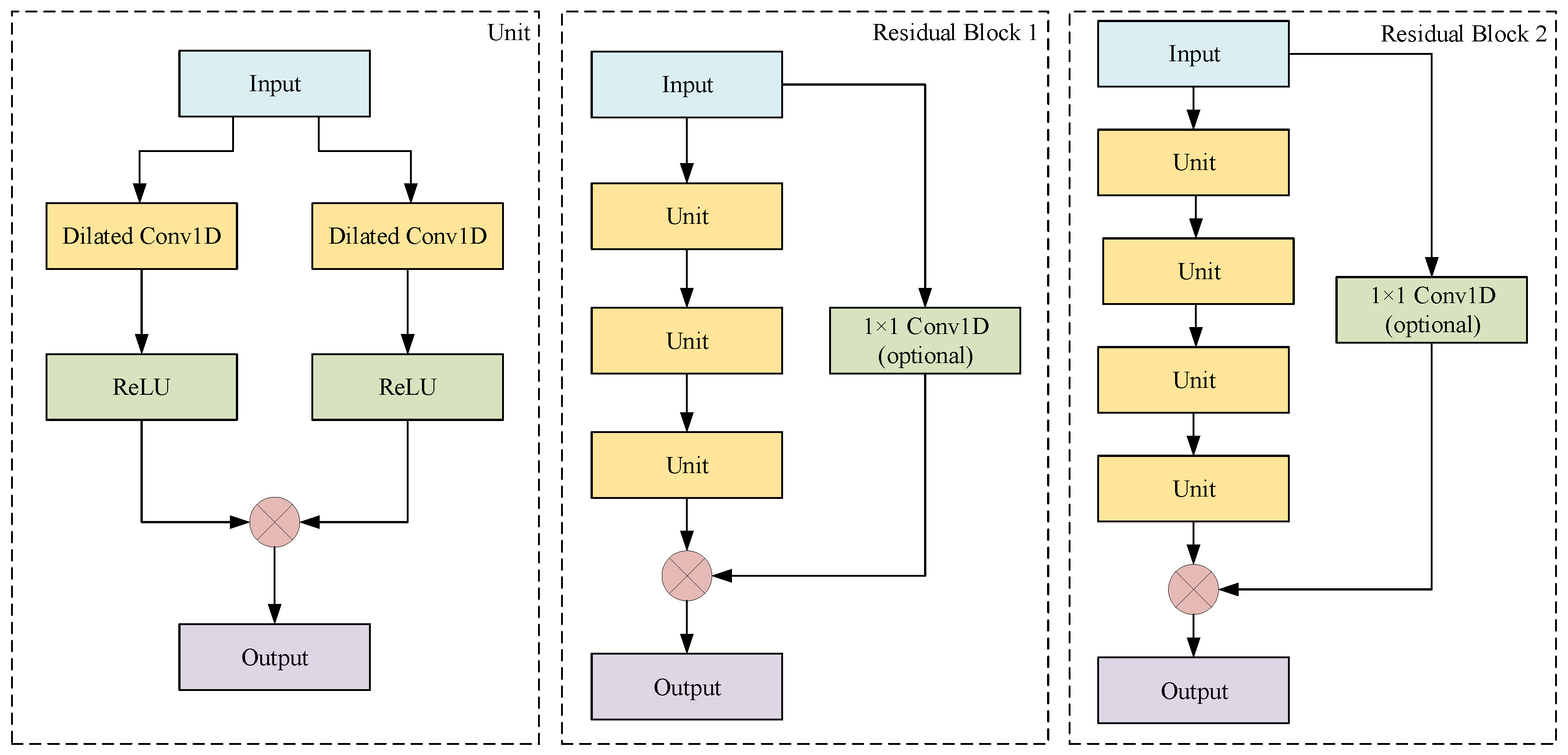
For the TCN network, the optimal number of hidden units per layer for each dataset was found via grid search over { 30 , 50 , 100 } . The convolution kernels are of size 1 × 3 .
In our M-TCN model, Adam is adopted as an optimization strategy with an initial learning rate set to 0.001(ISO-NE Dataset), while, for Beijing PM2.5, SGD is adopted as an optimization strategy with an initial learning rate set to 0.05.
The implementations of M-TCN are built based on Keras library with the Tensorflow backend. We run all the experiments on a computer with a single NVIDIA 1080 GPU (Santa Clara, CA, USA).

4.6. Experimental Results

Table 4 summarizes the results on multivariate testing sets in the metrics RMSE, RRSE and CORR across all forecast hours. The output sequence length is set to 24, which means that the horizons were set from the 1st hour to the 24th hour for forecasting over the Beijing PM2.5 and ISO-NE Electricity data. In the time series forecasting, larger horizons shall make the prediction harder. Thus, our experiments give a detailed analysis of the results in this large horizon. The best results for each data and metric pair are highlighted in bold. To demonstrate the effectiveness of the models, the results are compared with three baseline methods by the Naive, Average and Seasonal persistent model, as well as four competitive algorithms of LSTM, ConvLSTM, TCN and MALSTM-FCN. For RMSE and RRSE, the lower value is better, while the higher value is better for CORR. Overall performance of neural network based models is better than traditional methods. The performance of M-TCN is comparable with LSTM and MALSTM-FCN and outperforms both of them by about 10%∼20% for both datasets. Furthermore, the ConvLSTM model has weak generalization ability, and its prediction ability varies greatly on different datasets.
Figure 9 presents the results on RMSE for both datasets at a larger horizon from the 1st hour to the 24th hour. It is obvious that M-TCN is better than others and RRSE maintains a steady increase without obvious fluctuation in the long-term forecasting period.

4.7. Spectrum Analysis

In order to further study the performance of the model, we analyzed the spectrum of the test set and the prediction data. Spectrum refers to the representation of a time domain signal in frequency domain, which can be used for discrete Fourier transform of sequence data. Discrete Fourier Transform (DFT) of k points are computed as:
X ( k ) = D F T [ X ( n ) ] = n = 0 N 1 X ( n ) W n k ( 0 k N 1 ) ,
W = e j 2 π N ,
where X ( k ) is the time series.
More detailed calculations include:
X k f 1 = D F T x n T s = n = 0 N 1 X n T s e j 2 π N n k ,
f 1 = 1 T 1 ,
T s = T 1 N ,
where T 1 is signal time, f 1 is the frequency interval, N is the number of signal sampling, and T s is the signal sampling interval time.
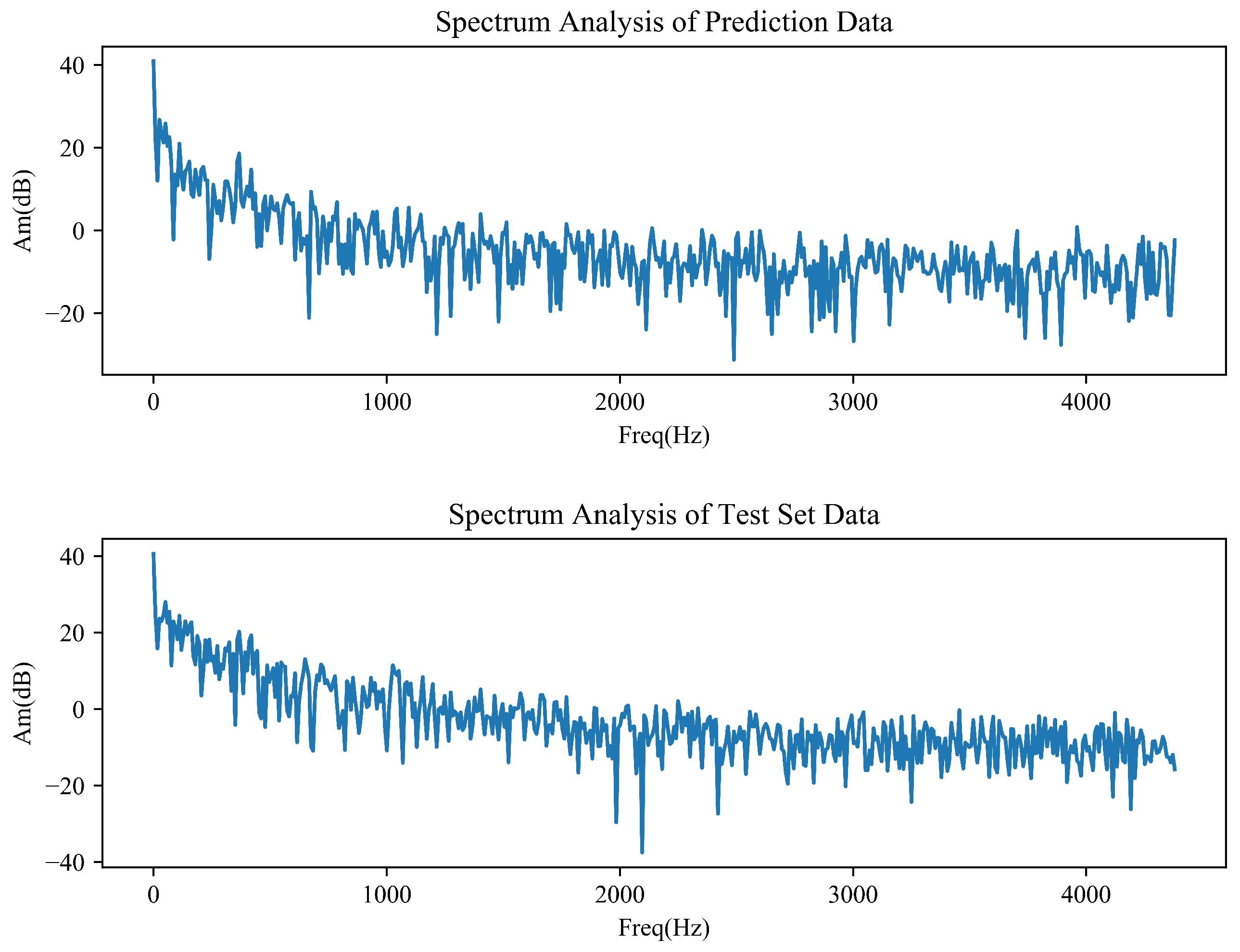
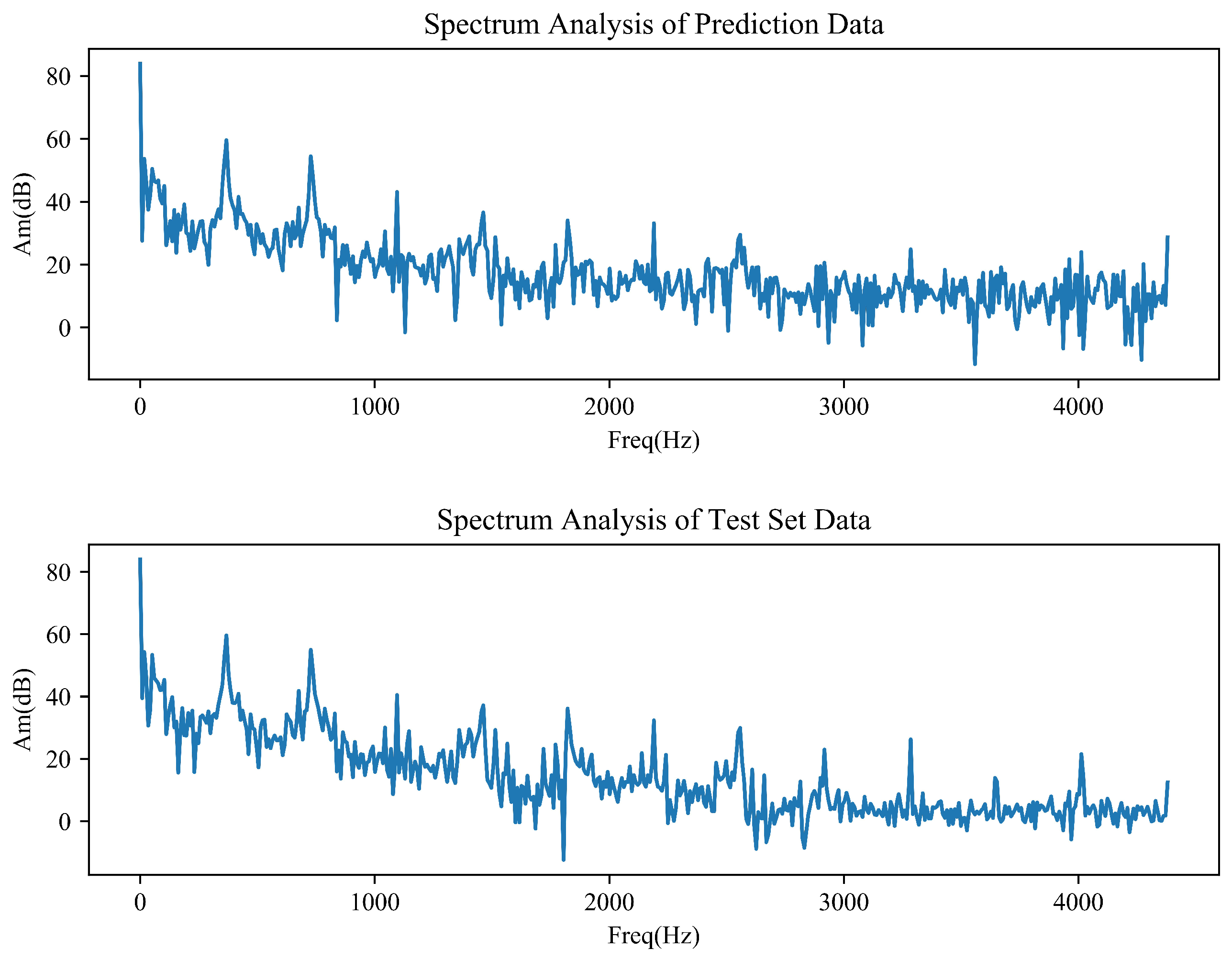
The amplitude spectrum analysis of these datasets is performed, so as to check the existence of repetitive patterns in the datasets. The hourly PM2.5 and ISO-NE data of test set and predictions are plotted in the frequency domain as shown in Figure 10 and Figure 11 separately, where Freq is the frequency with a unit of 1/Hour and Am is the amplitude in dB. Sampling frequency is set to 8760 (the same as test set time variable length). Sampling frequency is set to 8760 (the same as the time variable length set by the test), which ensures that the frequency and time correspond to each other numerically. Both figures show that frequency domain is irregular continuous waveform indicating a non-periodic of PM2.5 and ISO-NE datasets. As can be clearly seen, PM2.5 data have no periodicity, which brings great errors to accurate prediction. Since the ISO-NE data change regularly from 1 to 1000 h, the prediction effect is the best.

4.8. Ablation Tests

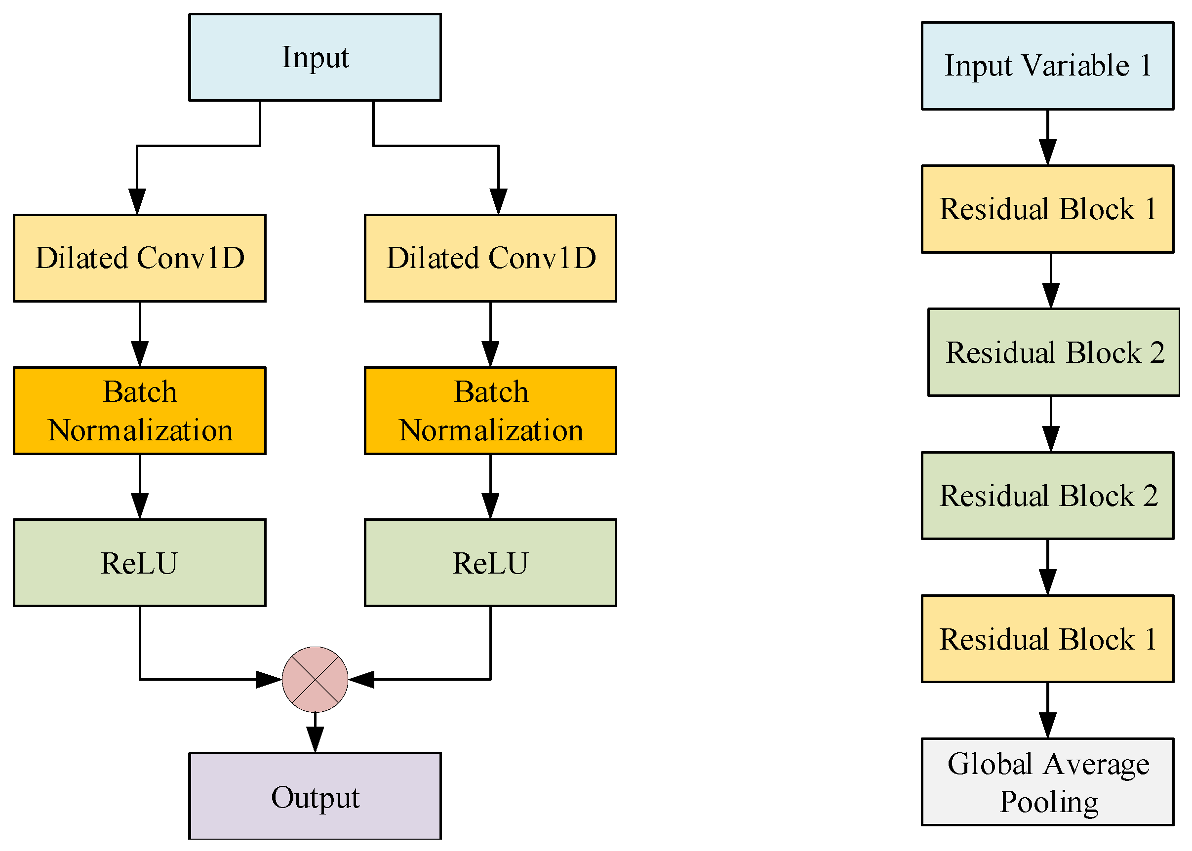
Furthermore, to demonstrate the efficiency of our model structure, a careful further study is performed. Specifically, we add each component one at a time in our framework. M-TCN with different components are defined as follows:
Model/w/BN: The model adds a Batch Normalization (BN) [37] component. In this test, Batch Normalization was applied to the input of each nonlinearity, in a convolutional way, while keeping the rest of the architecture constant. Figure 12 (left) describes this model in detail.
Model/r/GAP: In the model, the full connection layer is replaced by the global average pooling. Figure 12 (right) describes this model in detail.
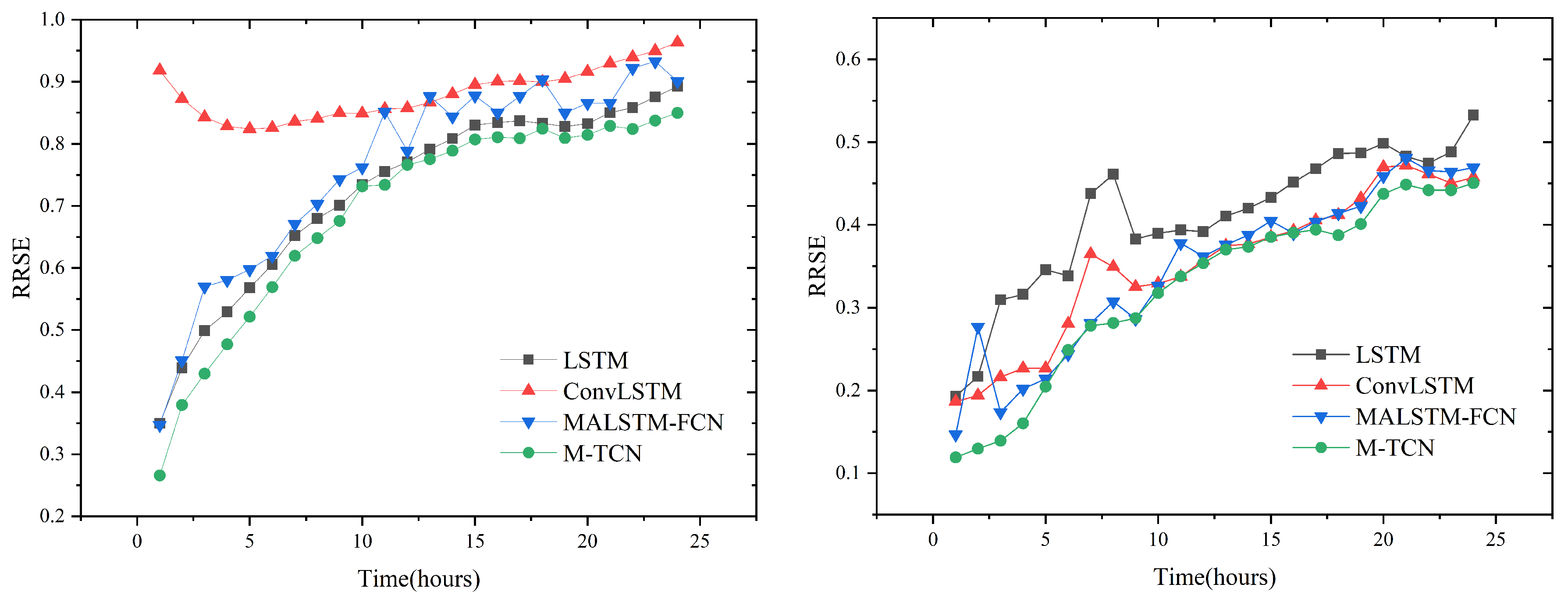
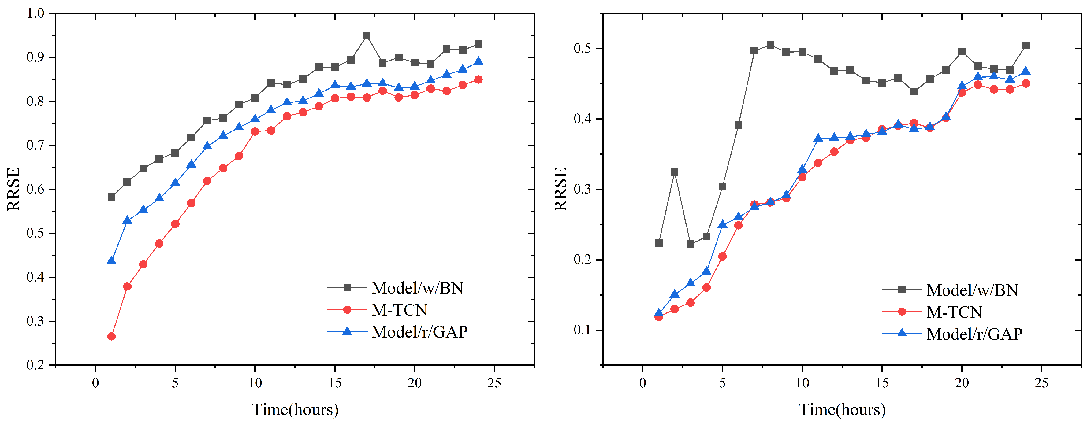
The test results measured using RRSE are shown in Figure 13. Comparing the results, we see that, in both datasets, BN cannot help the network achieve higher accuracy. Adding the BN components in (Model/w/BN) caused big performance drops on both datasets. All of the components of the M-TCN model together lead to the robust performance of our approach on the Beijing PM2.5 dataset.

4.9. Model Efficiency

s/epoch denotes the time required for each epoch (in seconds). Boldface indicates the best result. In Table 5, M-TCN proves to be quite competitive.

5. Conclusions

The multivariate time series forecasting is investigated by introducing a novel M-TCN model, in order to compare with traditional models and especially deep learning (generic recurrent architectures such as LSTM; generic convolutional architecture such as TCN; hybrid architectures such as ConvLSTM and MALSTM-FCN.). In M-TCN, the dilated network is employed as a meta-network and asymmetric residual blocks are constructed. The proposed approach significantly improved the results in time series forecasting on benchmark datasets of Beijing PM2.5 and ISO-NE. Our research focuses on the trade-off between implementation complexity and prediction accuracy. With in-depth analysis and empirical evidence, the results indicate a prominent efficiency of M-TCN.
For future research, we will focus on the extraction technology based on higher-order statistical features instead of fully connected layers, which can reduce the parameters of the model and training time.

Author Contributions

Conceptualization, R.W. and S.M.; methodology, R.W.; software, S.M.; validation, S.M. and J.W.; formal analysis, S.M.; investigation, R.W. and F.Y.; resources, M.L.; data curation, R.W. and F.Y.; writing—original draft preparation, S.M.; writing—review and editing, R.W. and F.Y.; visualization, S.M.; supervision, R.W.; project administration, F.Y.; funding acquisition, R.W. and M.L.

Funding

This work was supported by the National Natural Science Foundation of China (Grant No. 11505130 and 21872174), the Project of Innovation-Driven Plan in Central South University (2017CX003), State Key Laboratory of Powder Metallurgy, Shenzhen Science and Technology Innovation Project (JCYJ20180307151313532), Thousand Youth Talents Plan of China and Hundred Youth Talents Program of Hunan.

Conflicts of Interest

The authors declare no conflict of interest.

References

  1. Seyed, B.L.; Behrouz, M. Comparison between ANN and Decision Tree in Aerology Event Prediction. In Proceedings of the International Conference on Advanced Computer Theory & Engineering, Phuket, Thailand, 20–22 December 2008; pp. 533–537. [Google Scholar] [CrossRef]
  2. Simmonds, J.; Gómez, J.A.; Ledezma, A. Data Preprocessing to Enhance Flow Forecasting in a Tropical River Basin. In Engineering Applications of Neural Networks; Springer: Cham, Switzerland, 2017; pp. 429–440. [Google Scholar]
  3. Mohamad, S. Artificial intelligence for the prediction of water quality index in groundwater systems. Model. Earth Syst. Environ. 2016, 2, 8. [Google Scholar]
  4. Amato, F.; Castiglione, A.; Moscato, V.; Picariello, A.; Sperlì, G. Multimedia summarization using social media content. Multimed. Tools Appl. 2018, 77, 17803–17827. [Google Scholar] [CrossRef]
  5. Kadir, K.; Halim, C.; Harun, K.O.; Olcay, E.C. Modeling and prediction of Turkey’s electricity consumption using Artificial Neural Networks. Energy Convers. Manag. 2009, 50, 2719–2727. [Google Scholar]
  6. Wu, Y.; José, M.H.; Ghahramani, Z. Dynamic Covariance Models for Multivariate Financial Time Series. arXiv 2013, arXiv:1305.4268. [Google Scholar]
  7. Yu, R.; Li, Y.; Shahabi, C.; Demiryurek, U.; Liu, Y. Deep learning: A generic approach for extreme condition traffic forecasting. In Proceedings of the 2017 SIAM International Conference on Data Mining, Houston, TX, USA, 27–29 April 2017; pp. 777–785. [Google Scholar]
  8. Akaike, H. Fitting autoregressive models for prediction. Ann. Inst. Stat. Math. 1969, 21, 243–247. [Google Scholar] [CrossRef]
  9. Frigola, R.; Rasmussen, C.E. Integrated pre-processing for bayesian nonlinear system identification with gaussian processes. In Proceedings of the IEEE Conference on Decision and Control, Florence, Italy, 10–13 December 2013; pp. 552–560. [Google Scholar]
  10. Alom, M.; Tha, T.; Yakopcic, C.; Westberg, S.; Sidike, P.; Nasrin, M.; Hasan, M.; Essen, B.; Awwal, A.; Asari, V. A State-of-the-Art Survey on Deep Learning Theory and Architectures. Electronics 2019, 8, 292. [Google Scholar] [CrossRef]
  11. Liu, L.; Finch, A.M.; Utiyama, M.; Sumita, E. Agreement on Target-Bidirectional LSTMs for Sequence-to-Sequence Learning. In Proceedings of the Thirtieth Aaai Conference on Artificial Intelligence, Phoenix, AZ, USA, 12–17 February 2016; pp. 2630–2637. [Google Scholar]
  12. Gehring, J.; Auli, M.; Grangier, D.; Yarats, D.; Dauphin, Y.N. Convolutional Sequence to Sequence Learning. arXiv 2017, arXiv:1705.03122. [Google Scholar]
  13. Yu, F.; Koltun, V.; Funkhouser, T. Dilated Residual Networks. In Proceedings of the IEEE Conference on Computer Vision and Pattern Recognition (CVPR), Honolulu, HI, USA, 21–26 July 2017; pp. 472–480. [Google Scholar] [CrossRef]
  14. He, K.; Zhang, X.; Ren, S.; Sun, J. Deep Residual Learning for Image Recognition. In Proceedings of the IEEE Conference on Computer Vision and Pattern Recognition (CVPR), Las Vegas, NV, USA, 26 June–1 July 2016; pp. 770–778. [Google Scholar] [CrossRef]
  15. Ediger, V.; Akar, S. ARIMA forecasting of primary energy demand by fuel in Turkey. Energy Policy 2007, 35, 1701–1708. [Google Scholar] [CrossRef]
  16. Rojas, I.; Valenzuela, O.; Rojas, F.; Guillen, A.; Herreraet, L.; Pomares, H.; Marquez, L.; Pasadas, M. Soft-computing techniques and ARMA model for time series prediction. Neurocomputing 2008, 71, 519–537. [Google Scholar] [CrossRef]
  17. Kilian, L. New introduction to multiple time series analysis. Econ. Rec. 2006, 83, 109–110. [Google Scholar]
  18. Sapankevych, N.; Sankar, R. Time Series Prediction Using Support Vector Machines: A Survey. IEEE Comput. Intell. Mag. 2009, 4, 24–38. [Google Scholar] [CrossRef]
  19. Hamidi, O.; Tapak, L.; Abbasi, H.; Abbasi, H.; Maryanaji, Z. Application of random forest time series, support vector regression and multivariate adaptive regression splines models in prediction of snowfall (a case study of Alvand in the middle Zagros, Iran). Theor. Appl. Climatol. 2018, 134, 769–776. [Google Scholar] [CrossRef]
  20. Lima, C.; Lall, U. Climate informed monthly streamflow forecasts for the Brazilian hydropower network using a periodic ridge regression model. J. Hydrol. 2010, 380, 438–449. [Google Scholar] [CrossRef]
  21. Li, J.; Chen, W. Forecasting macroeconomic time series: LASSO-based approaches and their forecast combinations with dynamic factor models. Int. J. Forecast. 2014, 30, 996–1015. [Google Scholar] [CrossRef]
  22. Hochreiter, S.; Schmidhuber, J. Long Short-Term Memory. Neural Comput. 1997, 9, 1735–1780. [Google Scholar] [CrossRef]
  23. Shi, X.; Chen, Z.; Wang, H.; Yeung, D.Y.; Wong, W.K.; Woo, W.C. Convolutional LSTM Network: A Machine Learning Approach for Precipitation Nowcasting. In Proceedings of the Neural Information Processing Systems Conference, Montreal, QC, Canada, 7–12 December 2015; pp. 802–810. [Google Scholar]
  24. Karim, F.; Majumdar, S.; Darabi, H.; Harforda, S. Multivariate LSTM-FCNs for Time Series Classification. Neural Netw. 2019, 116, 237–245. [Google Scholar] [CrossRef]
  25. Huang, N.E.; Zheng, S.; Long, S.R.; Wu, M.C.; Shih, H.H.; Zheng, Q.; Yen, N.-C.; Tung, C.C.; Liu, H.H. The empirical mode decomposition and the Hilbert spectrum for nonlinear and non-stationary time series analysis. Proc. Math. Phys. Eng. Sci. 1998, 454, 903–995. [Google Scholar] [CrossRef]
  26. Wu, Z.; Huang, N.E. Ensemble empirical mode decomposition: A noise-assisted data analysis method. Adv. Adapt. Data Anal. 2009, 1, 1–41. [Google Scholar] [CrossRef]
  27. Wang, J.; Wang, Z.; Li, J.; Wu, J. Multilevel Wavelet Decomposition Network for Interpretable Time Series Analysis. In Proceedings of the 24th ACM SIGKDD International Conference, London, UK, 19–23 August 2018; pp. 2437–2446. [Google Scholar] [CrossRef]
  28. Dragomiretskiy, K.; Zosso, D. Variational Mode Decomposition. IEEE Trans. Signal Process. 2014, 62, 531–544. [Google Scholar] [CrossRef]
  29. Bai, S.; Kolter, J.Z.; Koltun, V. An Empirical Evaluation of Generic Convolutional and Recurrent Networks for Sequence Modeling. arXiv 2018, arXiv:1803.01271. [Google Scholar]
  30. Dou, C.; Zheng, Y.; Yue, D.; Zhang, Z.; Ma, K. Hybrid model for renewable energy and loads prediction based on data mining and variational mode decomposition. IET Gener. Transm. Distrib. 2018, 12, 2642–2649. [Google Scholar] [CrossRef]
  31. Howard, A.; Sandler, M.; Chu, G.; Chen, L.-C.; Chen, B.; Tan, M.; Wang, W.; Zhu, Y.; Pang, R.; Vasudevan, V.; et al. Searching for MobileNetV3. arXiv 2018, arXiv:1905.02244. [Google Scholar]
  32. Cai, H.; Zhu, L.; Han, S. ProxylessNAS: Direct Neural Architecture Search on Target Task and Hardware. arXiv 2018, arXiv:1812.00332. [Google Scholar]
  33. Elsken, T.; Metzen, J.H.; Hutter, F. Neural Architecture Search: A Survey. arXiv 2018, arXiv:1808.05377. [Google Scholar]
  34. Nair, V.; Hinton, G. Rectified linear units improve restricted Boltzmann machines. In Proceedings of the 27th International Conference on International Conference on Machine Learning, Haifa, Israel, 21–24 June 2010; pp. 807–814. [Google Scholar]
  35. Kingma, D.; Ba, J. Adam:A method for stochastic optimization. arXiv 2014, arXiv:1412.6980. [Google Scholar]
  36. Sutskever, I.; Martens, J.; Dahl, G.E.; Hinton, G. On the importance of initialization and momentum in deep learning. In Proceedings of the 30th International Conference on International Conference on Machine Learning, Atlanta, GA, USA, 16–21 June 2013; pp. 1139–1147. [Google Scholar]
  37. Ioffe, S.; Szegedy, C. Batch normalization: Accelerating deep network training by reducing internal covariate. In Proceedings of the 32nd International Conference on Machine Learning, Lille, France, 6–11 July 2015; pp. 448–456. [Google Scholar]
Figure 1. An overview of the ConvLSTM Encoder–Decoder network (ConvLSTM).
Electronics 08 00876 g001
Figure 2. Modified multivariate attention LSTM-FCN (MALSTM-FCN) network structure for time series forecasting.
Electronics 08 00876 g002
Figure 3. Visualization of a stack of causal convolutional layers.
Electronics 08 00876 g003
Figure 4. Visualization of 1D convolutions with different dilation factors.
Electronics 08 00876 g004
Figure 5. Residual Block in our network. (left) details of the Unit architecture. (middle) Residual Block 1; (right) Residual Block 2.
Electronics 08 00876 g005
Figure 6. Relation between full connection layers and feature maps.
Electronics 08 00876 g006
Figure 7. An overview of the M-TCN network.
Electronics 08 00876 g007
Figure 8. An overview of convolutions.
Electronics 08 00876 g008
Figure 9. The RMSE for each lead time from hour 1 to hour 24 vs. different algorithms over Beijing PM2.5 (left) and ISO-NE Dataset Dataset (right).
Electronics 08 00876 g009
Figure 10. Amplitude Spectrum of Beijing PM2.5 Dataset. Freq: the hourly data in frequency domain (1/Hour); Am: the amplitude of data in both datasets.
Electronics 08 00876 g010
Figure 11. Amplitude Spectrum of ISO-NE Dataset. Freq: the hourly data in frequency domain (1/Hour); Am: the amplitude of data in both datasets.
Electronics 08 00876 g011
Figure 12. (left) Model/w/BN: detail architecture of the Unit. (right) Model/r/GAP: the full connection layer is replaced by the global average pooling.
Electronics 08 00876 g012
Figure 13. (left) RRSE of models over the Beijing PM2.5 dataset. (right) RRSE of models over the ISO-NE dataset.
Electronics 08 00876 g013
Table 1. Summary of advantages and challenges of time series prediction methods.
MethodAdvantagesChallenges
AUTOREGRESSIVE [8]Simple and efficient for lower order modelsNonlinear, multivariable and non-stationary
SVR [18]Nonlinear and high-dimensionalSelection of free parameters, NOT suitable for big data
Hybrid VMD and ANN [30]Strong explanatory power of mathematicsPre-processing is complex, poor generalization ability
LSTM [22]mixture of long- and short-term memoryHuge computing resource
TCN [29]Large scale parallel computing mitigating the gradient of explosion and greater flexibility in model structureLong-term memory
Table 2. Dataset statistics.
DatasetsLength of Time SeriesTotal Number of VariablesSample Rate
ISO-NE103,77621 h
Beijing PM2.543,82481 h
Table 3. Dataset Statistics, where h is hour, d is day.
Input (Actual Value)Output (Predicted Value)
Current 24 hNext, 24 h
1d 1 h–1 d 24 h2 d 1 h–2 d 24 h
2d 1 h–1 d 24 h3 d 1 h–2 d 24 h
Table 4. Results summary (in RMSE, RSE and CORR) of all methods with two datasets.
MethodsMetricsBeijing PM2.5 DatasetISO-NE Dataset
Length = 24Length = 24
NaiveRMSE80.552823.35
RRSE0.86081.0526
CORR0.67360.5330
AverageRMSE87.892363.07
RRSE0.93930.8810
CORR0.49720.4885
Seasonal PersistentRMSE123.451654.38
RRSE1.31930.6168
CORR0.17220.8314
LSTMRMSE68.07783.90
RRSE0.72750.2923
CORR0.68770.9573
ConvLSTMRMSE82.32687.17
RRSE0.87980.2562
CORR0.48730.9670
TCNRMSE112.35720.12
RRSE1.14530.2685
CORR0.00750.9636
MALSTM-FCNRMSE71.54680.95
RRSE0.76460.2539
CORR0.64630.9677
M-TCNRMSE65.35648.48
RRSE0.69840.2418
CORR0.71630.9707
Table 5. Model training efficiency.
MethodsBeijing PM2.5 DatasetISO-NE Dataset
s/epochs/epoch
M-TCN2939
LSTM95270
ConvLSTM3399

