Design and Analysis of a Drive System for a Series Manipulator Based on Orthogonal-Fuzzy PID Control

Abstract

Because the proportional–integral–derivative (PID) parameters selected by experience are random, the control effect of fuzzy PID cannot be optimized. In order to improve the accuracy and stability of robot motion control, an orthogonal-fuzzy PID intelligent control method is proposed. In this paper, the electric steering gear is used as the actuator, and the mathematical model of the servo motor joint drive system is established. The simulation analysis of the original control, PID control, fuzzy PID control, and orthogonal-fuzzy PID control of the manipulator joints in the Simulink software simulation environment and the motion control experiment of the manipulator show that using the orthogonal test method to adjust the PID parameters can quickly determine the appropriate PID parameters and greatly reduce the number of trials. The rise time, adjustment time, and overshoot of the system are significantly reduced by using fuzzy PID control, which can improve the adaptability of the system. By comparing and analyzing fuzzy PID and orthogonal-fuzzy PID control methods, it can be found that the system of orthogonal-fuzzy PID for optimal factor level combination (K_p = 0.1, K_i = 30 and K_d = 0.02) is the optimal system. The experiment results show that the orthogonal-fuzzy PID can further improve the accuracy of the system and reduce the oscillation process of the system near the steady state and make the motion more stable.

1. Introduction

With the rapid development of the modern service industry, service robots need to have the characteristics of fast response, high precision, and good motion stability. In order to satisfy these conditions, they must be optimally controlled. Proportional–integral–derivative (PID) control is one of oldest developed control strategies and is widely used in industrial control because of its simple algorithm and good robustness [1]. However, it also has many defects, such as difficulty in determining parameters, inability to perform in complex, high-precision control situations, and reduced adaptability in time-varying systems [2].

Traditional PID control diverges from the optimal steady state due to small changes in the external environment and is unable to meet the complex high-precision control and stability control requirements of industrial servo drive systems [3]. Using fuzzy PID control can provide the system with good static and dynamic characteristics by introducing the traditional PID control method into the fuzzy controller [4,5]. In 2009, Army et al. considered the force feedback of the manipulator and used fuzzy PID technology to control the manipulator at Harbin Engineering University. It has good dynamic quality, fast rise time, small overshoot, high control precision, and robustness during simulation [6].

However, the selection of the PID parameters usually does not reach the global optimal solution in the traditional industrial servo drive system, which means it is difficult for the system achieve the best results with fuzzy control. The orthogonal test method can obtain PID parameter values resulting in better control in a limited number of trials. Youming Wang et al. used the orthogonal test method to adjust the PID parameters of an electro-hydraulic servo system in 2007, which improved the control accuracy of the electro-hydraulic servo system and reduced the response time and reduced the number of trials [7]. In 2011, Anhua Peng et al. reduced the overshoot and rise time of the system by optimizing the PID parameters of a machine tool closed-loop servo system using an orthogonal test method [8].

This paper establishes the mathematical model of the electric steering gear and analyzes the stability of the closed-loop system. The traditional PID control method is used to analyze the influence of nonoptimal PID parameter control on the system. Fuzzy control is added to the traditional PID control can improve the adaptability of the PID control and analyze its impact on system rise time, adjustment time, and overshoot [9]. Finally, the global optimal PID parameters are analyzed by orthogonal optimization, and the fuzzy control of the optimal PID parameters improves the system performance. The effects of the global optimal solution obtained by orthogonal optimization on the system rise time, adjustment time, and overshoot are analyzed. Simulation and experimental verification demonstrate the effectiveness of the proposed control method.

2. Drive System Model

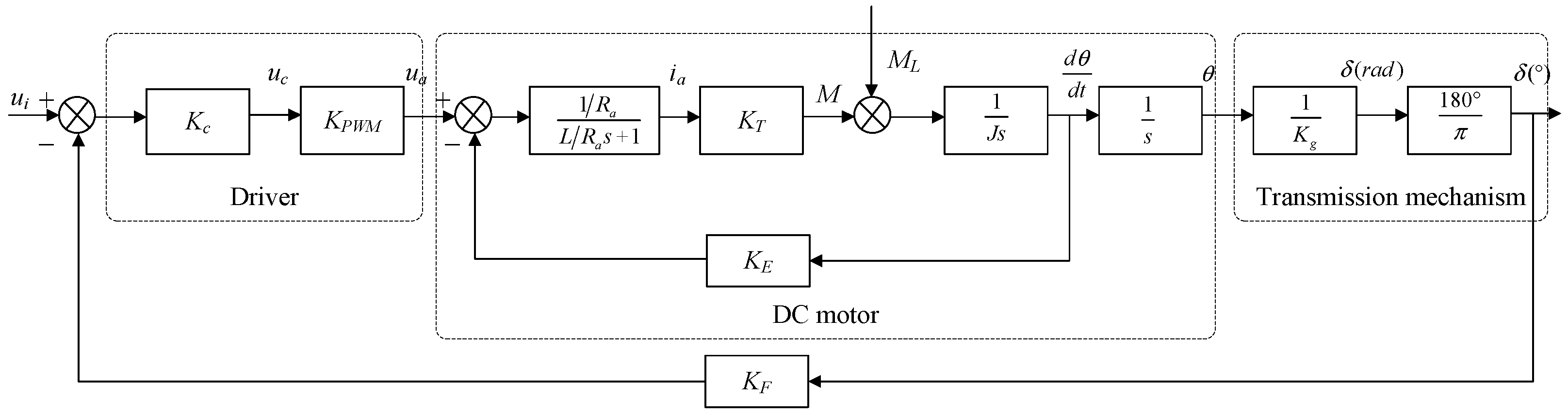
The drive system of the electric steering gear is generally composed of a controller, drive, DC motor, reduction transmission mechanism, feedback potentiometer, and other modules [10].

The DC motor is the core component of the electric steering gear. The mathematical model of its dynamic process can be established without considering the damping torque and friction torque. The voltage balance equation of the DC motor loop can be expressed as:

$$u_a=L\frac{d{i}_a}{dt}+i_a{R}_a+E_b$$

(1)

In the above formula, u_a is the motor loop voltage, i_a is the motor loop current, R_a is the motor circuit total resistance, E_b is the motor back electromotive force, and L is the total motor inductance.

The back electromotive force of a DC motor can be expressed as:

$$E_b=K_E\frac{d\theta }{dt}$$

(2)

In the above formula, K_E is back EMF (Electromotive Force) coefficient, θis DC motor rotation angle.

The torque equation and torque balance equation of a DC motor can be expressed as:

$$\begin{array}{l}M=K_T\times i_a\\ M=J\frac{d^2\theta }{d{t}^2}+M_L\end{array}\}$$

(3)

In the above formula, K_T is the torque coefficient, M is the motor torque, M_L is the load torque on the output shaft of the motor, and J is the total moment of inertia of the motor shaft.

Under no-load conditions (M_L = 0), the transfer function of a DC motor can be expressed as:

$$\frac{\theta (s)}{u_a(s)}=\frac{K_T}{s(JL{s}^2+J{R}_{a}s+K_T{K}_E)}$$

(4)

Suppose δ₀ is the output angle of the electric steering gear, and K_g is the transmission ratio of the transmission mechanism:

$${\delta }_0(s)=\frac{\theta (s)}{K_g}$$

(5)

The transfer function between the output angle of the electric steering gear and the input voltage [11] can be obtained from Equations (4) and (5), as follows:

$$\frac{{\delta }_0(s)}{u_a(s)}=\frac{K_T}{K_{g}s(JL{s}^2+J{R}_{a}s+K_T{K}_E)}$$

(6)

Let T_e = L/R_a, T_m = JR_a/K_EK_T, T_e is the electromagnetic time constant, T_m is the electromechanical time constant, then Equation (6) can be simplified to Equation (7):

$$\frac{{\delta }_0(s)}{u_a(s)}=\frac{\frac{1}{K_E{K}_g}}{s(T_e{T}_m{s}^2+T_{m}s+1)}$$

(7)

In the linear region, the transfer function of the PWM (Pulse Width Modulation) driver can be expressed as:

$$K_{PWM}=\frac{u_a(s)}{u_c(s)}$$

(8)

According to the principle of the feedback potentiometer, the transfer function of the feedback potentiometer is usually a constant, which can be expressed as:

$$K_F=\frac{u_f(s)}{\delta (s)}$$

(9)

In the above formula, K_F is the rudder surface feedback coefficient, δ is the output steering angle of the electric steering gear, and u_f is the feedback voltage feedback.

In summary, analyzing the composition and principle of each component of the electric steering gear, the linear transfer function block diagram of the electric steering gear drive system can be obtained, as shown in Figure 1.

The closed-loop transfer function of the electric steering gear drive system gained from Figure 1 is:

$$\frac{\delta (s)}{u_i(s)}=\frac{180K_c{K}_{PWM}/K_E{K}_g\pi }{s(T_e{T}_m{s}^2+T_{m}s+1)+180K_c{K}_{PWM}{K}_F/K_E{K}_g\pi }$$

(10)

Let K₁ = K_cK_PWM, K₂ = 180/K_EK_gπ, then Equation (10) can be simplified to Equation (11):

$$\frac{\delta (s)}{u_i(s)}=\frac{K_1{K}_2}{s(T_e{T}_m{s}^2+T_{m}s+1)+K_1{K}_2{K}_F}$$

(11)

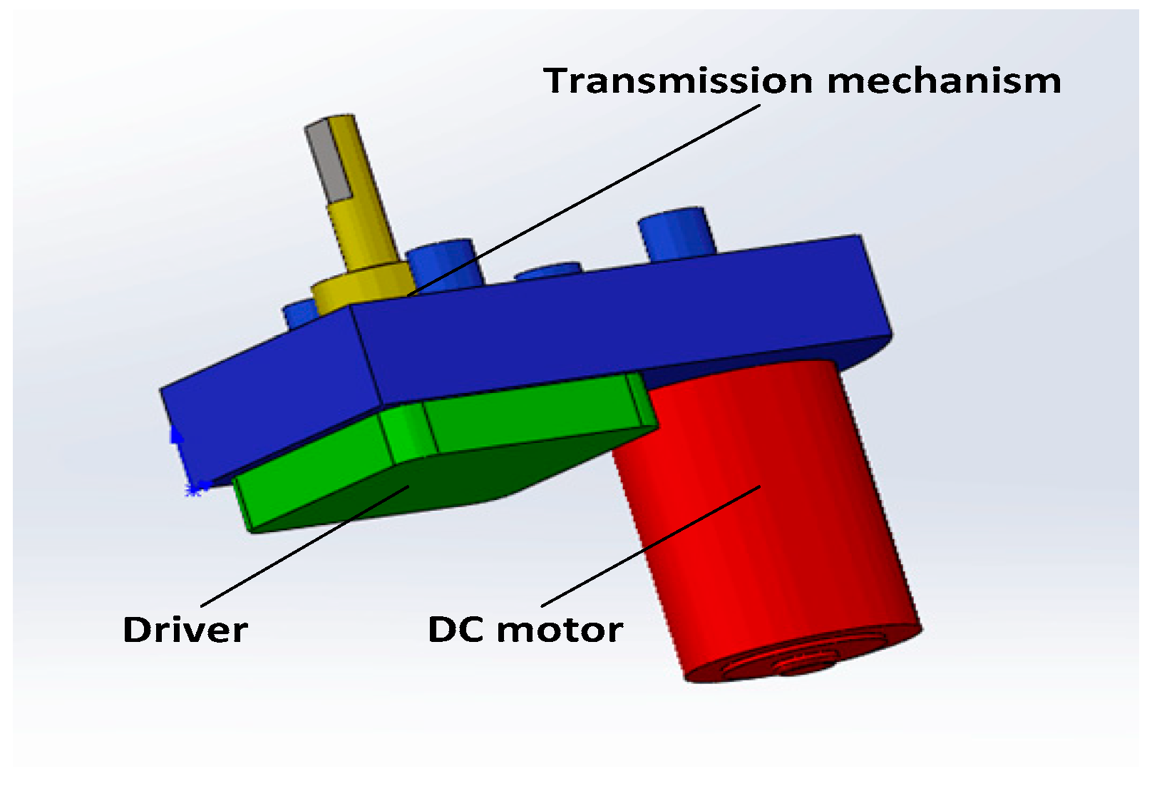
In this paper, the ASMC-03B electric steering gear which has stable power and with a speed reducer function is used at each joint, as shown in Figure 2.

The technical parameters of ASMC-03B electric steering gear are shown in

Table 1. Main parameters of the ASMC-03B electric steering gear.

Main Parameters	Value
Electromagnetic time constant (Te/s)	0.0006
Electromechanical time constant (Tm/s)	0.008
Rudder surface feedback coefficient (KF)	1
Transmission ratio of the transmission mechanism (Kg)	4:1
DC motor back EMF coefficient (KE)	1.8
Signal drive gain (K1)	45

.

Substituting all the parameters of Table 1 into Equation (11), the closed-loop transfer function of the electric steering gear can be obtained as follows:

$$G_B(s)=\frac{\delta (s)}{u_i(s)}=\frac{360}{4.8\times {10}^{-6}{s}^3+8\times {10}^{-3}{s}^2+s+360}$$

(12)

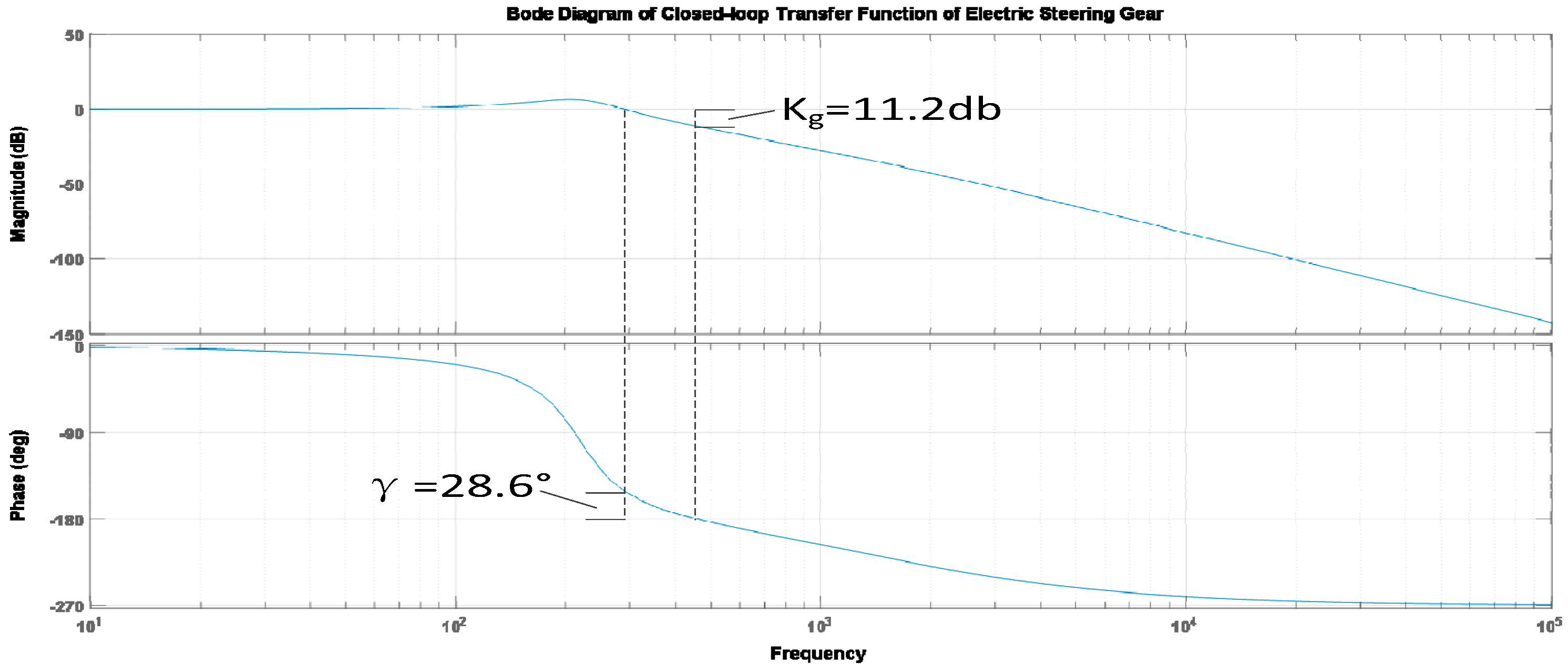
By analyzing the amplitude–frequency characteristics of the closed-loop transfer function in Simulink’s linear analysis tool, the Bode diagram of the closed-loop transfer function can be obtained, as shown in Figure 3.

In engineering practice, in order to ensure the system has a satisfactory stability reserve, it is generally desirable to have a phase margin in the range of 30 to 60 and an amplitude margin more than 6 dB [12].

The Bode diagram of the closed-loop transfer function has a phase margin value of 28.6 and an amplitude margin value of 11.2 dB, meaning the closed-loop system is stable.

3. System Design and Simulation Analysis

3.1. Steering Gear Drive Control System

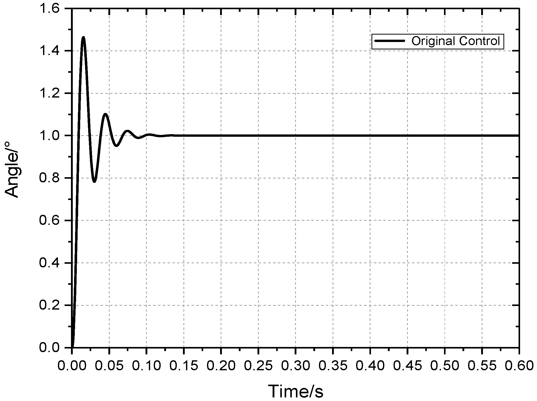
The closed-loop transfer function of the established electric steering gear is packaged into a submodule, and the unit step signal is used as an input signal for response testing, which is called the original control. The simulation results of the original control are shown in Figure 4 and the simulation results are shown in

Table 2. Simulation results of original control.

Control Method	Rise Time (tr/s)	Adjust Time (ts/s)	Overshoot (M/%)
Original control	0.0078	0.0504	46.41

.

Because the electric servo is equipped with a potential feedback device, its interior is a semiclosed-loop system. When the original control is performed, the system can be stabilized after a short adjustment. At the same time, ensuring the accuracy of the system adjustment, the rise time and adjustment time are shorter. However, it has a very large overshoot, the oscillation is strong, and the system is unstable. Therefore, it is necessary to combine control methods to reduce the overshoot and oscillation of the system.

3.2. PID Control System

PID control is a typical negative feedback control method. The input value of the system is subtracted from the output value of the system to obtain the deviation of the system’s output, and then proportional, integral, and derivative control of the output deviation is performed [13].

In the continuous time domain, the PID control algorithm can be expressed as:

$$u(t)=K_p[e(t)+\frac{1}{T_i}{\displaystyle {\int }_0^{t}e(t)dt+T_d\frac{de(t)}{dt}}]$$

(13)

In the above formula, K_p is the proportion coefficient, T_i is the integral time constant, and T_d is the differential time constant.

Because the steering gear drive system has a very large overshoot, this article aims to reduce the overshoot of the system. According to the PID parameter setting principle [14]: the function of the proportional coefficient K_p is to speed up the response speed of the system and improve the adjustment accuracy of the system, the integral time constant T_i is to eliminate the steady-state error of the system. The function of the differential time constant T_d is to improve the dynamic performance of the system.

The discrete form of the PID formula can be further derived from Equation (13) as follows:

$$u(k)=K_{p}e(k)+K_i{\displaystyle \sum _{j=0}^{k}e(j)+}{K}_d[e(k)-e(k-1)]$$

(14)

In the above formula, K_p is the proportion coefficient, K_i is the integral coefficient, and K_d is the differential coefficient.

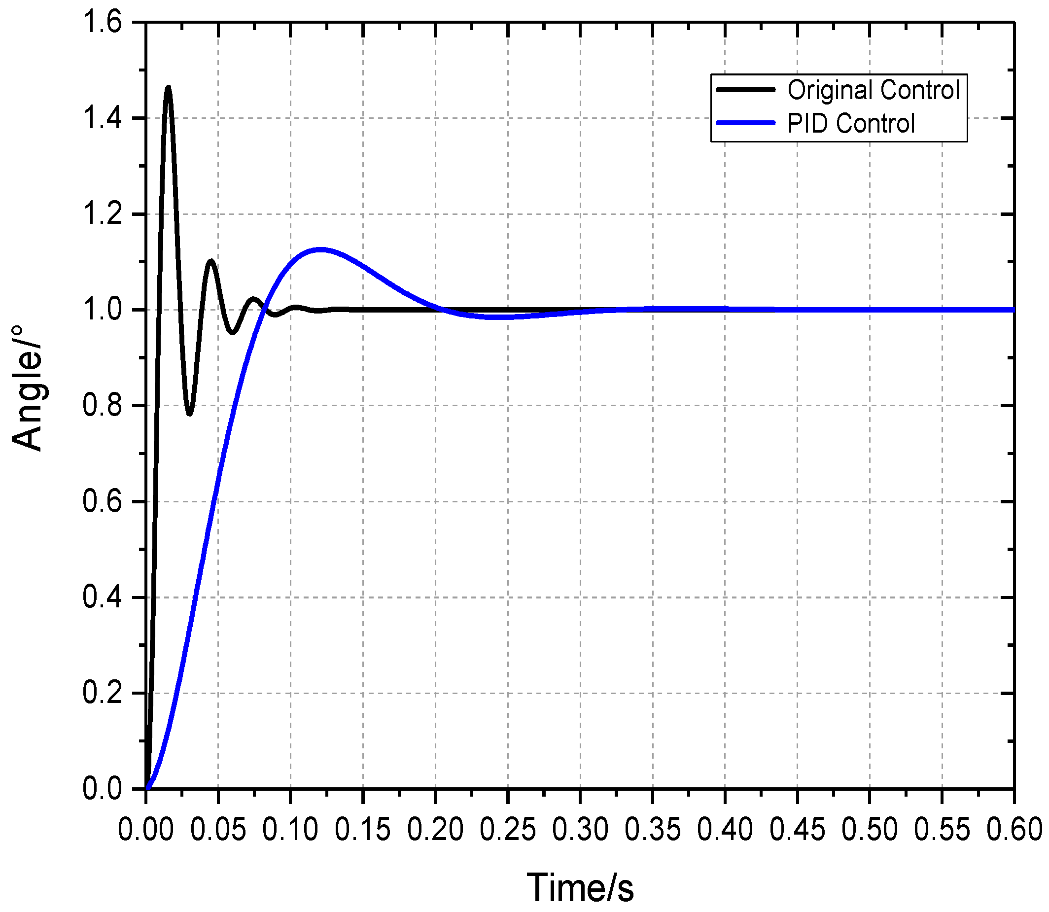
It is finally determined that when K_p is within the range of [0.1, 1], K_i is within the range of [10, 30], and K_d is within the range of [0.01, 0.03], the system overshoot is less than 15%. When K_p = 0.1, K_i = 30, and K_d = 0.03, PID control of the system uses the unit step signal as the input signal of the model. The simulation result of PID control is shown in Figure 5, and the simulation data of PID control are shown in

Table 3. PID control simulation data.

Control Method	Rise Time (tr/s)	Adjust Time (ts/s)	Overshoot (M/%)
Original control	0.0078	0.0504	46.41
PID control	0.0573	0.172	12.56

.

After the preliminary adjustment of PID control, the simulation results show that the system became more stable, accurately reached the predetermined position, and ensured the accuracy of the adjustment by using the original control and PID control. The rise time and the adjustment time of PID control increased slightly, but the overshoot was reduced by 34.25%. The simulation results show that the application of traditional PID control technology increases the rise time and adjustment time of the joint movement but greatly reduces the overshoot and enhances the stability of motion.

3.3. Fuzzy PID Control System

For control objects with large hysteresis, large inertia, and complex signal tracking, PID control is also very limited, but the fuzzy PID control technology can be used to improve PID control defects [15].

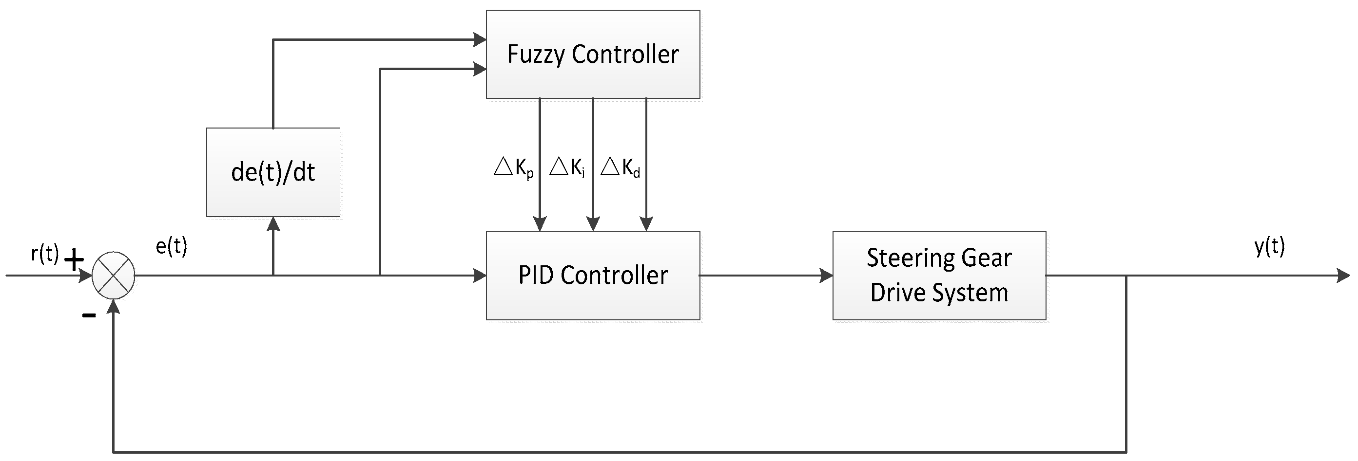
The fuzzy PID controller is implemented on the basis of the conventional PID controller. Generally, e(t) and de(t)/dt are used as the input quantity of fuzzy control, and the ΔK_p, ΔK_i and ΔK_d are used as the output quantity of fuzzy control. It is a fuzzy controller with two-input and three-output [16], as shown in Figure 6.

The new PID control parameters can be formed by adding the fuzzy parameters in the regular PID parameters:

$$\begin{array}{r}{K_p}^{\prime }=K_p+\Delta K_p\\ {K_i}^{\prime }=K_i+\Delta K_i\\ {K_d}^{\prime }=K_d+\Delta K_d\end{array}\}$$

(15)

Use the PID parameters above, K_p = 0.1, K_i = 30, and K_d = 0.03. Add the value of ΔK_p, ΔK_i and ΔK_d of the fuzzy control output to calculate the new PID parameters.

Determine the basic domain of e(t) as [−1,1], the basic domain of de(t)/dt is [−0.014,0.014], the basic domain of ΔK_p is [−0.1,0.1], the basic domain of ΔK_i is [−20,20], and the basic domain of ΔK_d is [−0.02,0.02]. For convenient calculation, we set the fuzzy sets of input and output values as [−2, 2]. The quantization factor of e(t), de(t)/dt, ΔK_p, ΔK_i and ΔK_d respectively, is 2, 0.007, 0.05, 10, and 0.01. Using the e(t) and de(t)/dt as the fuzzy control input, the ΔK_p, ΔK_i and ΔK_d as the fuzzy control output, the fuzzy control of the two inputs and three outputs is performed.

According to actual experience, the values of ΔK_p, ΔK_i, and ΔK_d under different error and rate of error change need to meet the following adjustment principle [17]:

(1) When the error is large, improve the system’s fast-tracking performance. No matter how much the error varies, it should take a larger value of ΔK_p and a smaller value of ΔK_d. At the same time, in order to avoid a large overshoot, the integral link should be limited and take a smaller value of ΔK_i.

(2) When the error is at a medium size, in order to reduce the overshoot of the system response, the value of ΔK_p should be smaller. In order to ensure the response speed of the system, the value of ΔK_i and ΔK_d should be moderate. The value of ΔK_d has a greater impact on the system response.

(3) When the error is small, in order to ensure the system has good steady-state performance, the value of ΔK_p and ΔK_i should be larger. At the same time, in order to avoid the oscillation of the system near the set value and consider the anti-interference performance of the system, the value of ΔK_d can be larger when the rate of error change is small, the value of ΔK_d should be smaller when the rate of error change is larger.

Based on experience, the fuzzy control rule table shown in

Table 4. Fuzzy rule table of three parameters.

ΔKp fuzzy rule table
	de(t)/dt	NL	NS	ZO	PS	PL
e(t)
NL		PL	PS	PS	ZO	ZO
NS		PS	PS	ZO	ZO	ZO
ZO		PS	ZO	ZO	ZO	NS
PS		ZO	ZO	ZO	NS	NS
PL		ZO	ZO	NS	NS	NL
ΔKi fuzzy rule table
	de(t)/dt	NL	NS	ZO	PS	PL
e(t)
NL		NL	NL	NS	NS	ZO
NS		NS	NS	NS	ZO	PS
ZO		NS	NS	ZO	PS	PS
PS		NS	ZO	PS	PS	PS
PL		ZO	PS	PS	PL	PL
ΔKd fuzzy rule table
	de(t)/dt	NL	NS	ZO	PS	PL
e(t)
NL		NS	NL	NL	NL	NS
NS		NS	NL	NL	NS	NS
ZO		NS	NS	NS	NS	NS
PS		ZO	ZO	ZO	ZO	ZO
PL		PS	PS	PS	PS	PS

was produced through the simulation experiment.

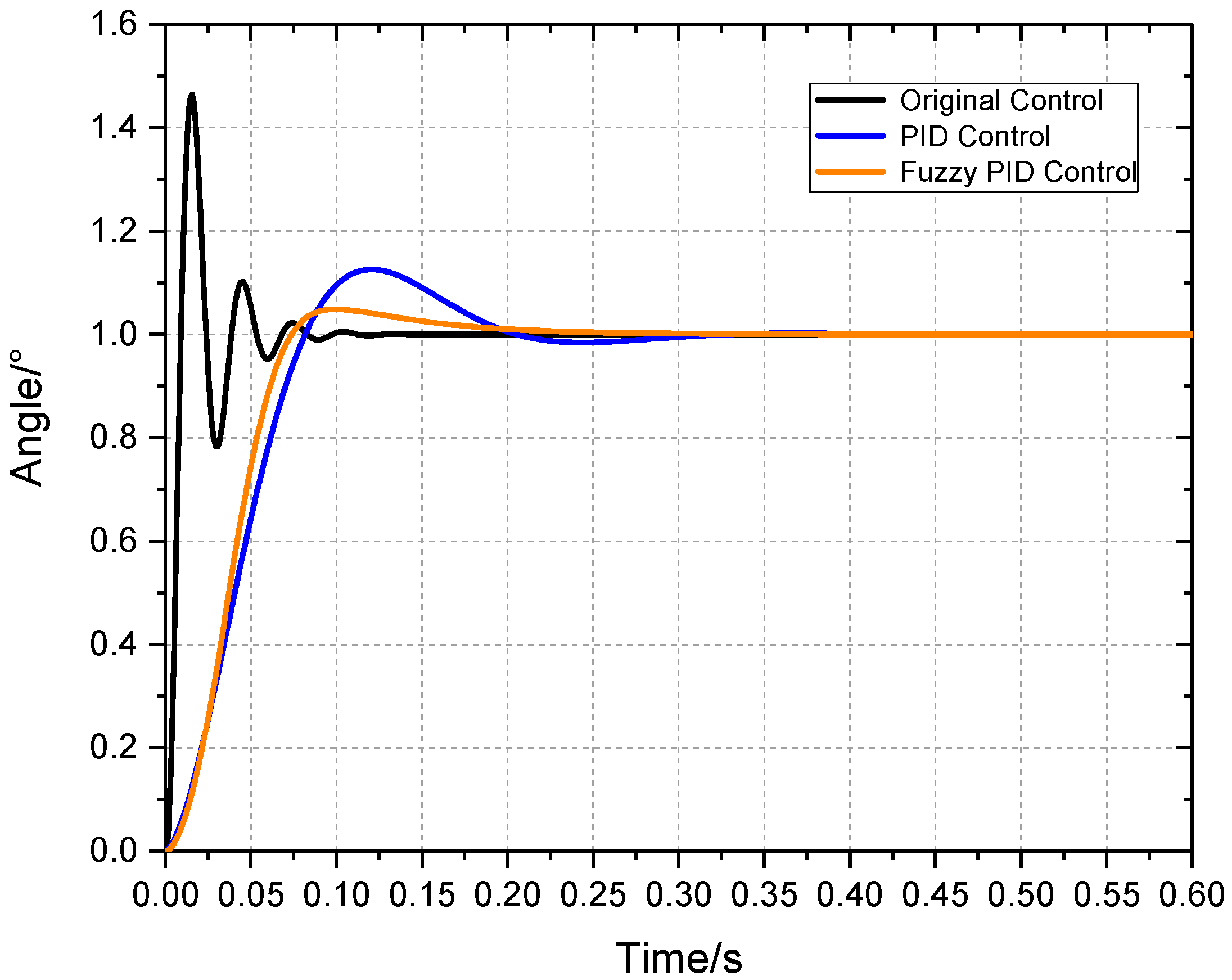
The simulation is performed according to the fuzzy rules of

Table 5. Fuzzy PID control simulation data.

Control Method	Rise Time (tr/s)	Adjust Time (ts/s)	Overshoot (M/%)
Original control	0.0078	0.0504	46.41
PID Control	0.0573	0.172	12.56
Fuzzy PID Control	0.0468	0.0991	4.86

. The simulation result of the fuzzy PID control is shown in Figure 7.

The simulation results show that compared with the PID control, the rise time and the adjustment time of the fuzzy PID control are further reduced based on the original advantages, and the overshoot is reduced by 7.70%, which enhances the rapidity and stability of the system adjustment.

3.4. Orthogonal-Fuzzy PID Control System

Due to the randomness of the PID parameters selected by experience, the control effect of the fuzzy PID cannot be optimal. In this paper, the orthogonal optimization method is adopted for the setting of PID parameters. The orthogonal optimization method can quickly and accurately select a set of optimal PID parameters. Therefore, the performance of the system can be further improved by the fuzzy control of the PID parameters obtained by orthogonal optimization [18].

3.4.1. Traditional Orthogonal Test Procedure

(1) Define the purpose of the test and determining the indicator.

The purpose of the test is to select a suitable set of PID parameters to optimize the accuracy and stability of the manipulator control system. The most important indicator in the control system is overshoot and adjustment time. However, the preliminary adjustment of the PID parameters can greatly reduce the overshoot of the system when performing traditional PID control in this paper, so only the adjustment time is determined as an indicator of the test.

(2) Determine the factors and levels, and formulate the factor level table.

Obviously, this experiment is to study the influence of three PID parameters on the control index, so the three parameters determined are K_p, K_i and K_d. The selection of the horizontal range of the orthogonal table is closely related to the theoretical level and practical experience of the operators. The selection of the horizontal range is based on a large amount of practical experience in this paper [19].

(3) Select the orthogonal table for head design and determine the test plan.

When an orthogonal table is selected, the smallest orthogonal table that satisfies the factors and levels can be selected according to the number of levels and factors. In order to ensure the reliability of the test, this paper selects the orthogonal table L₉(3⁴) (four factors and three levels). Single-factor experiments show that although there are interactions among the three parameters, the significance of the impact is relatively small, so the interaction is not considered [20].

(4) Analysis and comparison of test data.

This test uses visual analysis to analyze data.

(5) Verification of test results.

Substitute the analyzed optimal data into the system to see if it improves the system’s overshoot and adjustment time.

3.4.2. PID Control and Simulation Based on Orthogonal Experiments

After the initial PID adjustment, the system can meet the work demand when the overshoot is less than 15%. Next, aiming at reducing the adjustment time of the system, orthogonal testing was performed to set the PID parameters. An orthogonal table of four factors and three levels was designed. The factor level table is shown in

Table 6. Factor level table.

Level	Kp	Ki	Kd
1	0.1	10	0.01
2	0.5	20	0.02
3	1	30	0.03

.

According to the factor level table, the simulation is carried out sequentially with the goal of adjustment time improvement, and the simulation data are shown in

Table 7. Data table of PID orthogonal experimental results.

Test Number	Kp	Ki	Kd	Empty column	Adjust Time (s)
1	1	1	1	1	0.3926
2	1	2	2	2	0.1261
3	1	3	3	3	0.0673
4	2	1	3	3	0.4064
5	2	2	1	1	0.1967
6	2	3	2	2	0.0877
7	3	1	2	2	0.4732
8	3	2	3	3	0.1946
9	3	3	1	1	0.1435
1-level experiment mean	0.1953	0.4240	0.2443
2-level experiment mean	0.2303	0.1725	0.2290
3-level experiment mean	0.2704	0.0995	0.2328
range	0.0751	0.3245	0.0115

.

As can be seen from Table 7, the range of three parameters K_p, K_i and K_d are R_Kp = 0.0751, R_Ki = 0.3245, and R_Kd = 0.115, respectively. These values satisfy the relationship R_Ki > R_Kp > R_Kd. It shows that K_i is the factor that has the greatest impact on the settling time, followed by K_p, and finally K_d. Combined with horizontal experiments of the mean value analysis of each factor, the effect of PID control is better when K_p = 0.1, K_i = 30, and K_d = 0.02.

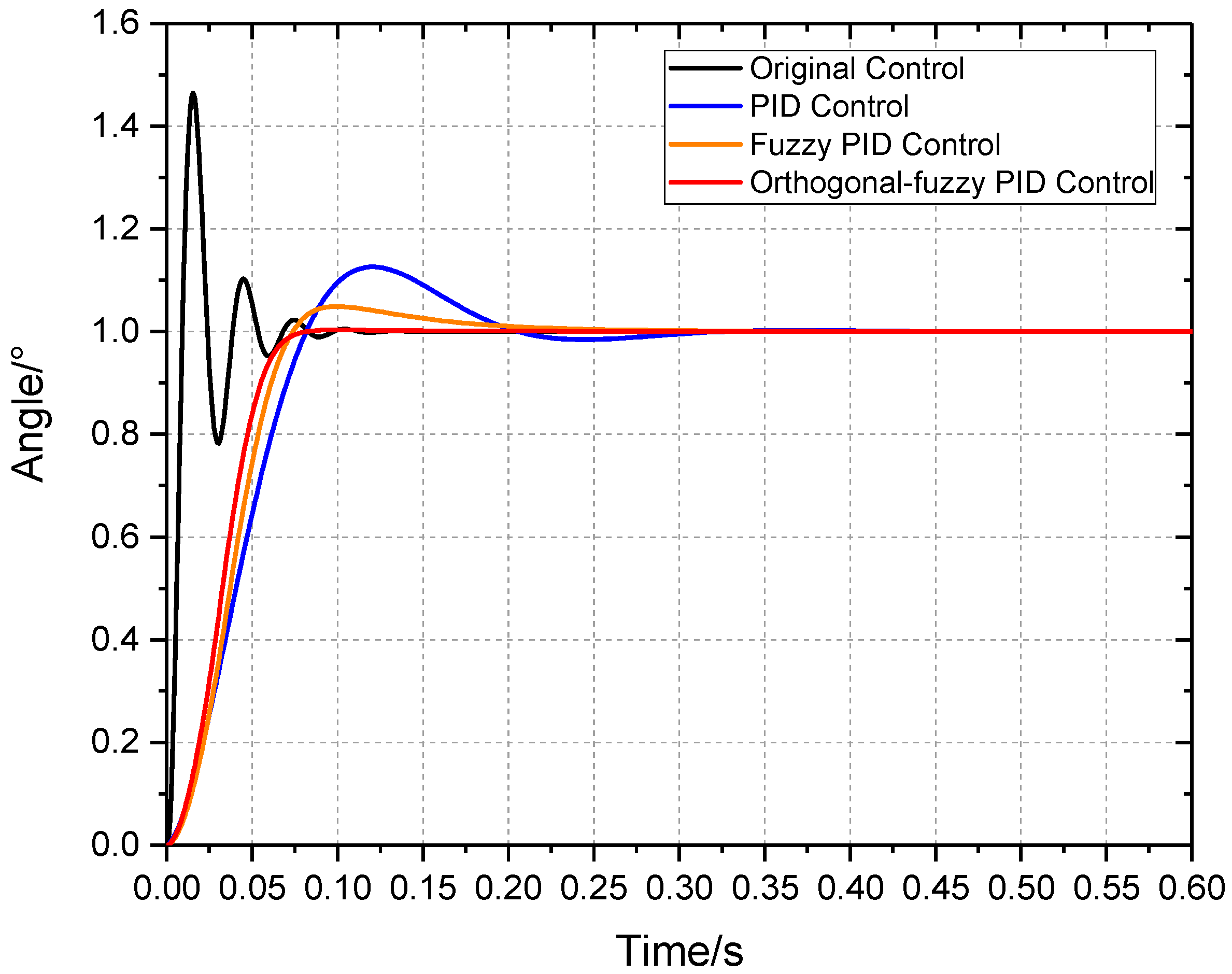
The simulation results of the orthogonal-fuzzy PID control are shown in Figure 8, and the simulation data of the orthogonal-fuzzy PID control are shown in

Table 8. Orthogonal-Fuzzy PID control simulation data.

Control Method	Rise Time (tr/s)	Adjust Time (ts/s)	Overshoot (M/%)
Original control	0.0078	0.0504	46.41
PID Control	0.0573	0.172	12.56
Fuzzy PID Control	0.0468	0.0991	4.86
Orthogonal-Fuzzy PID Control	0.0426	0.0615	0.26

.

The simulation results show that the system can be stabilized by separately using original control, PID control, fuzzy PID control, and orthogonal-fuzzy PID control. Compared with the original control, the rise time and adjustment time of the PID control increase slightly, but the overshoot is significantly reduced, which can enhance system’s motion control stability. Compared with the PID control, the rise time, adjustment time, and overshoot of the fuzzy PID control are reduced. The adjustment speed is accelerated while enhancing the stability of the system. Compared with fuzzy PID control, the system of orthogonal-fuzzy PID control with the factor level combination (K_p = 0.1, K_i = 30 and K_d = 0.02) is optimal, and the rise time and the adjustment time are reduced. The oscillation process of the system near the steady state is reduced and the stability of the system control is enhanced. According to the above simulation results, the orthogonal-fuzzy PID control combines the advantages of fuzzy control and orthogonal optimization, which can realize the real-time setting and control of PID parameters, and has good regulation performance for the joint drive of the manipulator.

4. Experiment and Analysis

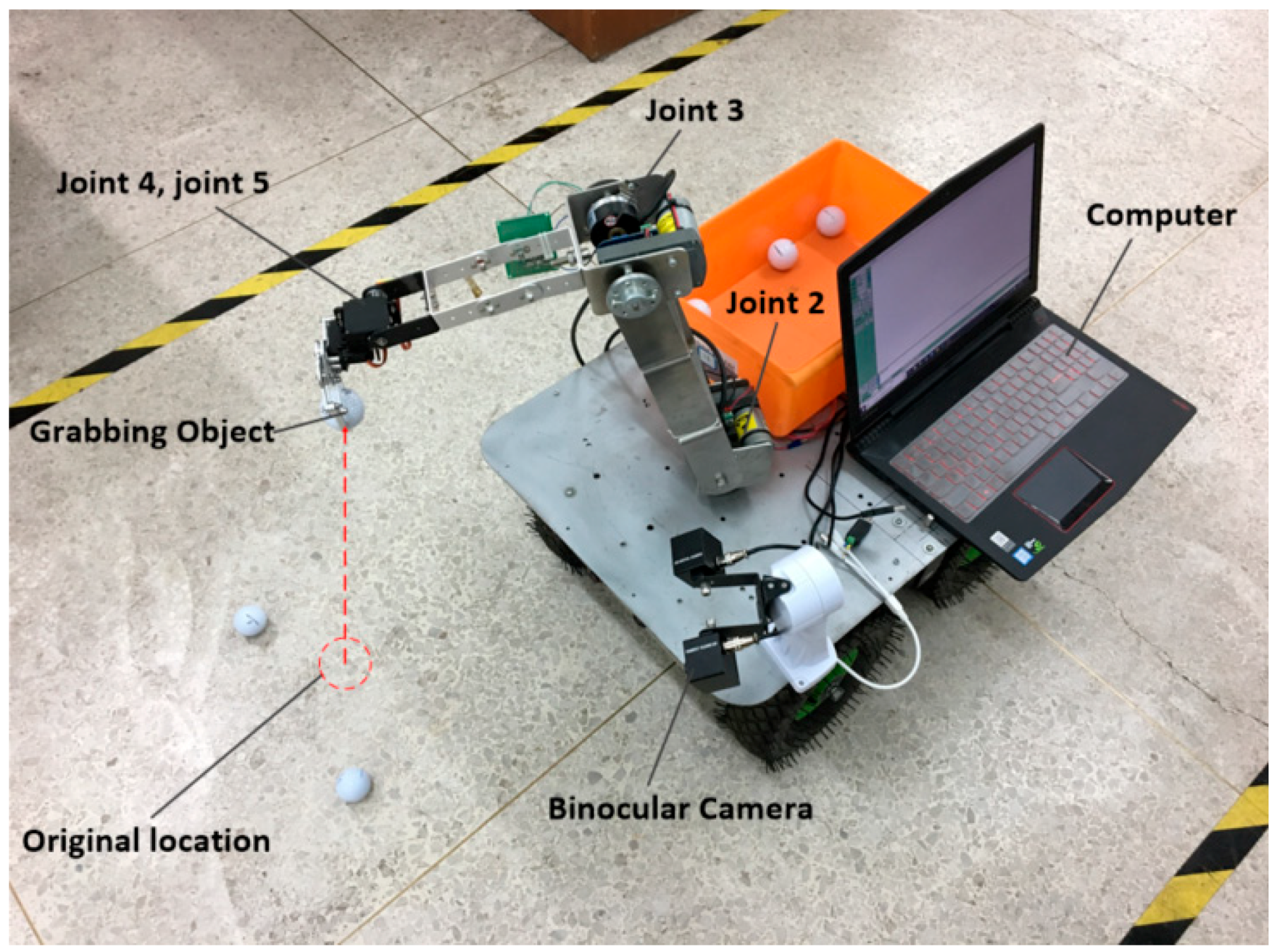
The experimental platform is shown in Figure 9. Joint 3 is equipped with the HK50-D8G type encoder. The experiment uses the STM32 embedded system for fuzzy PID calculation and robot control and uses a serial port for data communication and feedback. The robotic arm of the platform shown in Figure 9 has a total length of about 560 mm.

4.1. Joint Drive System

When the angle error of the manipulator is measured by the single-joint drive system, the other joints are locked and a single joint rotates at different angles θ₂. Original control, PID control, and fuzzy PID control are used in the joint drive system and the actual rotation angle of the manipulator joint is measured by the encoder. Experiments were carried out at angles of 30, 60, and 75, and the joint angle error and average adjustment time of the manipulator were obtained. The measurement results are shown in

Table 9. Angular error and average adjustment time of the manipulator joint.

Input Angle (θ2/°)	Control Method	Average Angular Error (°)	Angle error Maximum (°)	Average Angular Relative Error	Average Adjustment Time (s)
30°	Original control	−3.224	−3.75	10.746%	2.18
	Fuzzy PID Control	2.27	2.93	7.55%	3.56
	Orthogonal-Fuzzy PID Control	1.95	2.23	6.5%	3.24
60°	Original control	−4.585	−4.69	7.642%	3.28
	Fuzzy PID Control	−2.061.	−3.75	3.44%	4.40
	Orthogonal-Fuzzy PID Control	−1.642	−0.94	2.737%	4.03
75°	Original control	8.208	8.28	9.657%	3.30
	Fuzzy PID Control	5.015	5.79	5.97%	5.97
	Orthogonal-Fuzzy PID Control	2.655	2.78	3.124%	5.31

.

From the analysis of the measurement results, it can be concluded that:

Compared with the original control, the adjustment time of fuzzy PID control and orthogonal-fuzzy PID control increase by 1.2 s. Compared with fuzzy PID control, the adjustment time and rise time of the orthogonal-fuzzy PID control decreased slightly, but the oscillation process near the steady state was reduced and the stability of the system was enhanced. Compared with the original control, the average stable angular error of the fuzzy PID control and the orthogonal-fuzzy PID control were reduced to different degrees, and the average stable angular relative error was reduced by about 4.5%. It shows that the two control methods play a role in feedback regulation. Compared with the fuzzy PID control, the average stable angular error of orthogonal-fuzzy PID control was reduced by a small amount, and the average stable angular relative error was reduced by about 1.5%.

These results show that the inaccuracy of the PID parameters selected by experience result in the fuzzy control not being optimal. However, the orthogonal-fuzzy PID control can further reduce the angle control error and increase the accuracy of system adjustment. The robot still has certain errors with original control, fuzzy PID control, and orthogonal-fuzzy PID control. The reason may be the influence of the torque generated by the robot’s own weight and the influence of assembly error and measurement error during the measurement.

4.2. Manipulator Drive Systems

When the manipulator drive system measures the positioning error, the position coordinates of the end of the manipulator are given and the controller performs original control, fuzzy PID control, or orthogonal-fuzzy PID control to reach the target position, and calculates the coordinate error of the theoretical position and the actual position.

The coordinates of X and Z are given when the position coordinates of the end of the manipulator are on the Y axis (Y = 0), that is, five groups of joint angles of θ₂ and θ₃ are given, which are (15,15), (30,30), (45,45), (60,60), (75,75), respectively. After three experimental tests, the position error of the manipulator can be measured to get the average position error of each coordinate. The measurement results are shown in

Table 10. Positioning error of the two-degrees-of-freedom manipulator.

Theoretical Coordinate (mm)	Angle of Two Joints (θ2, θ3/°)	Control Method	Actual Coordinate (mm)	Average Position Error of Multiple Measurements (mm)
(548.75, 0, 85.41)	15, 15	Original control	(550.06, 0, 85.35)	2.20
		Fuzzy PID Control	(549.94, 0, 85.37)	1.19
		Orthogonal-Fuzzy PID Control	(549.59, 0, 85.90)	0.97
(515.79, 0, 165.00)	30, 30	Original control	(519.97, 0, 164.86)	5.11
		Fuzzy PID Control	(518.63, 0, 167.72)	3.93
		Orthogonal-Fuzzy PID Control	(513.06, 0, 167.29)	3.84
(463.35, 0, 233.35)	45, 45	Original control	(449.85, 0, 257.17)	15.91
		Fuzzy PID Control	(460.48, 0, 236.18)	4.03
		Orthogonal-Fuzzy PID Control	(463.64, 0, 234.79)	1.49
(395.00, 0, 285.79)	60, 60	Original control	(385.53, 0, 296.20)	17.43
		Fuzzy PID Control	(393.81, 0, 289.97)	4.18
		Orthogonal-Fuzzy PID Control	(397.92, 0, 286.44)	3.02
(315.41, 0, 318.76)	75, 75	Original control	(291.51, 0, 344.25)	18.81
		Fuzzy PID Control	(304.38, 0, 323.65)	12.07
		Orthogonal-Fuzzy PID Control	(310.20, 0, 316.37)	6.15

.

From Table 10, it can be concluded that compared with the original control, the fuzzy PID control reduces the average position error by about 50%. Compared with the fuzzy PID control, the orthogonal-fuzzy PID control reduces the average position error by about 30%. It shows that the uncertainty of the PID parameters selected by experience causes adjustment error of the fuzzy control system. In the experiment, the system of orthogonal-fuzzy PID control is stable and the manipulator does not oscillate near the steady state. Orthogonal-fuzzy PID control further reduces the system error and enhances the accuracy of the system. When the rotation angle of the joint is small, the mechanical error is small, so the error of original control is smaller. At the same time, fuzzy PID control and orthogonal-fuzzy PID control have less adjusting force but are more precise. When the rotation angle of the joint is large, the mechanical error suddenly increases due to the force problem.

4.3. Comparative Analysis

The simulation analysis of fuzzy PID control and orthogonal fuzzy PID control shows that the response curve enters the error range of 5% of the steady state value at the beginning. Therefore, the maximum value of the steady-state error of the fuzzy PID control system is 4.86%, and the maximum value of the steady-state error of the orthogonal fuzzy PID system is 0.26%. The angles of two joints θ₂, θ₃ are 15, 45, and 75, and the data and error of the robot’s simulated coordinates are compared with the coordinates of the actual robot in

Table 11. Comparison of simulation and experimental results.

Control Method	Angle of Two Joints (θ2, θ3/°)	Theoretical Coordinate (mm)	Simulation Coordinates (mm)	Experimental Coordinate (mm)	Simulation Error (mm)	Experimental Error (mm)
Fuzzy PID Control	15, 15	(548.75, 0, 85.41)	(547.70,0,89.24)	(549.94, 0, 85.37)	3.99	1.19
	45, 45	(463.35, 0, 233.35)	(454.76,0,241.62)	(460.48, 0, 236.18)	8.75	4.03
	75, 75	(315.41, 0, 318.76)	(296.07,0,323.54)	(304.38, 0, 323.65)	19.90	12.07
Orthogonal fuzzy PID Control	15, 15	(548.75, 0, 85.41)	(548.60,0,85.63)	(549.59, 0, 85.90)	0.27	0.97
	45, 45	(463.35, 0, 233.35)	(462.87,0,233.82)	(463.64, 0, 234.79)	0.70	1.49
	75, 75	(315.41, 0, 318.76)	(314.32,0,319.04)	(310.20, 0, 316.37)	1.13	6.15

.

From the analysis of Table 11, the errors of the fuzzy PID and the orthogonal fuzzy PID control systems increase as the angle of the manipulator increases, and the simulated coordinates are consistent with the experimental coordinates. Since the maximum error of the fuzzy PID control system near the steady state of 5% is much larger than the error of the orthogonal fuzzy PID control, the simulation error is large.

However, compared with the fuzzy PID control system, the simulation error and experimental error of the orthogonal fuzzy PID control system are significantly reduced, which indicates that the orthogonal optimization greatly improves the fuzzy PID control effect.

5. Conclusions

(1) Compared with the fuzzy PID control method, the adjustment time, rise time, and overshoot of the orthogonal fuzzy PID control are reduced to a certain extent. At the same time, the maximum value of 0.26% of the orthogonal fuzzy-PID control system is far less than 4.86% of the fuzzy-PID control system when it has just entered the steady state value of 5%, which reduces the oscillation near the steady state. The experimental process also revealed that the oscillation of the manipulator near the steady state was significantly reduced, thus the orthogonal fuzzy PID control can improve the stability of the system’s motion control.

(2) Compared with the original control, the adjustment time of the fuzzy PID control is increased by 1.2 s, and the relative error of the average angle is reduced by about 4.5%. However, the system using orthogonal-fuzzy PID control has a slight decrease in adjustment time and rise time, and the relative error of the average angle is reduced by about 1.5% and the average position error is reduced by about 30%. The results show that orthogonal fuzzy PID control can further improve the accuracy of the system.

(3) Due to the randomness of the empirically selected PID parameters, the control effect of the fuzzy PID is not optimal. Using the orthogonal test method to adjust the PID parameters can reduce the number of tests and quickly determine the appropriate PID parameters and thus improve the accuracy and stability of the fuzzy PID control system. At the same time, compared with the fuzzy PID control system, the simulation error and experimental error of the orthogonal fuzzy PID control system are significantly reduced, which indicates that the orthogonal optimization greatly improves the fuzzy PID control effect.

References

- Fengying, M. An improved fuzzy PID control algorithm applied in liquid mixing system. In Proceedings of the 2014 IEEE International Conference on Information and Automation (ICIA), Hailar, China, 28–30 July 2014. [Google Scholar]
- Engin, Y.; Tufan Kumbasar, M.; Dodurka, F. Peak observer based self-tuning of type-2 fuzzy PID controllers. In Proceedings of the International Conference on Artificial Intelligence Applications and Innovations (IFIP), Rhodes, Greece, 19–21 September 2014; pp. 487–497. [Google Scholar]
- Wang, Y.; Lu, Y. Design of longitudinal predictive re-entry guidance law based on variable universe fuzzy-PI composite control. J. Control Theory Appl. 2012, 2, 264–267. [Google Scholar] [CrossRef]
- Lee, K.; Im, D.Y.; Kwak, B.; Ryoo, Y.J. Design of Fuzzy-PID controller for path tracking of mobile robot with differential drive. Int. J. Fuzzy Logic Intel. Syst. 2018, 18, 220–228. [Google Scholar]
- Wang, T.Y.; Chang, C.D. Hybrid fuzzy PID controller design for a mobile robot. In Proceedings of the 2018 IEEE International Conference on Applied System Invention (ICASI), Chiba, Japan, 13–17 April 2018; pp. 650–653. [Google Scholar]
- Lu, J.; Wan, J.X.; Zhu, Z.D. Fuzzy PID control application in manipulator controller. Control Eng. Chin. 2009, 16, 155–157. [Google Scholar]
- Lingfeng, T.; Wang, Y. The PID control for electro-hydraulic servo system based on orthogonal test. In Proceedings of the International Forum on Computer Science—Technology and Applications (IFCSTA), Chongqing, China, 25–27 December 2009; Volume 3, pp. 255–258. [Google Scholar]
- Peng, A.H.; Sun, X.D.; Wang, Z.M. Parameter turning for PID controllers based on orthogonal experiment. Mech. Sci. Technol. Aerosp. Eng. 2011, 30, 1028–1032. [Google Scholar]
- Rohan, R.; Bambulkar Gargi, S.; Phadke, S.S. Movement control of robot using fuzzy PID algorithm. In Proceedings of the 3rd International Conference on Electrical, Electronics, Engineering Trends, Communication, Optimization and Sciences, Tadepalligudem, India, 1–2 June 2016. [Google Scholar]
- Zhang, W.; Wang, J.; Hou, W. New method of DC motor selection for the design of electric steering gear. Proc. Autom. Instrum. 2016, 17, 95–98. [Google Scholar]
- WenFu, Q. The Design & Implementation of Actuator Based DSP; Tsinghua University: Beijing, China, 2004. [Google Scholar]
- ZhaoYan, X.; HongJun, Z.; XiuPing, Y. Mechanical Control Engineering Foundation; Electronic Industry Press: Beijing, China, 2011; Volume 1, pp. 165–168. [Google Scholar]
- Madhushani, T.W.U.; Maithripala, D.H.S.; Berg, J.M. Feedback regularization and geometric PID control for trajectory tracking of mechanical systems: Hoop robots on an inclined plane. In Proceedings of the American Control Conference, Seattle, WA, USA, 24–26 May 2017; pp. 3938–3943. [Google Scholar]
- Kuantama, E.; Vesselenyi, T.; Dzitac, S. PID and Fuzzy-PID control model for quadcopter attitude with disturbance parameter. Int. J. Comput. Commun. Control 2017, 12, 519–532. [Google Scholar] [CrossRef]
- Chao, C.-T.; Sutarna, N.; Chiou, J.-S.; Wang, C.-J. An Optimal Fuzzy PID Controller Design Based on Conventional PID Control and Nonlinear Factors. Appl. Sci. 2019, 9, 1224. [Google Scholar] [CrossRef]
- Li, D.; Fu, Y.; Yang, L. Coupling dynamic modeling and simulation of three-degree-of-freedom micro-manipulator based on piezoelectric ceramic of fuzzy PID. Mod. Phys. Lett. B 2017, 31, 24. [Google Scholar]
- Dou, Y.; Qian, L.; Feng, J. Design and simulation of fuzzy PID control system based on matlab. Electr. Sci. Technol. 2015, 28, 119–122. [Google Scholar]
- Zhang, Z.K.; He, L. Based on orthogonal experiment method PID simulation control of pumping unit. Appl. Mech. Mater. 2013, 40, 580–585. [Google Scholar] [CrossRef]
- Noshadi, A.; Shi, J.; Lee, W.S. Optimal PID-Type fuzzy logic controller for a multi-input multi-output active magnetic bearing system. Neural Comput. Appl. 2016, 27, 2031–2046. [Google Scholar] [CrossRef]
- Lin, J.L.; Lin, C.L. The use of the orthogonal arry with grey relational analysis to optimize EDM process with multiple performance characteristics. Int. J. Mach. Tools Manuf. 2002, 42, 237–244. [Google Scholar] [CrossRef]
Figure 1.
Transfer function block diagram of the electric steering gear drive system.
Figure 2.
ASMC-03B electric steering gear.
Figure 3.
Bode diagram of the closed-loop transfer function of the steering gear.
Figure 4.
Original control Simulink simulation results.
Figure 5.
Proportional–integral–derivative (PID) control Simulink simulation results.