A Novel 3D Visible Light Positioning Method Using Received Signal Strength for Industrial Applications

Abstract

In this paper, a novel three-dimensional (3D) indoor visible light positioning (VLP) algorithm using the Cayley–Menger determinant (CMD) with a cost function is proposed and experimentally tested to track a drone for industrial applications. The proposed algorithm uses optical received signal strength (RSS) for estimating the drone’s 3D position without prior knowledge of its height. This reduces the need for additional height sensors used in some 3D VLP systems. The performance of the proposed algorithm in terms of positioning error is also compared with a linear least squares (LLS) trilateration algorithm, with and without tilting of the receiver and with multipath reflections. The simulation results show that the proposed algorithm is more accurate and outperforms the LLS algorithm by a median improvement of 21% and is also more robust to the effect of tilting, as well as in the presence of multipath reflections. Furthermore, the proposed algorithm has been experimentally tested and compared with the LLS algorithm in a VLP test bed measuring 4 × 4 × 4.1 m${}^3$. The experimental results show that the median errors for LLS are 11.4 cm, while the median errors for CMD are 10.5 cm, which results in an error decrease of 8% when CMD with a cost function is used.

1. Introduction

Unmanned aerial vehicles (UAVs), commonly known as drones, are used for different applications, such as to perform visual inspections of a variety of indoor and outdoor environments, as they offer a safe and cost-effective way to inspect different heights and areas that are hard to reach. This also eliminates the need for manual inspections [1]. The areas under inspection can be offshore oil rigs, power plants, façades and buildings. They are also used for conducting a physical inventory in industrial warehouses. However, the primary challenge is that the drone needs to determine its location in relation to its environment autonomously, which requires control and a positioning system with high accuracy.

Wireless technologies that are currently used for drone localization are ultra-wideband (UWB) [2], ultrasonic [3], Bluetooth [4] and ZigBee [5]. Almost all of these techniques are very sensitive to electromagnetic interference and are based on the existing highly congested radio frequency (RF) spectrum. However, there is an alternative cost-effective and interference-free technology, namely visible light positioning (VLP). VLP uses an existing light emitting diode (LED) based lighting infrastructure and provides a great opportunity for indoor localization and tracking of drones as the LED light infrastructure is readily available in homes, offices and industrial environments.

The majority of the existing indoor VLP systems are developed for a two-dimensional (2D) positioning system. In order to have a three-dimensional (3D) system, the height of the receiver must be known. Hence, additional sensors are required to estimate height accurately, at the expense of extra hardware and processing power. In [6], a 3D positioning system was presented by using the accelerometer and gyroscope to estimate the height. A complex particle swarm optimization algorithm was applied in [7,8]. This algorithm required a minimum of 20 and 40 iterations, respectively, to obtain a final 3D position. Similarly, the use of a modified genetic algorithm [9] showed that 76 iterations were required to obtain a 3D position when four LEDs were used. A 3D positioning using the received signal strength (RSS) and angle-of-arrival (AoA) was presented in [10]. However, the proposed algorithm was too complex to implement due to the requirement of multiple optical receivers to estimate the AoA. The authors in [11] proposed a method based on previous height estimations, followed by a height adjustment of the location. However, this method was not reliable, as the best 2D estimate at the previous height would be different from the actual new height, inducing higher position errors.

Furthermore, the presence of multipath reflections is a major factor in the performance degradation of VLP systems. The researchers in [12] analysed the effect of reflections and found that the multipath reflections considerably decreased the positioning accuracy, especially around the edges and corners of the room. In [13], the positioning error was increased to 1.85 m when multipath reflections were considered. Another important aspect of drone navigation is the tilt of the receiver, as the drone will not always remain horizontally oriented while flying. Hence, the tilt of a receiver can also affect the positioning accuracy of the VLP system. The experimental results in [14] demonstrated a positioning error of 60.4 cm due to the tilt of the receiver by ${30}^{\circ }$.

In this paper, we propose a novel 3D VLP using the Cayley–Menger determinant (CMD) trilateration algorithm with a cost function to estimate the true 3D positioning without prior knowledge of the receiver’s height. The proposed algorithm performs a full 3D positioning, which only requires measured RSS as input, and does not require any additional sensors. In the proposed method, the distances for different heights between the LEDs and the drone are obtained with a CMD positioning algorithm using the RSS. Then, the algorithm iterates through different heights and outputs several candidates for the receiver’s position. Finally, the 3D position of the receiver is determined by minimizing the cost function to find the receiver’s actual height. To the best of the authors’ knowledge, this is the first use of CMD with a cost function in a VLP system to estimate the 3D position. The performance of the proposed CMD based VLP algorithm is also studied for different tilt angles of the receiver and under the presence of multipath reflections. The positioning error of the CMD algorithm is then compared with the benchmark linear least squares (LLS) trilateration algorithm and also tested experimentally in a VLP test bed.

The remainder of the paper is organized as follows. Section 2 describes the VLC system model and the positioning algorithms along with the cost function. Results and discussions are presented in Section 3. Conclusions are finally drawn in Section 4.

2. Methodology

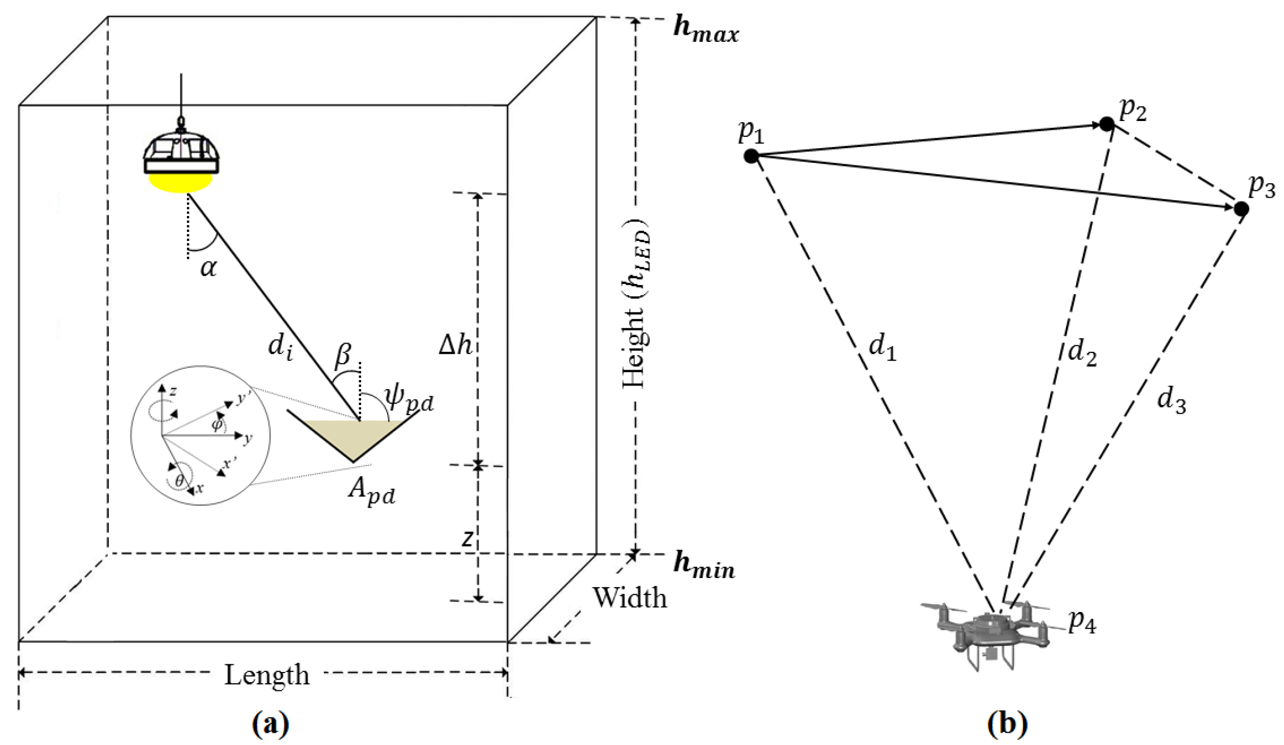
2.1. VLC System Model

Figure 1a shows the proposed environment with the flight path of the drone. It consisted of a typical industrial environment (25 m × 15 m × 5 m) with $N=15$ uniformly distributed LED based light fixtures with 5 m spacing between them. The N LED light fixtures were placed at a fixed height $h_{LED}$, with coordinates $(x_i,y_i,h_{LED})$, where $i=1...N$. We considered a receiver with an active area of $A_{pd}$ located at the unknown location $(x,y,z)$. Furthermore, various trajectories including rectangular and elliptical were considered for the flight path of the drone. However, after extensive simulations, the infinity (∞) shaped path was selected for further simulation, as shown in Figure 1b. This is because the selected path covered multiple heights for the receiver within the proposed industrial environment.

We also assumed that the receiver was able to distinguish signals from different transmitters using time-division multiplexing as in [12] and that the transmitters were synchronized. For typical LEDs with Lambertian radiation order m, the received optical power $P_{ri}$ from the $i^{\mathrm{th}}$ LED transmitter is given by [15]:

$$P_{ri}=\left\{\begin{array}{cc}{P}_{ti}\frac{(m+1)A_{pd}}{2\pi d_i^2}co{s}^m\left(\alpha \right)cos\left(\beta \right),& \beta \le {\psi }_{pd}\\ 0,& \beta >{\psi }_{pd}\end{array}\right.$$

(1)

where $P_{ti}$ is the transmitter’s power from the $i^{\mathrm{th}}$ LED transmitter, $d_i$ is the distance between the $i^{\mathrm{th}}$ LED transmitter and the receiver, $\alpha$ is the angle of irradiance, $\beta$ is the angle of incidence and ${\psi }_{pd}$ is the field-of-view (FOV) of the photodiode receiver, as shown in Figure 2a. Moreover, by assuming that $cos\left(\alpha \right)=cos\left(\beta \right)=\frac{h_{LED}-z}{d_i}=\frac{h}{d_i}$ for horizontally oriented and parallel N LED transmitters and receiver, the $\widehat{d_i}$ can be estimated from the received signal power $P_{ri}$ as [16]:

$$\widehat{d_i}=\sqrt[m+3]{\frac{\left(m+1\right)A_{pd}{P}_t{h}_i^{m+1}}{2\pi P_{ri}}}$$

(2)

where $h_i$$=h_{LED}-z$ is the unknown vertical height difference between LED${}_i$ and the receiver. Since $\widehat{d_i}$ is dependent on $\alpha$, this could lead to the same $P_{ri}$ values for different distances from the transmitter at different heights. Hence, the estimated distance $\widehat{d_i}$ cannot be directly calculated from $P_{ri}$ without accurately knowing h. Due to this, we generated a set of estimated distances $\widehat{d_i}$ for different receiver heights z ranging from a minimum height $h_{min}$ and maximum height $h_{max}\le h_{LED}$ with a height resolution of 1 mm.

However, the assumption that the transmitter and receiver planes are parallel to each other might not always hold for a mobile receiver, especially in the case of drones. In this case, the receiver could tilt, and the angle of incidence is determined by [10]:

$$cos\left({\beta }_{tilt}\right)=\frac{\left(x-x_i\right)cos\phi sin\theta +\left(y-y_i\right)sin\phi sin\theta +\left(z-z_i\right)cos\theta }{d}$$

(3)

where $z_i=h_{LED}$ and $\theta$ is the receiver’s tilting angle, which is the angle difference between the normal vector of the xy-plane and the normal vector of the receiver. $\phi$ is the azimuthal rotation angle, which is the angle difference between the x-axis and the orthogonal projection of the receiver’s normal vector on the xy-plane. Moreover, the received signal in (1) can be affected by the shot and thermal noise. Artificial lights or sunlight have a direct impact on the shot noise, resulting in a larger background current. We assumed that there was an indirect sunlight exposure with a background current of 740 $\mathsf{\mu }$A [17]. The total noise can be estimated using ${\sigma }_{noise}^2={\sigma }_{shot}^2+{\sigma }_{thermal}^2$, and the signal-to-noise ratio (SNR) is given by [18]:

$$SN{R}_i\left(dB\right)=10lo{g}_{10}\frac{{\left(R_r{P}_{ri}\right)}^2}{{\sigma }_{noise}^2}$$

(4)

where $R_r$ is the receiver’s responsivity. The main parameters to calculate the noise are provided in

Table 1. Summary of the system parameters.

Parameter	Value
Room Width × Length × Height	25 m × 15 m × 5 m
Walls’ Reflectivity	0.17
Floor’s Reflectivity	0.34
Transmitter’s Power, $P_t$	80 W
Transmitter’s Semi-Angle, $\alpha$	${45}^{\circ }$
Receiver’s Height, z	1.5–3.5 m
Photodetector Area, $A_{pd}$	1 cm${}^2$
Receiver’s FOV (Half Angle), ${\psi }_{pd}$	${80}^{\circ }$
Receiver’s Responsivity, $R_r$	0.54 A/W
Background Current, $I_{bg}$	740 $\mathsf{\mu }$A
Bandwidth, B	10 MHz

.

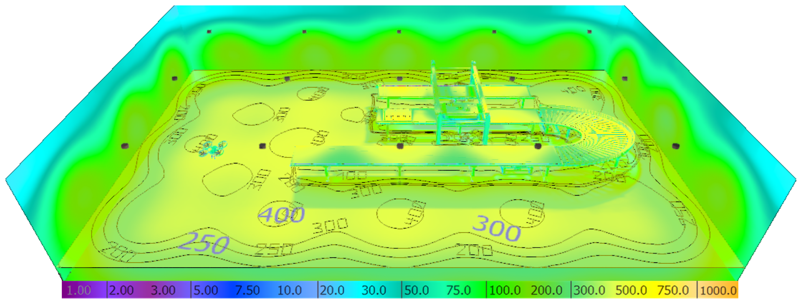
2.2. Illumination Levels

The minimum illumination requirement for industrial applications and typical workspaces for iron and steelwork with continuous manual labour is 200 lx based on European standards [19]. To ensure that these required illumination levels and coverage were met, simulations were performed using DIALux lighting design software [20]. The software allows the selection of different light fixtures from various light manufacturers for the design of optimum illumination levels. It also allows the selection of different types of surfaces that are made from a range of materials for indoor applications.

Figure 3 shows the illumination levels for the proposed industrial environment with a large conveyor belt placed in the middle of the factory floor. OSRAM’s PrevaLight High Bay LED based light fixtures were used with a power of 80 W and a ${45}^{\circ }$ semi-angle of divergence. These luminaires are suitable for industrial applications as they offer high power and wide beam distribution for a consistent coverage area that is typical in industrial environments [21].

Note that the floor material was considered to be fine concrete and had a reflection factor of 34%, and all the walls were red bricks with a reflection factor of 17%. The reflectivity coefficients were adopted from DIALux software to ensure its practicality. The simulation results showed that an average illumination of 270 lux was achieved around the entire area at the working plane height of 0.8 m. This verified that the selected light fixtures offered the minimum required illumination levels specified by the European standards and were suitable for industrial applications.

2.3. Positioning Algorithms

The positioning algorithm was performed by taking into account each set of estimated distances $\widehat{d_i}(i=1,...,N)$ using (2) for different heights of the receiver. Then, the unknown 3D position was estimated by using CMD and LLS by minimizing the cost function for the set of heights ranging from a minimum height $h_{min}$ and maximum height $h_{max}$.

2.3.1. Cayley–Menger Determinant

The novelty in our proposed method was the extension of CMD with a cost function to be used in VLP systems that enabled the estimation of a receiver’s 3D position without prior knowledge of its height. Figure 2b shows the position of three transmitters, $p1$, $p2$ and $p3$, with $p4$ being the unknown drone location. The CMD algorithm only required three transmitters to estimate a location; therefore, the corresponding signals from the three strongest (mostly the nearest) LEDs were taken into account, as they offered the highest SNR.

The Cayley–Menger bideterminant of two sequences of n points [$p_1,p_2,...,p_n$] and [$q_1,q_2,...,q_n]$ is defined as [22]:

$$D\left(p_1,...,p_n;q_1,...,q_n\right)=2{\left(\frac{-1}{2}\right)}^n\left|\begin{array}{ccccc}0& 1& 1& 1& 1\\ 1& D\left(p_1,q_1\right)& D\left(p_1,q_2\right)& \cdots & D\left(p_1,q_n\right)\\ 1& D\left(p_2,q_1\right)& D\left(p_2,q_2\right)& \cdots & D\left(p_2,q_n\right)\\ ⋮& ⋮& ⋮& \ddots & ⋮\\ 1& D\left(p_n,q_1\right)& D\left(p_n,q_2\right)& \cdots & D\left(p_n,q_n\right)\end{array}\right|$$

(5)

where $D(p_i,q_j)$ is the squared distance between points $p_i$ and $q_j$. When two sequences of points are the same (i.e., $p_i=q_i$), then $D(p_1,...,p_n;q_1,...,q_n)$ is denoted by $D(p_1,...,p_n)$ and is simply called CMD [22]. Assuming $p_4$ is the unknown location of the drone, $D(p_4,p_1)$, $D(p_4,p_2)$ and $D(p_4,p_3)$ are the distances $\widehat{d_1}$, $\widehat{d_2}$ and $\widehat{d_3}$ that are computed from the RSS for a given receiver height. It is then possible to calculate the unknown position of the receiver $\left(p_4\right)$ with respect to three known transmitter coordinates $(p_1,p_2,p_3)$ using [22]:

$$p_4=p_1+k_1{v}_1+k_2{v}_2\pm k_3\left(v_1{v}_2\right)$$

(6)

where $v_1=p_2-p_1$, $v_2=p_3-p_1$ and the ± sign accounts for the two mirror symmetric locations with respect to the base plane, but given the impossibility of a receiver being above the light fixtures, one of the possibilities can be ignored. $k_1$, $k_2$ and $k_3$ are given by:

$$k_1=-\frac{D(p_1,p_2,p_3;p_1,p_3,p_4)}{D(p_1,p_2,p_3)},k_2=\frac{D(p_1,p_2,p_3;p_1,p_2,p_4)}{D(p_1,p_2,p_3)},k_3=\frac{\sqrt{D(p_1,p_2,p_3,p_4)}}{D(p_1,p_2,p_3)}$$

The proposed algorithm then outputs $(\widehat{x}\left(h\right),\widehat{y}\left(h\right),\widehat{z}\left(h\right))$ for each of the assumed possible heights. Once all the possible receiver locations have been generated, the estimated location is found at the minimum of the cost function $C\left(h\right)$ as:

$$C\left(h\right)=\frac{1}{N}\sum _{i=1}^N{\left[\widehat{d_i}\left(h\right)-\sqrt{{\left(\widehat{x}\left(h\right)-x_i\right)}^2+{(\widehat{y}\left(h\right)-y_i)}^2+(\widehat{z}\left(h\right)-z_i)}\right]}^2$$

(7)

Here, $C\left(h\right)$ is the average squared error between the estimated distances $\widehat{d_i}$(h) using (2) and the distances of the estimated location $(\widehat{x}\left(h\right),\widehat{y}\left(h\right),\widehat{z}\left(h\right))$ using (6). After estimating the 3D position of the unknown receiver $\left(p_4\right)$, the final estimated position $(\widehat{x},\widehat{y},\widehat{z})$ is compared with the actual position of the receiver to find the positioning error as:

$$D_{error}=\sqrt{{\left(\widehat{x}-x\right)}^2+{\left(\widehat{y}-y\right)}^2+{\left(\widehat{z}-z\right)}^2}$$

(8)

2.3.2. Linear Least Squares

As the correct distances cannot be estimated directly without knowing the receiver’s height, 2D trilateration using LLS was performed for each of the assumed heights h. The horizontal squared distance between the $N$ LED transmitter and a receiver is given by:

$$d_i^2\left(h\right)={(x_i-x)}^2+{(y_i-y)}^2=x^2-2x{x}_i+x_i^2+y^2-2y{y}_i+y_i^2$$

(9)

These linear equations can be expressed in a matrix form as $b=A\mathbf{x}$, where:

$$b=\frac{1}{2}\left[\begin{array}{c}{d}_1^2\left(h\right)-x_1^2-y_1^2-d_N^2\left(h\right)+x_N^2+y_N^2\\ d_2^2\left(h\right)-x_2^2-y_2^2-d_N^2\left(h\right)+x_N^2+y_N^2\\ ⋮\\ d_{N-1}^2\left(h\right)-x_{N-1}^2-y_{N-1}^2-d_N^2\left(h\right)+x_N^2+y_N^2\end{array}\right]$$

(10)

$$A=\left[\begin{array}{cc}{x}_1-x_N& y_1-y_N\\ x_2-x_N& y_2-y_N\\ ⋮& ⋮\\ x_{N-1}-x_N& y_{N-1}-y_N\end{array}\right],\mathbf{x}=\left[\begin{array}{c}x\\ y\end{array}\right]$$

(11)

The algorithm then outputs the estimated position $\left[\begin{array}{c}\widehat{x}\\ \widehat{y}\end{array}\right]$ for each of the assumed possible heights h using the Moore–Penrose pseudo-inverse of A:

$$\mathbf{x}={\left(A^{T}A\right)}^{-1}{A}^{T}b$$

(12)

After that, minimization is achieved by using (7) in order to find the most probable 3D position as in our previous work in [23].

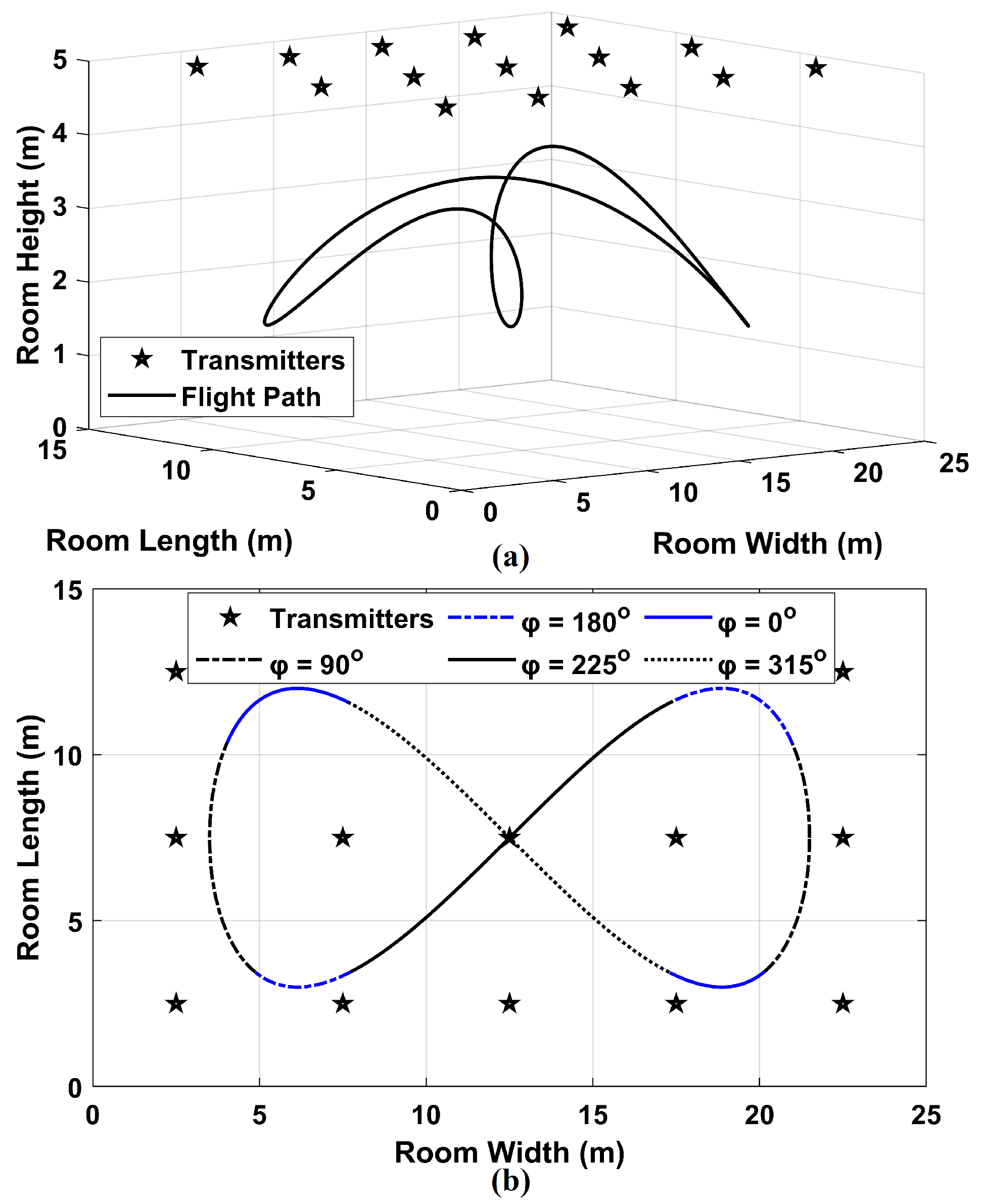
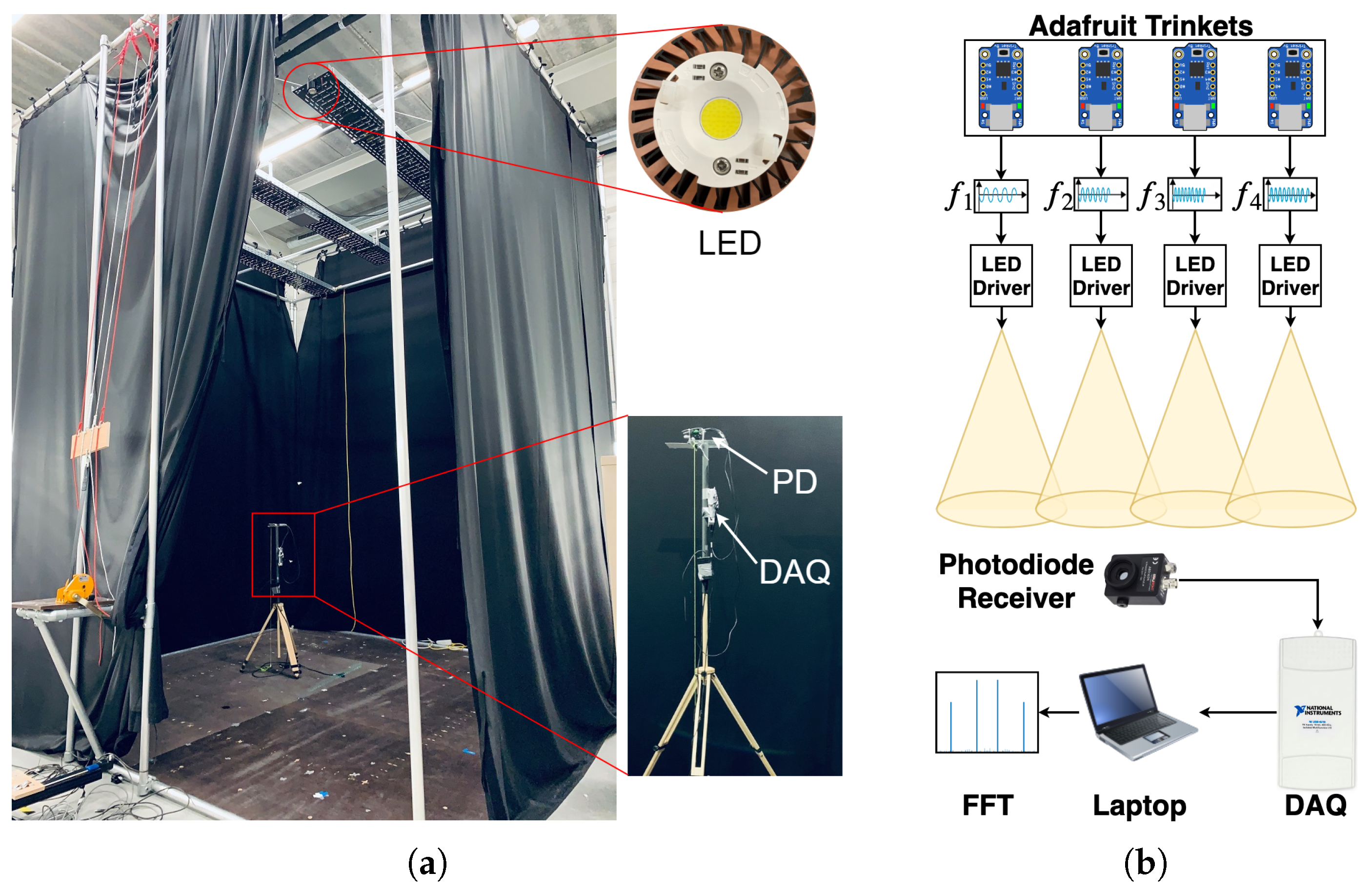
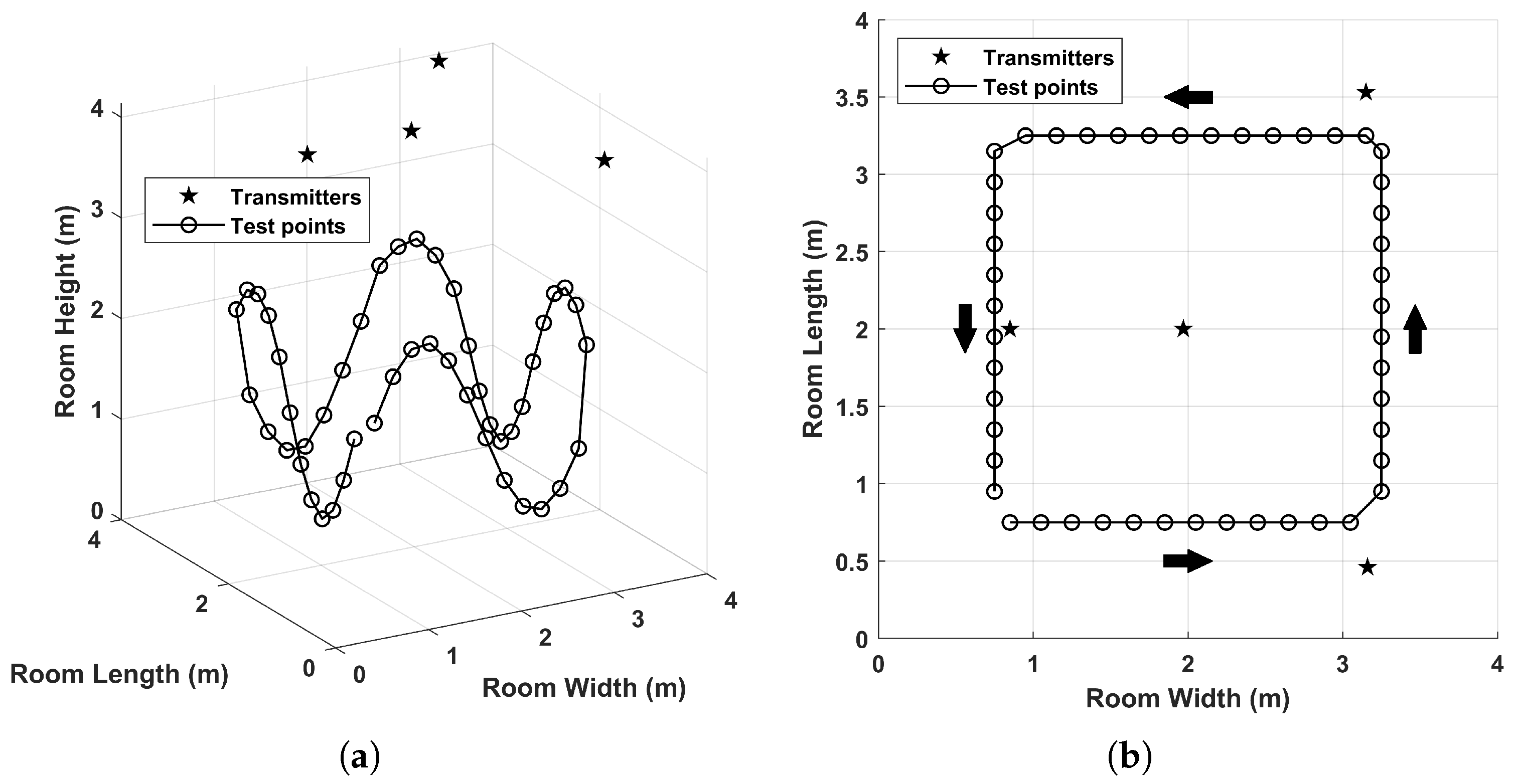
2.3.3. Experimental Validation: Configuration

To validate our proposed algorithm, we experimentally tested our method in a VLP lab measuring 4 m × 4 m with the height of the LEDs at approximately 4.1 m, as shown in Figure 4a. The transmitters used were BXRE-50C3001-D-24 LEDs and were intensity-modulated using pulse trains with a duty cycle of 0.5 with frequencies of 500 Hz, 1 kHz, 2 kHz and 4 kHz, generated using Adafruit Trinkets. This ensured that the received signals from the different LEDs could be demultiplexed individually at the receiver side. The LEDs were placed in a star configuration due to the ambiguity that occurs when only four LEDs are used in a square configuration, as demonstrated in our previous work in [23].

The Thorlabs PDA36A2 optical receiver had an integrated electrical amplifier with an active area $A_{pd}$ of 13 mm${}^2$. The photodiode’s responsivity was obtained by weighing the responsivity curve of the photodiode over the wavelength dependence of the LED and calculating an estimated value of 0.22 A/W. The receiver was attached to a tripod with a vertical pole that allowed adjustment of the receiver’s height, as shown in Figure 4a. The current was digitized using National Instrument’s USB-6212 DAQ device. A fast Fourier transform (FFT) based demodulation was used to extract the received power values for each LED in MATLAB^®, as specified in [24]. A block diagram of the experimental setup is also shown in Figure 4b.

The measurements were taken in the VLP test bed as shown in Figure 5. The selected path took the receiver around the room at different heights ranging from 0.64 to 2.55 m, as shown in Figure 5a. Here, we considered forty-eight test points for the selected path, and twenty-five measurements were taken at each location. A top view of the experimental path within the VLP test bed and the locations of the LEDs are also shown in Figure 5b.

3. Results and Discussion

The performance of the proposed CMD algorithm was evaluated in terms of positioning error for a typical industrial deployment, adhering to the standardized illumination levels, by considering (i) normal line-of-sight and untilted reception, (ii) different tilt angles of the receiver and (iii) multipath reflections. The main simulation parameters are summarized in Table 1.

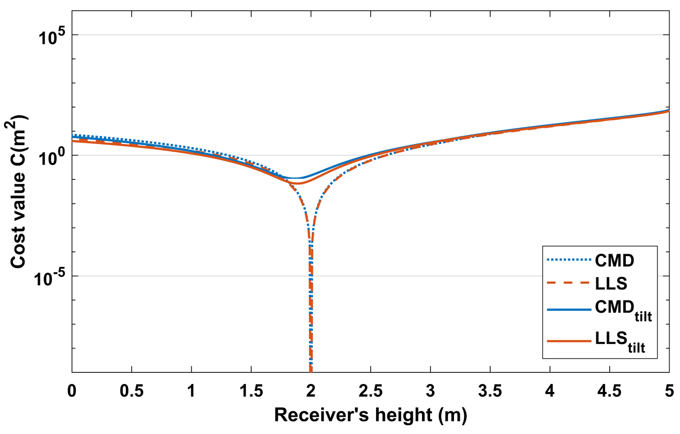
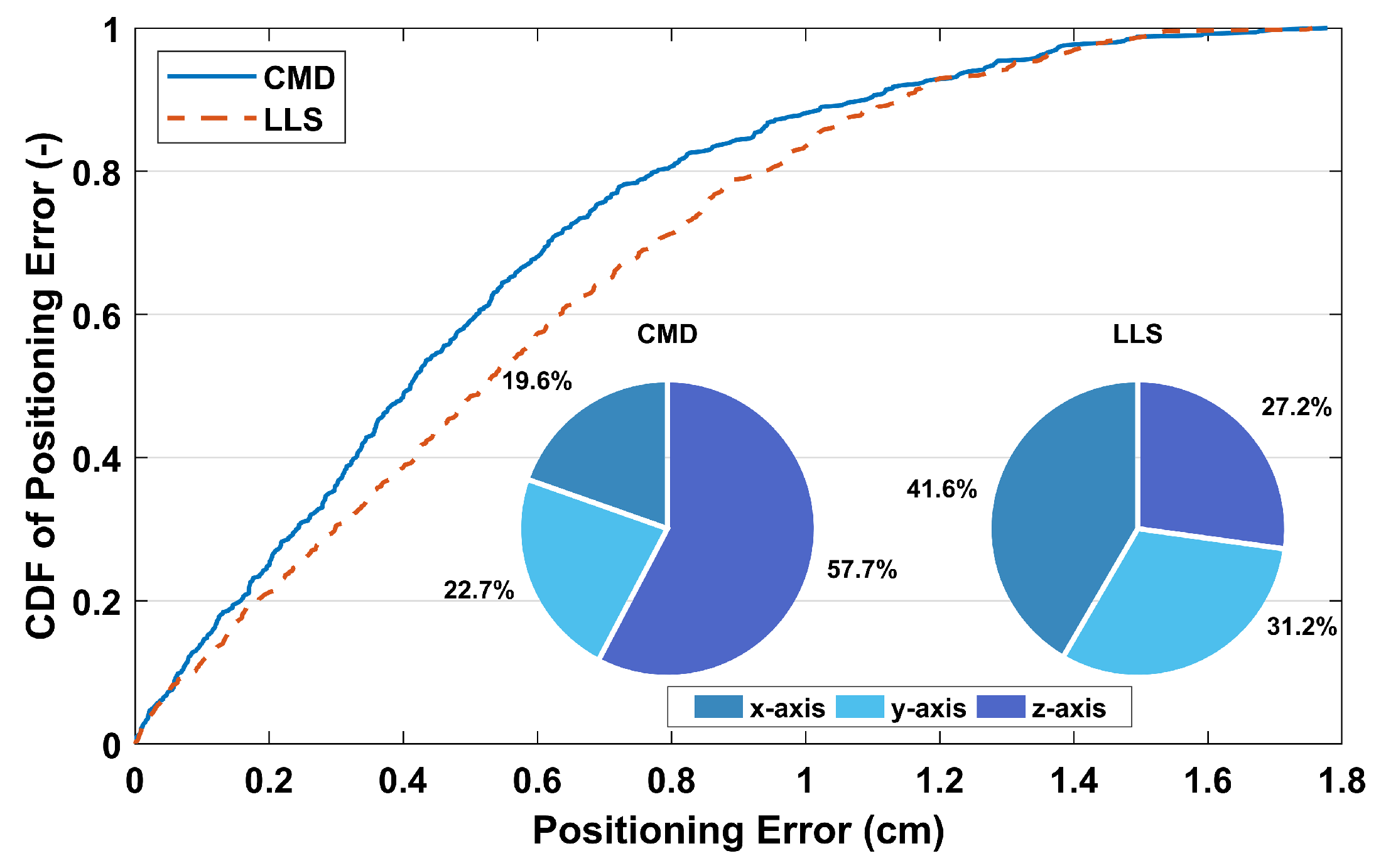
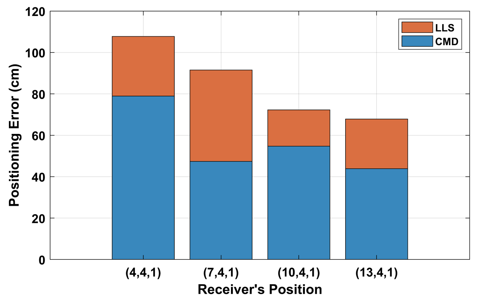
3.1. Positioning Accuracy for Line-of-Sight Reception with Untilted Receiver

The performance of the algorithm was first evaluated to investigate the effect of tilt on the height estimation using the RSS and cost function for a position when the receiver was at (10 m, 6 m, 2 m). Figure 6 shows the value of the cost function as a function of the receiver’s height with and without the effect of tilt for both the CMD and LLS algorithms.

The result showed that without tilt, the cost function minimized at h = 2 m for CMD and LLS, i.e., the estimated height of the receiver and the actual height were the same. This verified that the estimated height was very precise due to the high SNR values (>34 dB) using (4). However, for a tilt angle, $\theta$ = $5^{\circ }$, the estimated height was 1.82 m when CMD was used and 1.89 m for LLS. This showed the adverse effect of tilt on the estimation of height h using RSS.

Furthermore, a realistic flight path was considered using a set of 500 points around the manufacturing environment, as shown in Figure 1. This path was selected to take the drone around most of the room with varying heights ranging from 1.5 to 3.5 m. The estimated SNR values for the selected flight path ranged from a maximum of 82.8 dB to 19.2 dB when the drone was at (12.5, 7.5, 3.5), which was directly under the LED light fixture in the centre of the room; see Figure 1b. Note that these high SNR values for VLP were due to the high power LEDs and the adherence to the minimum illumination constraint, as also reported in [25,26,27].

Figure 7 shows the cumulative distribution function (CDF) of the positioning errors for the 500 points. The positioning errors along the path were evaluated using (8). The results in Figure 7 show small positioning errors and high accuracy, which was similar as reported in experiments and simulations [28]. It can be observed that around 80% of the points had a positioning error less than 0.78 cm for CMD and 0.94 cm for LLS. Half of the errors (50%) using CMD and LLS were below 0.42 cm and 0.52 cm, respectively. Due to the fact that LLS used all of the received signals including signals from far-away LEDs, SNR values as low as 1.04 dB were measured at some locations. This can introduce higher positioning errors than the CMD algorithm, which required only three LED transmitters. The CMD outperformed the LLS algorithm by an average of 14%, and the median was improved by 23%. A breakdown of the errors for the three different axes is shown in Figure 7 (see the inset). The majority (57.7%) of the positioning errors using CMD were comprised of vertical error (z-axis), while the x- and y-axis errors were 19.6% and 22.7%, respectively. However, the main part of the error using the LLS method was mostly horizontal error with 41.6% from the y-axis and 31.2% from the x-axis. Contrarily, the z-axis was the smallest contributor with around 27.2% of the total positioning error.

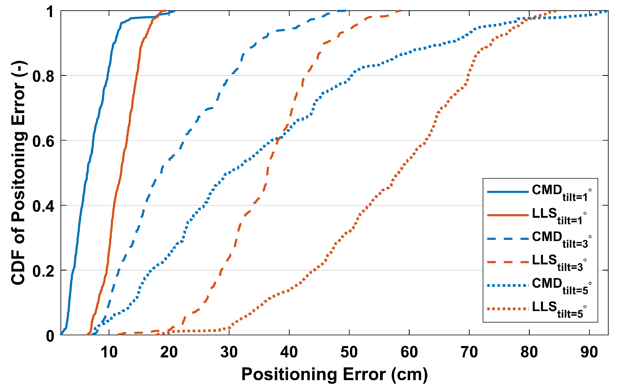
3.2. The Effect of Tilting

A widespread assumption made in the literature for VLP systems is that the transmitter and receiver are parallel, as assumed in (2). However, this assumption does not hold in real-world applications, where the moving drone tilts in order to move forward at different azimuthal angles, as shown in Figure 1b. Therefore, the effect of tilting was investigated here. The tilt of the drone was set to a forward tilt angle $\theta$ with values of $1^{\circ }$, $3^{\circ }$ and $5^{\circ }$, and the value of the azimuthal angle $\phi$ changed along the path; see Figure 1b. In our model, the receiver faced the eastern wall when $\phi$ = $0^{\circ }$ and the northern wall when $\phi$ = ${90}^{\circ }$. Therefore, changing the azimuthal angle during the flight path ensured that the drone was always forward-facing. Noise was not considered here in order to analyse the effect of tilt and azimuthal angles on the positioning accuracy independently.

Figure 8 shows the CDF of the positioning error for the 500 points for the selected path with $\theta$ = $1^{\circ }$, $3^{\circ }$ and $5^{\circ }$ for the proposed CMD algorithm. The performance of the proposed CMD algorithm was also compared with the benchmark LLS algorithm. A clear increase in the positioning error was noticed for all the tilt angles, $\theta$ = $1^{\circ }$, $3^{\circ }$ and $5^{\circ }$. It was observed that for $\theta$ = $1^{\circ }$, the median errors were 6.4 cm and the maximal (95%) errors were 12 cm when CMD was used, while the median errors were 12 cm and the maximal errors were 16.8 cm when LLS was used. Similarly, for $\theta$ = $3^{\circ }$, CMD achieved a median error of 18.6 cm and a maximal of 41.3 cm, while LLS had median and maximal errors of 36.4 cm and 50.6 cm, respectively. For $\theta$ = $5^{\circ }$, the median and maximal errors for CMD were 30 cm and 72.2 cm and 58.2 and 77.7 cm for LLS. It was also noticed that the CMD algorithm had a few points with errors higher than LLS. However, CMD outperformed the LLS VLP algorithm with a median error difference of 5.6 cm, 17.8 cm and 28.2 cm for $\theta$ = $1^{\circ }$, $3^{\circ }$ and $5^{\circ }$, respectively.

It should be noted that the severity of the tilting effect is also dependent on the user, as the operator can adjust the maximum tilt angle when initializing the drone. Additionally, the effect of the receiver tilt could be simply alleviated by using a compensation method such as the one proposed in [14], where the effect of the tilts was compensated using on-board sensors such as a gyroscope that reduced the positioning error from 60.4 cm to 1.62 cm after the compensation. Another method to alleviate the effect of tilt is by keeping the drone horizontal and tilting the rotors for movement [29].

3.3. Positioning Accuracy with Multipath Reflections

The effect of multipath reflections was also investigated for the proposed CMD algorithm and the LLS algorithm. The position of the receiver was considered at (4,4,1), (7,4,1), (10,4,1) and (13,4,1) in order to test the effect of multipath reflections. These positions were selected as they covered the multipath reflections due to their position close to the walls and up to the middle of the room, i.e., the effect of high to low multipath reflections. The channel impulse response was simulated for the selected positions using the modified Monte Carlo ray tracing method outlined in [30], and up to three reflections were taken into account, as these contained the majority of the signal power. In order to analyse the effect of multipath reflections only, noise was not considered in these simulations. Furthermore, the wall and floor reflectivity coefficients were considered based on the concrete and red brick materials to mimic a real indoor industrial environment; see Table 1.

Figure 9 shows the positioning errors for the four specified locations of the receiver with multipath reflections. The results showed that when the receiver was at (4, 4, 1), and LLS achieved a positioning error of 107 cm, while CMD had an error of 79 cm. When the receiver was at (7,4,1), (10,4,1) and (13,4,1), the positioning error for LLS was 91.53 cm, 72.24 cm and 67.85 cm, respectively, while the CMD achieved a positioning error of 47.36 cm, 54.72 cm and 43.84 cm, respectively. Therefore, the performance of CMD was superior to that of LLS in the presence of multipath reflections. This was due to the fact that LLS used any number of signals that were received by the receiver along with their corresponding reflections, meaning that it had more skewed signals, which had a compounding effect. Hence, the receiver’s position estimation was affected by the multipath reflections from those signals, as well, especially given that the reflections contributed significantly more to the received power when coming from farther transmitters due to larger room dimensions. However, this effect was less severe in CMD as the algorithm only selected the strongest three signals to find a position. Likewise, a higher positioning error of 170 cm was also reported in [12] due to multipath reflections even for 2D localization, albeit for smaller room dimensions. A method to reduce the effect of the multipath reflections was proposed in [31]. The authors proposed the use of orthogonal frequency division multiplexing (OFDM) to mitigate the effect of multipath reflections and to provide high data rate transmissions. Their results reported a root mean squared (RMS) error of 0.04 m when OFDM modulation was used, while it was 0.43 m for when on-off keying (OOK) modulation was used.

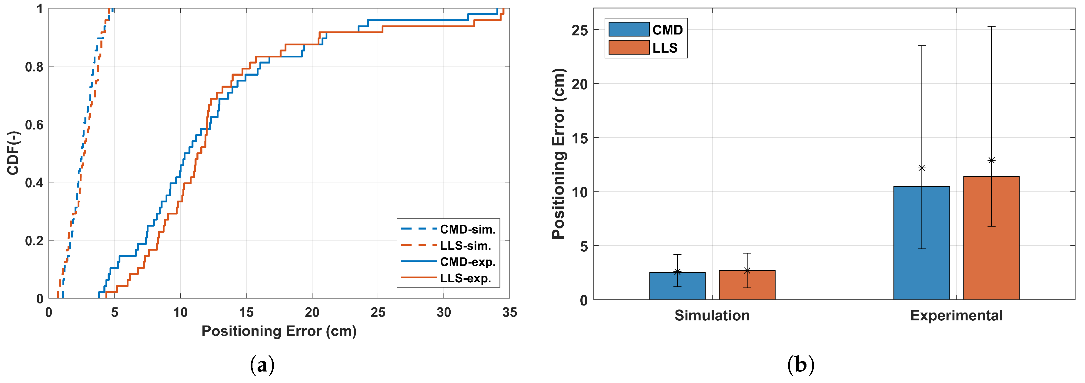
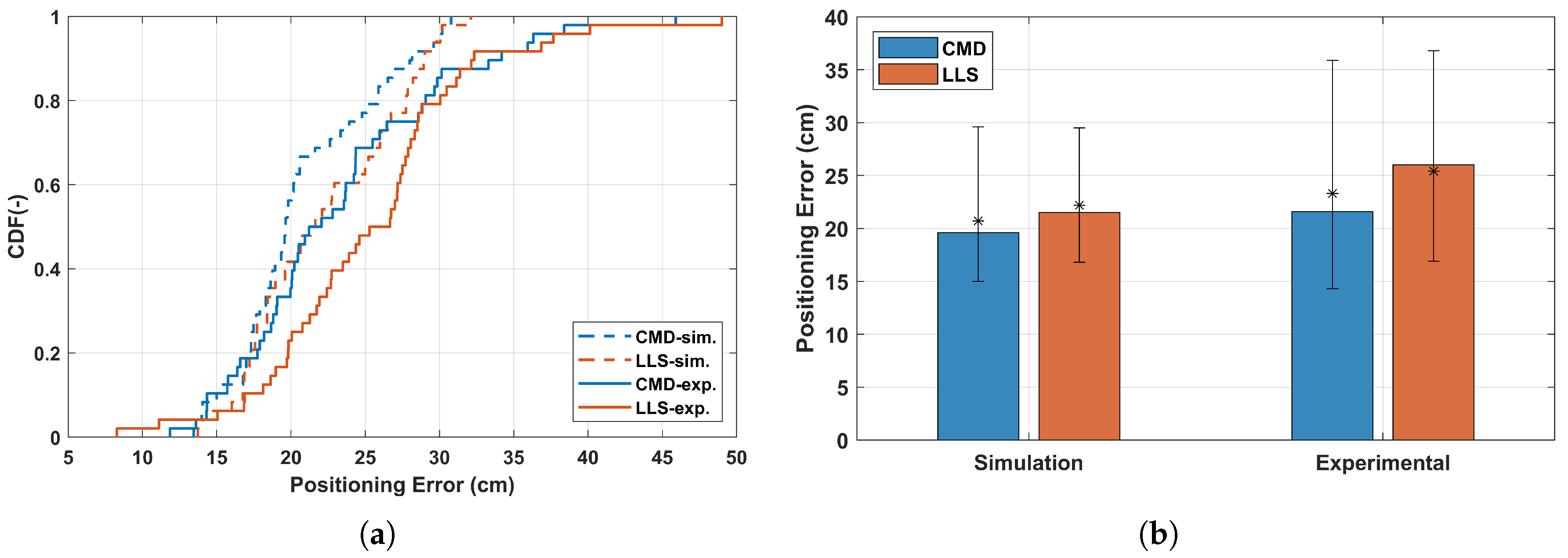
3.4. Experimental Validation

Our proposed algorithm was experimentally tested based on the specifications detailed in Section 2.3.3. Figure 10a shows the CDF of the simulation and measured positioning errors for the CMD and LLS algorithms. The results showed that the median and maximal errors for the CMD were 10.5 and 23.2 cm, while the median and maximal errors for the LLS were 11.4 and 25.3 cm. However, the simulation results showed that the median and maximal errors for the CMD were 2.5 and 4.2 cm, while the median and maximal errors for the LLS algorithm were 2.7 and 4.3 cm. Furthermore, the simulation and measured average errors are represented as an asterisk for both the algorithms, and the 10% and 90% quantiles are shown in Figure 10b. The results show that the measured average error for the CMD algorithm was 12.2 cm, while the measured average error for LLS was 12.9 cm. The average error for the simulations was almost comparable to the CMD and LLS algorithms. Note that the experimental median error in CMD was lower than the LLS algorithm by 8%. A summary of the median, maximal and average errors for CMD and LLS algorithms for the simulations and experiment results is shown in

Table 2. The simulation and experimental positioning errors for the CMD and LLS algorithms in simulation and experimentally when the receiver was horizontal and had a receiver tilt of ${10}^{\circ }$.

Positioning Error (cm)	LLS			CMD
	${\mathit{p}}_{\mathbf{50}}$	${\mathit{p}}_{\mathbf{90}}$	$\mathit{m}$	${\mathit{p}}_{\mathbf{50}}$	${\mathit{p}}_{\mathbf{90}}$	$\mathbf{mean}$
Simulation $(\theta =0^{\circ })$	2.7	4.3	2.7	2.5	4.2	2.6
Experimental $(\theta =0^{\circ })$	11.4	25.3	12.9	10.5	23.5	12.2
Simulation $(\theta ={10}^{\circ })$	21.5	29.5	22.2	19.6	29.6	20.7
Experimental $(\theta ={10}^{\circ })$	26	36.8	25.4	21.6	35.9	23.3

.

In order to validate the simulations for the CMD and LLS algorithms for the effect of tilting, the experimental test was repeated for the same path with a receiver tilt $\theta ={10}^{\circ }$, as shown in Figure 5a. Figure 11a shows the CDF of the measured and simulation position error for the CMD and LLS algorithm with receiver tilt. The experimental results showed that the median and maximal errors for CMD were 21.6 and 35.9 cm, while the measured median and maximal error for LLS were 26.0 and 36.8 cm. However, the simulation results showed that the median and maximal errors for the CMD were 19.6 and 29.5 cm, and similarly, the median and maximal errors for the LLS were 21.5 and 29.6 cm. The measured average position error for the CMD was 23.3 cm, and similarly, the measured average position error for the LLS was 25.4 cm. However, the simulation results showed the average position error of 20.7 cm for the CMD algorithm and 22.2 cm for the LLS algorithm. This showed a good agreement between the simulation and experimental CDF of the positioning error for both the CMD and LLS algorithms. The experimental results also showed that an average error in CMD was lower by 8.6% than the LLS algorithm. Furthermore, a summary of the median, maximal and average errors with receiver tilt $\theta ={10}^{\circ }$ for the CMD and LLS algorithms is also shown in Table 2.

The experimental results reached the same conclusion as the simulation results and demonstrated the applicability of our algorithm for 3D positioning without prior knowledge of the receiver’s height. It should be noted that some of the errors observed in our experiments could also be caused by other factors such as (i) the LEDs having small unknown tilt angles [32], (ii) the LED radiation pattern not being perfectly Lambertian and (iii) the LED power showing a deviation from their advertised values [33]. The difference between the simulated and experimental results was due to the nature of experimental work and background noise. Similar discrepancies in experimentally tested VLP systems were reported in [7], where simulation results reported an average error of 3.9 mm and their achieved experimental errors were 3.5 cm. Similarly, the work in [8] reported an average simulation accuracy of 1.12 cm at a receiver height of 1 m and a positioning accuracy within 10 cm when the receiver was at a height of 0.75 m.

4. Conclusions

In this paper, a new and simple algorithm for 3D VLP based on the RSS was proposed and experimentally tested. The proposed method combined the use of the CMD trilateration algorithm with a cost function and was shown to be more accurate and robust when compared with the widely used LLS algorithm. The algorithm’s performance was shown for a drone travelling a realistic path in a manufacturing environment, and the positioning error was simulated with and without the impact of tilt and multipath reflections. The results showed that the proposed CMD VLP algorithm outperformed the LLS algorithm by an average of 14% and a median improvement of 21% without receiver tilt or multipath reflections. When a receiver tilt of $5^{\circ }$ was considered, CMD achieved median and maximal errors of 30 cm and 72.2 cm, while LLS achieved median and maximal errors of 58.2 and 77.7 cm. Furthermore, the effect of multipath reflection was also investigated with the CMD algorithm, achieving an error of 79 cm, while the LLS algorithm achieved an error of 107 cm when the receiver was close to a wall. The proposed algorithm was also tested in a test bed measuring 4 × 4 × 4.1 m${}^3$. The experimental results also showed that the proposed CMD algorithm with the cost function achieved a median error of 10.5 cm, while LLS achieved a median error of 11.4 cm. This shows that the CMD with a cost function algorithm was more accurate than the LLS trilateration method and the use of the cost function could estimate the 3D position of a receiver without prior knowledge of its height, eliminating the need for additional sensors.

References

1. Jordan, S.; Moore, J.; Hovet, S.; Box, J.; Perry, J.; Kirsche, K.; Lewis, D.; Tse, Z.T.H. State-of-the-art technologies for UAV inspections. IET Radar Sonar Navig. 2018, 12, 151–164. [Google Scholar] [CrossRef]
2. Benini, A.; Mancini, A.; Longhi, S. An IMU/UWB/Vision-based Extended Kalman Filter for Mini-UAV Localization in Indoor Environment using 802.15.4a Wireless Sensor Network. J. Intell. Robot. Syst. 2013, 70, 461–476. [Google Scholar] [CrossRef]
3. Wu, K.J.; Gregory, T.S.; Moore, J.; Hooper, B.; Lewis, D.; Tse, Z.T.H. Development of an indoor guidance system for unmanned aerial vehicles with power industry applications. IET Radar Sonar Navig. 2017, 11, 212–218. [Google Scholar] [CrossRef]
4. Soria, P.R.; Palomino, A.F.; Arrue, B.C.; Ollero, A. Bluetooth network for micro-uavs for communication network and embedded range only localization. In Proceedings of the International Conference on Unmanned Aircraft Systems (ICUAS), Miami, FL USA, 13–16 June 2017; pp. 747–752. [Google Scholar] [CrossRef]
5. Ueyama, J.; Freitas, H.; Faical, B.S.; Filho, G.P.R.; Fini, P.; Pessin, G.; Gomes, P.H.; Villas, L.A. Exploiting the use of unmanned aerial vehicles to provide resilience in wireless sensor networks. IEEE Commun. Mag. 2014, 52, 81–87. [Google Scholar] [CrossRef]
6. Yasir, M.; Ho, S.W.; Vellambi, B.N. Indoor Positioning System Using Visible Light and Accelerometer. J. Lightwave Technol. 2014, 32, 3306–3316. [Google Scholar] [CrossRef]
7. Cai, Y.; Guan, W.; Wu, Y.; Xie, C.; Chen, Y.; Fang, L. Indoor High Precision Three-Dimensional Positioning System Based on Visible Light Communication Using Particle Swarm Optimization. IEEE Photonics J. 2017, 9, 1–20. [Google Scholar] [CrossRef]
8. Zhang, M.; Li, F.; Guan, W.; Wu, Y.; Xie, C.; Peng, Q.; Liu, X. A three-dimensional indoor positioning technique based on visible light communication using chaotic particle swarm optimization algorithm. Optik 2018, 165, 54–73. [Google Scholar] [CrossRef]
9. Chen, H.; Guan, W.; Li, S.; Wu, Y. Indoor high precision three-dimensional positioning system based on visible light communication using modified genetic algorithm. Opt. Commun. 2018, 413, 103–120. [Google Scholar] [CrossRef]
10. Yang, S.; Kim, H.; Son, Y.; Han, S. Three-Dimensional Visible Light Indoor Localization Using AOA and RSS With Multiple Optical Receivers. J. Lightwave Technol. 2014, 32, 2480–2485. [Google Scholar] [CrossRef]
11. Gu, W.; Zhang, W.; Kavehrad, M.; Feng, L. Three-dimensional light positioning algorithm with filtering techniques for indoor environments. Opt. Eng. 2014, 53, 107107. [Google Scholar] [CrossRef]
12. Gu, W.; Aminikashani, M.; Deng, P.; Kavehrad, M. Impact of Multipath Reflections on the Performance of Indoor Visible Light Positioning Systems. J. Lightwave Technol. 2016, 34, 2578–2587. [Google Scholar] [CrossRef]
13. Tang, W.; Zhang, J.; Chen, B.; Liu, Y.; Zuo, Y.; Liu, S.; Dai, Y. Analysis of indoor VLC positioning system with multiple reflections. In Proceedings of the 16th International Conference on Optical Communications and Networks (ICOCN), Wuzhen, China, 7–10 August 2017; pp. 1–3. [Google Scholar] [CrossRef]
14. Jeong, E.; Yang, S.; Kim, H.; Han, S. Tilted receiver angle error compensated indoor positioning system based on visible light communication. Electron. Lett. 2013, 49, 890–892. [Google Scholar] [CrossRef]
15. Kahn, J.M.; Barry, J.R. Wireless infrared communications. Proc. IEEE 1997, 85, 265–298. [Google Scholar] [CrossRef]
16. Plets, D.; Eryildirim, A.; Bastiaens, S.; Stevens, N.; Martens, L.; Joseph, W. A Performance Comparison of Different Cost Functions for RSS-Based Visible Light Positioning Under the Presence of Reflections. In Proceedings of the 4th ACM Workshop on Visible Light Communication Systems, Snowbird, UT, USA, 16 October 2017; pp. 37–41. [Google Scholar]
17. Moreira, A.J.C.; Valadas, R.T.; de Oliveira Duarte, A.M. Optical Interference Produced by Artificial Light. Wirel. Netw. 1997, 3, 131–140. [Google Scholar] [CrossRef]
18. Ghassemlooy, Z.; Popoola, W.; Rajbhandari, S. Optical Wireless Communications: System and Channel Modelling With Matlab; CRC Press: Boca Raton, FL, USA, 2017. [Google Scholar]
19. de Normalisation, C.E. EN 12464-1: Light and Lighting-Lighting of Work Places, Part 1: Indoor Work Places; Comité Européen de Normalisation: Brussels, Belgium, 2002. [Google Scholar]
20. DIAL. DIALux. Available online: https://www.dial.de/en/dialux/ (accessed on 7 November 2019).
21. Almadani, Y.; Ijaz, M.; Rajbhandari, S.; Adebisi, B.; Raza, U. Application of Visible Light Communication in an Industrial Environment. In Proceedings of the 11th International Symposium on Communication Systems, Networks & Digital Signal Processing (CSNDSP), Budapest, Hungary, 18–20 July 2018; pp. 1–6. [Google Scholar] [CrossRef]
22. Thomas, F.; Ros, L. Revisiting trilateration for robot localization. IEEE Trans. Robot. 2005, 21, 93–101. [Google Scholar] [CrossRef] [Green Version]
23. Plets, D.; Almadani, Y.; Bastiaens, S.; Ijaz, M.; Martens, L.; Joseph, W. Efficient 3D trilateration algorithm for visible light positioning. J. Opt. 2019, 21, 05LT01. [Google Scholar] [CrossRef]
24. De Lausnay, S.; De Strycker, L.; Goemaere, J.; Stevens, N.; Nauwelaers, B. A Visible Light Positioning system using Frequency Division Multiple Access with square waves. In Proceedings of the 2015 9th International Conference on Signal Processing and Communication Systems (ICSPCS), Cairns, Australia, 14–16 December 2015; pp. 1–7. [Google Scholar] [CrossRef]
25. Fath, T.; Haas, H. Performance Comparison of MIMO Techniques for Optical Wireless Communications in Indoor Environments. IEEE Trans. Commun. 2013, 61, 733–742. [Google Scholar] [CrossRef]
26. Al-Kinani, A.; Wang, C.; Haider, F.; Haas, H.; Zhang, W.; Cheng, X. Light and RF dual connectivity for the next generation cellular systems. In Proceedings of the IEEE/CIC International Conference on Communications in China (ICCC), Qingdao, China, 22–24 October 2017; pp. 1–6. [Google Scholar] [CrossRef]
27. Zeng, L.; Brien, D.O.; Le-Minh, H.; Lee, K.; Jung, D.; Oh, Y. Improvement of Date Rate by using Equalization in an Indoor Visible Light Communication System. In Proceedings of the 4th IEEE International Conference on Circuits and Systems for Communications, Shanghai, China, 26–28 May 2008; pp. 678–682. [Google Scholar] [CrossRef]
28. Luo, J.; Fan, L.; Li, H. Indoor Positioning Systems Based on Visible Light Communication: State of the Art. IEEE Commun. Surv. Tutor. 2017, 19, 2871–2893. [Google Scholar] [CrossRef]
29. Bin Junaid, A.; Diaz De Cerio Sanchez, A.; Betancor Bosch, J.; Vitzilaios, N.; Zweiri, Y. Design and Implementation of a Dual-Axis Tilting Quadcopter. Robotics 2018, 7, 65. [Google Scholar] [CrossRef]
30. Francisco, J. Lopez-Hernandez, Rafael Perez-Jimenez, A.S. Ray-tracing algorithms for fast calculation of the channel impulse response on diffuse IR wireless indoor channels. Opt. Eng. 2000, 39, 2775–2780. [Google Scholar] [CrossRef]
31. Aminikashani, M.; Gu, W.; Kavehrad, M. Indoor positioning with OFDM Visible Light Communications. In Proceedings of the 2016 13th IEEE Annual Consumer Communications Networking Conference (CCNC), Las Vegas, NV, USA, 9–12 January 2016; pp. 505–510. [Google Scholar] [CrossRef]
32. Plets, D.; Bastiaens, S.; Martens, L.; Joseph, W. An Analysis of the Impact of LED Tilt on Visible Light Positioning Accuracy. Electronics 2019, 8, 389. [Google Scholar] [CrossRef]
33. Plets, D.; Bastiaens, S.; Martens, L.; Joseph, W.; Stevens, N. On the impact of LED power uncertainty on the accuracy of 2D and 3D Visible Light Positioning. Optik 2019, 195, 163027. [Google Scholar] [CrossRef]
Figure 1. (a) The evaluated industrial environment showing the location of the LED light fixtures and the flight path of the drone; (b) a top view of the evaluated environment showing the azimuthal angles (rotation) φ along the entire path of the drone’s flight.
Electronics 08 01311 g001
Figure 2. (a) The VLP system block diagram; (b) the schematic diagram for the CMD trilateration problem and its parameters.
Electronics 08 01311 g002
Figure 3. Illumination levels for the selected environment under consideration.
Electronics 08 01311 g003
Figure 4. (a) The VLP lab where the experiments were conducted showing the LED and tripod used with the receiver and the DAQ unit highlighted; (b) a block diagram of the experimental setup.
Electronics 08 01311 g004
Figure 5. (a) A 3D view of the path of the receiver for the experimental test; (b) a top view of the evaluated path with the locations of the LEDs.
Electronics 08 01311 g005
Figure 6. Cost function showing the minimum at the receiver height when the receivers are parallel and tilted at an angle of θ = 5 .
Electronics 08 01311 g006
Figure 7. The CDF of errors for the flight path for the CMD and LLS algorithms. The inset shows a breakdown of the total positioning error for each axis for CMD and LLS.
Electronics 08 01311 g007
Figure 8. The CDF of errors for the flight path for CMD and LLS with tilt, θ values of 1 , 3 and 5 .
Electronics 08 01311 g008
Figure 9. The simulated positioning errors due to multipath reflections for selected positions using the CMD and LLS algorithms.
Electronics 08 01311 g009
Figure 10. (a) The CDF of the errors obtained in the experiment with a horizontal receiver; (b) the median errors with the 10% and 90% quantiles; the asterisk represents the mean error.
Electronics 08 01311 g010
Figure 11. (a) The CDF of the errors obtained in the experiment with a receiver tilted θ = 10 ; (b) the distribution of the median errors with the 10% and 90% quantiles; the asterisk represents the mean error.
Electronics 08 01311 g011