Elderly Fall Detection with an Accelerometer Using Lightweight Neural Networks

Abstract

Falls have been one of the main threats to people’s health, especially for the elderly. Detecting falls in time can prevent the long lying time, which is extremely fatal. This paper intends to show the efficacy of detecting falls using a wearable accelerometer. In the past decade, the fall detection problem has been extensively studied. However, since the hardware resources of wearable devices are limited, designing highly accurate embeddable models with feasible computational cost remains an open research problem. In this paper, different types of shallow and lightweight neural networks, including supervised and unsupervised models are explored to improve the fall detection results. Experiment results on a large open dataset show that the lightweight neural networks proposed have obtained much better results than machine learning methods used in previous work. Moreover, the storage and computation requirements of these lightweight models are only a few hundredths of deep neural networks in literature. In tested lightweight neural networks, the best one is proved to be the supervised convolutional neural network (CNN) that can achieve an accuracy beyond 99.9% with only 441 parameters. Its storage and computation requirements are only 1.2 KB and 0.008 MFLOPs, which make it more suitable to be implemented in wearable devices with restricted memory size and computation power.

1. Introduction

The world is currently experiencing an unprecedented aging of the population [1]. It has been estimated that the population of elder people aged 60 and over will keep increasing rapidly and exceed three billion by 2100. Such a huge elder market will stimulate the development of the healthcare industry. Hence, providing healthcare service to the elder to reduce living risks associated with their daily life is increasingly being demanded.

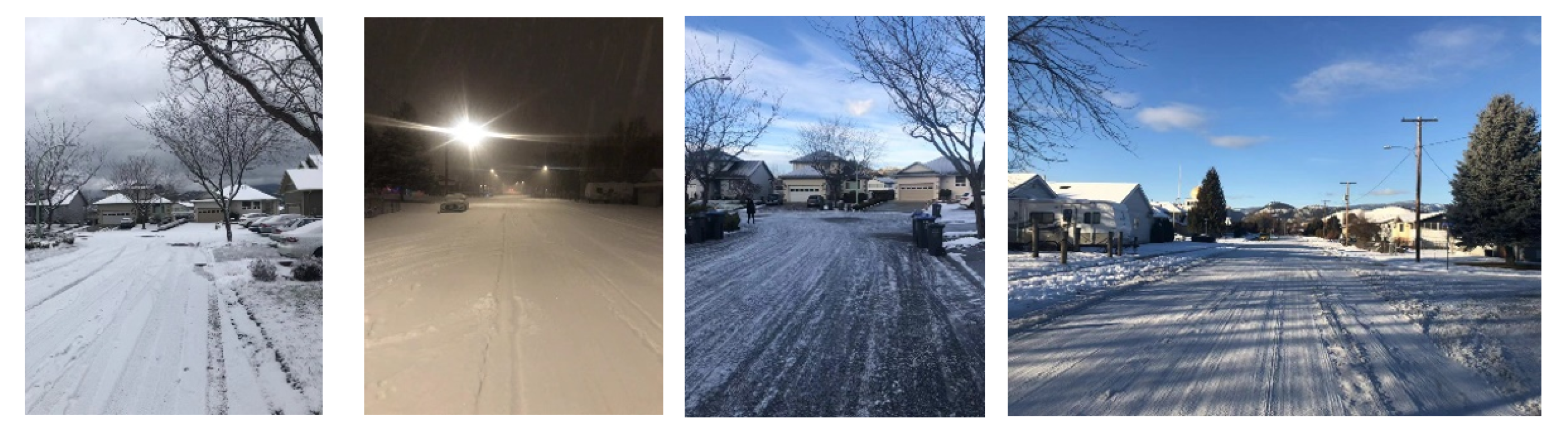
Meanwhile, falls have been one of the main threats in elder people’s life [2]. Almost 80% of reported accidents among elder patients are due to falls [3]. This situation is even worse in high altitude areas that are usually covered with snow and ice for most of the year, such as Canada, North America, and China. For instance, a living environment with a high risk of falling in Kelowna (Canada) is shown in Figure 1.

Early detection of falls can minimize the time between a fall and the arrival of medical caretakers, hence prevent long lying times that are potentially fatal. Therefore, fall detection has become a hot research topic during the past decade and a large number of fall detection systems have been proposed [4,5,6,7]. Based on the different sensors used in detection, these systems can be categorized into vision-based [8,9], and wearable sensor-based [10]. Vision-based fall detection has been an active research topic for a long time [11]. Recently, interest in wearable sensor-based systems has increased rapidly due to the emergence of low-cost physical sensors [12,13,14,15].

In literature, different methods have been proposed to detect falls using wearable sensors. Some of them are threshold-based and others are machine-learning based [16]. In these methods, machine learning methods have shown superior performance over threshold methods. Hence, they have been widely explored in previous work. Methods including k-nearest neighbors (KNN), kernel Fisher discriminant (KFD) and support vector machine (SVM) were used in [17] to detect falls based on an integrated device attached to the waist of the human body. Five methods including logistic regression (LR), naïve Bayes (NB), decision tree (DT), SVM and KNN were evaluated together by Aziz et al. [18] in fall detection based on seven distributed accelerometers on the human body and the SVM is proven to be the best.

Moreover, neural networks have been increasingly popular in the machine learning field due to the improvement of computation force and the breakthrough of theory. Their more advanced modeling capability has also attracted a large amount of attention in the fall detection field [19]. Different types of neural networks including recurrent and convolutional neural networks have been used in literature.

In [20], a long short-term memory (LSTM) neural network, named LSTM-Acc and a variant LSTM-Acc Rot were proposed to detect falls. The LSTM models consist of two LSTM layers and two fully-connected layers with each layer consisting of 200 neurons. Experiment results have shown the proposed LSTM models could achieve an accuracy of 98.57%. Furthermore, a gated recurrent units (GRU) neural network was used in [21] to detect falls based on a smartwatch. The GRU model used consists of three nodes at the input layer, a GRU layer, a fully connected layer, and a two-node softmax output layer.

Some other researchers used convolutional neural networks in their work. A convolutional neural network (CNN) composed of four convolution layers and four pooling layers was used to recognize human falls in [22]. Experiment results have shown the proposed CNN model could achieve an accuracy of 99.1%. Another CNN model composed of two convolutional and two max-pooling layers was used in [23] to detect falls and the results proved the CNN could achieve an accuracy of 98.61%. Furthermore, a CNN named CNN-3B3Conv was proposed in [24] to detect falls using acceleration measurements. The experiment results proved that the CNN-3B3Conv model could obtain much better results than recurrent neural networks with an accuracy near 99%.

Indeed, good results have been obtained by machine learning methods, especially the deep learning techniques in literature in the context of fall detection. However, most of the neural networks used are deep, complex and computationally intensive, and implementing them in wearable devices with limited hardware resources is a challenge. One solution used to tackle this problem is to avoid embedding these deep neural networks on the wearable device itself but on a base-station instead as in [23]. Raw data (or preprocessed data) are sent via some wireless link from the wearable device to the base station where these data are processed to detect falls. However, this solution is not appropriate for outdoor environments as the distance between the wearable device and the base station is limited in the considered technologies e.g., ZigBee in [23]. Therefore, developing highly accurate embeddable models with lightweight architectures and feasible computational cost is mandatory to achieve an accurate wearable fall detector that could work in both indoor and outdoor environments.

In this work, different types of lightweight neural networks, including the supervised and unsupervised models are explored in fall detection based on an accelerometer worn on the human waist. The performance of these lightweight neural networks is evaluated against both the conventional machine learning methods and the deep neural networks used in literature.

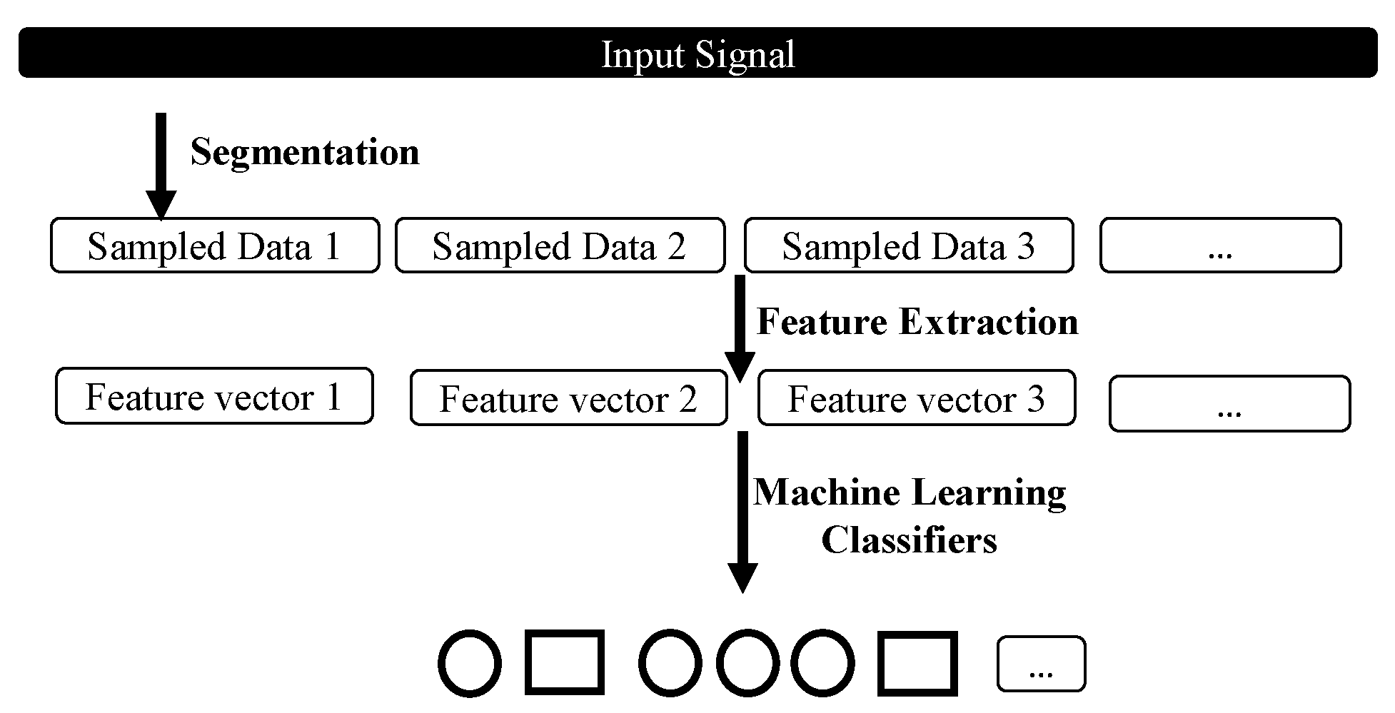
As shown in Figure 2, the standard process of machine-learning-based fall detection consists of three main steps. Acquired sensor signals are firstly segmented into small data blocks and then features that can reflect characteristics of human falls are extracted and fed into classifiers for recognition. According to this process, the rest of this paper is organized as follows. The dataset, signal pre-processing methods and classification protocol used in this work are first explained in Section 2. Section 3 provides a brief introduction on classifiers used. Then, experimental results are presented in Section 4. Finally, Section 5 draws conclusions.

2. Datase and Pre-Processing

2.1. Dataset Description

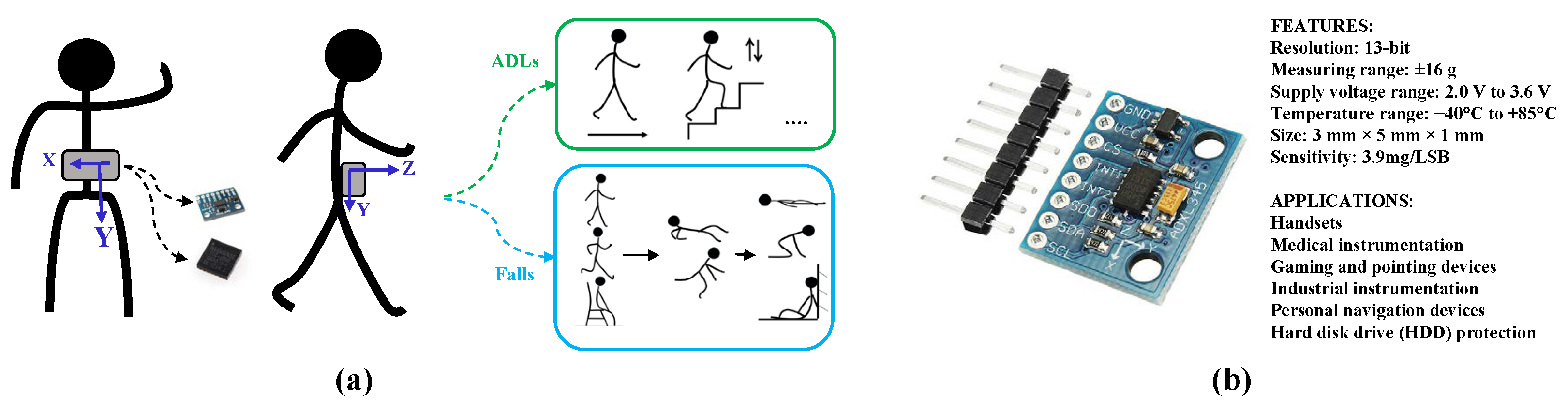
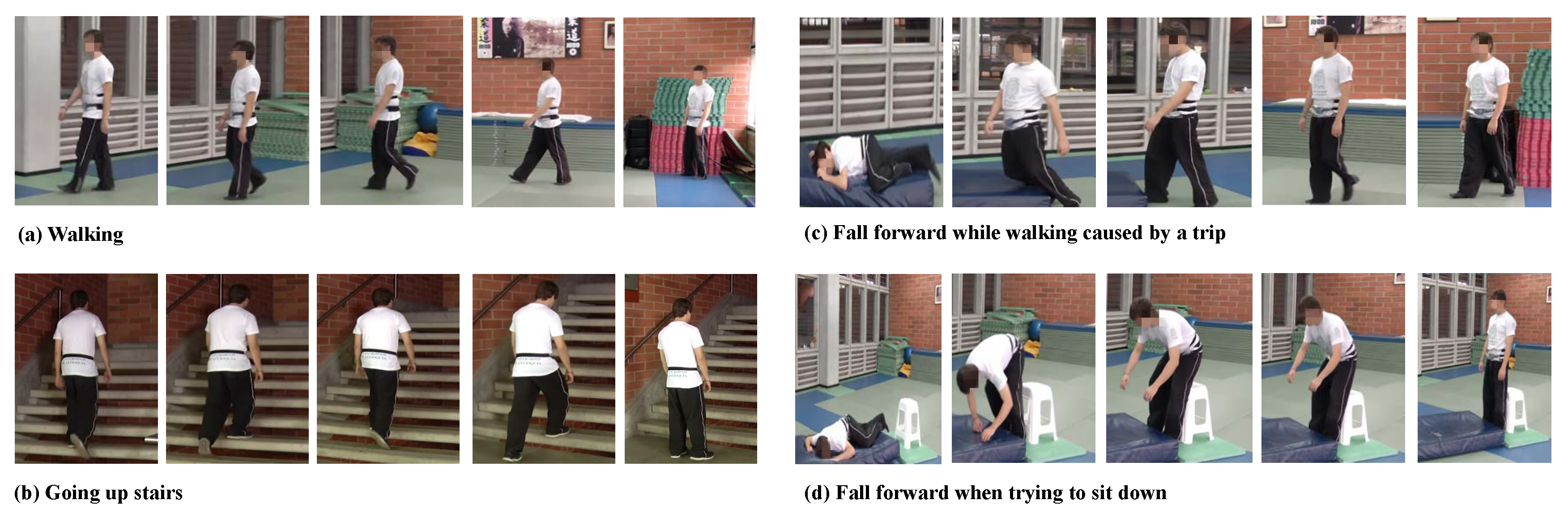
To guarantee a reliable evaluation, a large public dataset known as the SisFall dataset is used in this work [25]. This dataset has been used in previous work for its diversity and integrity [26]. The dataset was recorded with a self-developed embedded device composed of a Kinets MKL25Z128VLK4 microcontroller (NPX, Austin, TX, USA), an Analog Devices (Norwood, MA, USA) ADXL345 accelerometer, a Freescale MMA8451Q accelerometer, an ITG3200 gyroscope, and a 1000 mA/h generic battery. During data collection, the device was tethered on the waist of subjects as shown in Figure 3a with a sampling rate of 200 Hz and then different activities listed in

Table 1. Activities covered in the SisFall dataset.

Code	ADLs	Duration
D01 D02 D03 D04 D05 D06 D07 D08 D09 D10 D11 D12 D13 D14 D15 D16 D17 D18 D19	Walking slowly Walking quickly Jogging slowly Jogging quickly Walking upstairs and downstairs slowly Walking upstairs and downstairs quickly Slowly sit in a half height chair, wait a moment, and up slowly Quickly sit in a half height chair, wait a moment, and up quickly Slowly sit in a low height chair, wait a moment, and up slowly Quickly sit in a low height chair, wait a moment, and up quickly Sitting a moment, trying to get up, and collapse into a chair Sitting a moment, lying slowly, wait a moment, and sit again Sitting a moment, lying quickly, wait a moment, and sit again Being on one’s back change to lateral position, wait a moment, and change to one’s back Standing, slowly bending at knees, and getting up Standing, slowly bending without bending knees, and getting up Standing, get into a car, remain seated and get out of the car Stumble while walking Gently jump without falling (trying to reach a high object)	100 s 100 s 100 s 100 s 25 s 25 s 12 s 12 s 12 s 12 s 12 s 12 s 12 s 12 s 12 s 12 s 25 s 12 s 12 s
Code	Falls	Duration
F01 F02 F03 F04 F05 F06 F07 F08 F09 F10 F11 F12 F13 F14 F15	Fall-forward while walking caused by a slip Fall-backward while walking caused by a slip Lateral fall while walking caused by a slip Fall-forward while walking caused by a trip Fall-forward while jogging caused by a trip Vertical fall while walking caused by fainting Fall while walking, with use of hands in a table to dampen fall, caused by fainting Fall-forward when trying to get up Lateral fall when trying to get up Fall-forward when trying to sit down Fall-backward when trying to sit down Lateral fall when trying to sit down Fall-forward while sitting, caused by fainting or falling asleep Fall-backward while sitting, caused by fainting or falling asleep Lateral fall while sitting, caused by fainting or falling asleep	15 s 15 s 15 s 15 s 15 s 15 s 15 s 15 s 15 s 15 s 15 s 15 s 15 s 15 s 15 s

were performed in the classrooms and open spaces of a coliseum at the Universidad de Antioquia (Medellín, Colombia). Some of the data collection scenarios are shown in Figure 4. In order to guarantee safety conditions, falls were simulated using safety landing mats [25]. To collect the dataset, overall 38 volunteers including 15 elder people and 23 young people were employed and the characteristics of these subjects such as sex, age, height, and weight are summarized in

Table 2. Age, height and weight of the subjects.

	Sex	Age	Height (m)	Weight (kg)
Elderly	Female	62–75	1.50–1.69	50–72
	Male	60–71	1.63–1.71	56–102
Adult	Female	19–30	1.49–1.69	42–63
	Male	19–30	1.65–1.83	58–81

.

In this work, only acceleration data acquired from the three-axial accelerometer ADXL345 are used as in [25]. As shown in Figure 3b, the ADXL345 is an energy-efficient accelerometer that has been widely embedded in handsets, medical instrumentation, gaming, and pointing devices, industrial instrumentation, and personal navigation devices. The ADXL345 used is configured with a measuring range of ±16 g and a resolution of 13 bits with a sensitivity of 3.9 mg/LSB. The supply voltage range of ADXL345 is 2.0 V to 3.6 V and the temperature range is −40 ${}^{\circ }$C to +85 ${}^{\circ }$C. Moreover, the accelerometer has a small size of 3 mm × 5 mm × 1 mm [27].

Since it has been found that there is no significant gain for having sampling frequency higher than 25 Hz in fall detection [26], the original acceleration measurements are first downsampled to 25 Hz. In data downsampling, original acceleration measurements are decimated by an integer factor instead of resampling sensing data, where artifacts and distortion may occur. When the original sensing data $S=\left\{s_1,s_2,\dots ,s_l\right\}$ is downsampled by an integer of n, it would keep the first sample from every n samples and starting with an integer offset of m as follows.

$$D{S}_m^n=\left\{s_k|k=1+m+\alpha \times n\right\},$$

(1)

where $0\le m<n$, $D{S}_m^n$ is the downsampled data, $\alpha$ is an integer and $0\le \alpha \le \lfloor \frac{l}{n}\rfloor$. If the original sampling rate is R Hz, the sensor data after downsampling is $\frac{R}{n}$ Hz. In this work, an integer of eight is used to downsample sensor signals to 25 Hz.

2.2. Data Pre-Processing

In this section, the segmentation, feature extraction and data oversampling methods used to pre-process the acquired acceleration measurements are explained in detail.

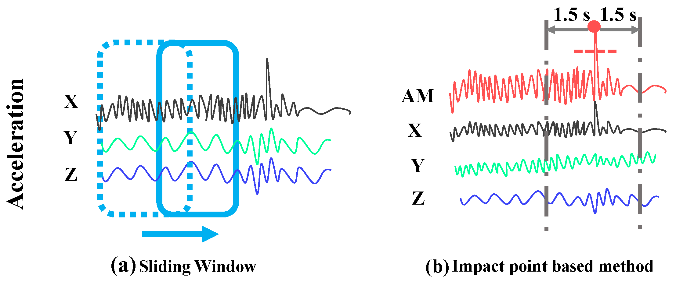
2.2.1. Data Segmentation with Impact Point

To segment sensor signals for classification, most researchers in literature used a sliding window method shown in Figure 5a, where sensor data are continuously segmented by a moving window with an overlap. This method is simple but energy-intensive since the classifiers need to operate continuously at a small interval. Moreover, it is also not accurate in extracting data blocks of falls since a sliding window with an overlap may not locate exactly on the whole data block of a fall. The window may only cover a part of the fall and another part of human activities happened before the fall such as walking or running and this may cause bias in recognition.

To deal with this, an impact point-based data segmentation method is used in this work. It is based on the fact that a fall is always associated with an extreme impact between the human body and the ground. By detecting the impact, the sensor signals of falls can be accurately located. Moreover, a large number of uninterested sensor data (e.g., data of activities without evident impact such as sitting, standing or lying) can be excluded to avoid unnecessary recognition and save energy.

To detect the impact point, the acceleration magnitude (AM) that can reflect the energy contained in the sensor signals is used with a threshold of 1.6 g according to [28,29]. The AM can be obtained as following:

$$AM\left(a\left[n\right]\right)=\sqrt{a{\left[n\right]}_x^2+a{\left[n\right]}_y^2+a{\left[n\right]}_z^2},$$

(2)

where a represents the acceleration measurements on different axes of the accelerometer.

Figure 5b shows the process of data segmentation with an impact point in fall detection. Once an impact is identified with the pre-defined threshold of AM, a window is centered on the impact point to extract the complete fall process. In the experiment, a window of 3 s is used according to previous work [18].

2.2.2. Feature Extraction

Once sensor signals are segmented, meaningful features should be extracted for classification. As for neural networks, features can be extracted automatically. However, human-design features that can reflect the shape, energy, and dispersion of sensor signals are needed for other conventional machine learning classifiers such as SVM and KNN. In this work, 13 types of statistical features that have been used in literature [26] are extracted from acceleration measurements on each axis:

(1)

Minimum values of acceleration measurements;

(2)

Maximum values of acceleration measurements;

(3)

Mean values of acceleration measurements;

(4)

Median values of acceleration measurements;

(5)

Interquartile range of acceleration measurements;

(6)

Variance of acceleration measurements;

(7)

Standard deviation of acceleration measurements;

(8)

Mean absolute deviation of acceleration measurements;

(9)

Root mean square of acceleration measurements;

(10)

Entropy of acceleration measurements;

(11)

Energy of acceleration measurements;

(12)

Skewness of acceleration measurements;

(13)

Kurtosis of acceleration measurements.

2.2.3. Mitigating Effects of Class Imbalance

One issue with dataset generation that is frequently overlooked in previous work is class imbalance. It is quite common in fall detection datasets, due to the difficulty of collecting fall trials and practical constraints on collecting data from multiple subjects, that the number of data samples for each class are not equal. Imbalance in the dataset can cause algorithms to be biased toward the classes having more data. The data imbalance in the Sisfall dataset is larger than 50:1 (ADLs to falls).

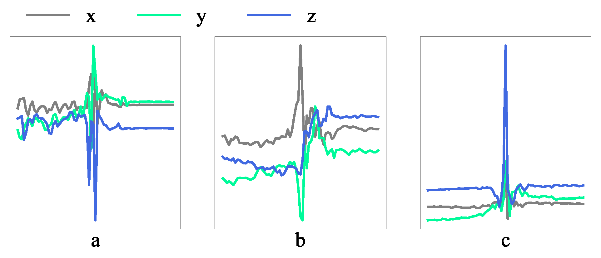
To deal with this, the synthetic minority oversampling technique (SMOTE) is used on the training dataset to prevent imbalanced learning and avoid overfitting. SMOTE solves the data imbalanced problem by oversampling the samples in the minority class. In oversampling, new instances of minority class are interpolated using the KNN within the feature space. A new synthetic data instance X is generated as follows:

$$X=X_i+rand(0,1)\times (X_j-X_i),$$

(3)

where $X_i$ is a sample of minority class, $X_j$ is one of the nearest neighbors of $X_i$ of the same class. This interpolation process is then repeated for the other nearest neighbors of $X_i$. As a result, SMOTE generates more general regions from the minority class and many machine learning classifiers are able to use the data set for better generalizations. Figure 6 shows some fall trails generated by the SMOTE method in data oversampling.

2.2.4. Evaluation Metrics

In this work, the performance of different classifiers is presented with the confusion matrix, accuracy (ACC), sensitivity (SEN) and specificity (SPE).

Table 3. Overview of a confusion matrix.

Confusion Matrix		Predicted Class
		Falls	ADLs
Actual Class	Falls (P)	TP	FN
	ADLs (N)	FP	TN

shows the confusion matrix in fall detection. In the matrix, true-positive (TP) is the number of observations that are falls and were predicted to be falls, false-negative (FN) is the number of observations that are ADLs but were predicted to be falls, true-negative (TN) is the number of observations that are ADLs and were predicted to be ADLs, and false-positive (FP) is the number of observations that are ADLs but were predicted to be falls (false alarms). P is the number of falls, and N is the number of ADLs observations.

Based on the confusion matrix, ACC, SEN, and SPE are defined as follows:

$$ACC=\frac{TP+TN}{TP+TN+FP+FN}$$

(4)

$$SEN=\frac{TP}{TP+FN}$$

(5)

$$SPE={\displaystyle \frac{TN}{TN+FP}}$$

(6)

In these metrics, ACC is a measure of the overall performance of a classifier. SEN can be used to know how correct a classifier is and SPE can be used to assess the capability of a classifier to avoid misclassifying. Since an accurate classifier with a large number of false alarms is still not acceptable in daily use, both of the abilities to recognize falls and exclude false alarms of classifiers are important. Generally, a classifier is deemed to have a higher level performance only when its accuracy, specificity, and sensitivity are all higher than others.

2.2.5. Classification Protocol

In order to present the performance of different machine learning methods in a realistic way. The SisFall dataset is divided into two parts: the first one contains the activities performed by young adults Y1, …, Y12 and elderly E1, …, E8, while the second part contains activities performed by the remaining young adults Y13, …, Y23 and elderly E9, …, E15. Then, a two-fold cross-validation strategy is conducted on these two different datasets. In this way, activities performed by some subjects are always tested with classifiers trained on different persons, which guarantees realistic evaluation. Finally, the total numbers of TP, TN, FP, and FN are counted from the validation results and used to assess the performance.

3. Machine Learning Methods

In this section, the background of machine learning classifiers used in this paper is introduced to facilitate understanding. Overall eight machine learning approaches are used including four types of conventional methods and four types of neural networks.

3.1. Conventional Machine Learning Methods

Conventional machine learning methods used in this work include SVM, decision tree (DT), KNN, and extreme gradient boosting method (XGB).

3.1.1. SVM

The SVM theory was proposed by Vapnik and Chervonenkis [30] and it has been proven very effective in addressing problems including handwritten digit recognition and face detection in images. The principle of SVM is to find a boundary between two hyperplanes that can separate samples of different classes.

Given the training data $X=\left\{X_1,X_2,\dots ,X_N\right\}$ and corresponding label $Y=\{y_1,y_2,\dots y_N,y_i\in [1,-1]\}$, two hyperplanes can be found:

$$w^T{X}_i+b\ge +1,y_i=+1$$

(7)

$$w^T{X}_i+b\le -1,y_i=-1,$$

(8)

where w and b are the parameters that represent hyperplanes. SVM is to find a boundary between these two hyperplanes meanwhile maximizing the distance $d=\frac{2}{\parallel w\parallel }$ between them.

3.1.2. KNN

KNN classifies an unseen feature vector based on the votes of its most similar samples in the training dataset. Generally, a Euclidean distance function is first used to measure the similarity between the target feature vector and training samples:

$$d(X{}_i,X{}_j)=\sqrt{{(x{}_i{}_1-x{}_j{}_1)}^2+\dots +{(x{}_i{}_n-x{}_j{}_n)}^2}$$

(9)

$$R_k^X=\{X\in R^n,d(X,X_i)\le d(X,X_k)\},$$

(10)

where $d(X_i,X_j)$ means the distance between samples $X_i$ and $X_j$, $R_k^X$ is the group of k nearest neighbors of the new feature vector X. Then, the new feature vector is assigned to the class, to which the majority of its k nearest neighbors belong.

3.1.3. DT

DT solves a classification problem through a series of cascading decision questions. A feature vector, which satisfies a specific set of questions, is assigned to a specific class. This method is represented graphically using a tree structure, where each internal node is a test on a feature compared with the threshold, and the remaining values refer to the decided classes. Its implementation is based on a loop of if/else conditions. Many types of DTs have been generated by different algorithms. In our research, a C4.5 is used.

3.1.4. XGB

The XGB is a meta-algorithm. It is a method that can be used with other machine-learning methods to improve recognition accuracy. It combines the outputs of plenty of “weak” classifiers into a weighted sum that represents the final output. The individual learners can be weak, but as long as the performance of each one is slightly better than random guessing, the final model can be proven to converge to a strong learner. In this paper, XGB embedded with decision trees is used.

In the experiments, the performance of SVM was compared for two different kernels: linear and radial basis function (RBF) kernel, between which the linear kernel was found to yield better results and was finally selected. The parameter searching of k in KNN was performed in a wide range from 1 to 10 and a value of 1 was selected. Model parameters of the XGB were optimized using a grid search over two parameters: the number of trees and maximum depth of the tree. The best results were achieved based on 50 trees with a maximum depth of 3.

3.2. Neural Networks

Neural networks are a family of statistical learning models through replicating the working principle of neurons in the human brain. Overall, four types of neural networks are used in this work including supervised models such as multi-layer perceptron (MLP), convolutional neural network (CNN) and unsupervised autoencoders.

3.2.1. MLP

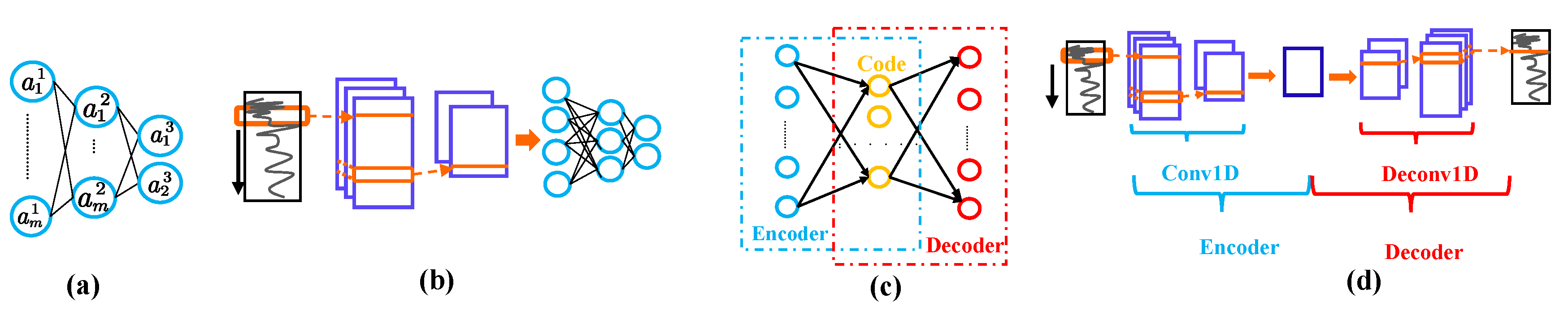
An MLP that is also known as the feed-forward neural network is shown in Figure 7a. It is a model that processes information through a series of interconnected computational neurons. The inputs are fed directly to the outputs via a series of hidden neurons, which are grouped into layers and associated with previous layers using weighted connections. Formally, neurons are defined as the following function:

$$a^{l+1}=\sigma \left(W^l{a}^l+b^l\right),$$

(11)

where $a^l$ is the value of neurons in layer l, ($a_i^l$ denotes the value of neuron i in layer l), W is the weight matrix between layer l and $l+1$, $b^l$ is the bias associated with neurons in layer l and $\sigma$ is the activation function. For the first layer in the network, the neuron value is $a^{\left(1\right)}=x$, which is the input to the neural network (flattened sensor signal in this work). MLPs use a fully-connected topology, where each neuron in the present layer is connected with every neuron in the previous one.

3.2.2. CNN

The architecture of the CNN is shown in Figure 7b. Different from the MLP, there are many additional convolutional layers between the input and fully connected layers. These convolutional layers can help to extract more meaningful feature maps for recognition by conducting convolutional operation on the input signals with different kernels. In the convolutional operation, kernels act as different filters or feature detectors. Formally, a feature map is generated by a kernel as following:

$$a_j^{l+1}\left(\gamma \right)=\sigma \left(b_j^l+\sum _{f=1}^n{k}_{jf}^l\left(\gamma \right)\ast a_f^l\left(\gamma \right)\right),$$

(12)

where $a_j^{l+1}$ means the value of feature map j in layer $l+1$, $\sigma$ is the activation function, n is the number of feature maps in layer l, $k_{jf}^l$ denotes the kernel that convolves over feature maps in layer l to create the feature map j in layer $l+1$, $a^l$ is the value of feature maps in layer l, $b^l$ is the bias vector. Once feature maps are generated with convolutional layers, they will be flattened and fed into subsequent fully-connected layers for classification.

The training of MLP and CNN is based on optimizing their parameters including weights and biases and the optimization can be realized by minimizing the following cross-entropy error function:

$$J\left(w,b\right)=-\frac{1}{N}\sum _{n=1}^N\left[y_{n}log{\overline{y}}_n+\left(1-y_n\right)log\left(1-{\overline{y}}_n\right)\right],$$

(13)

where, w and b denote the weight and bias parameters, N means the number of samples, $y_n$ is the real value of the sample n and ${\overline{y}}_n$ is the prediction from neural networks. Given the training dataset $X=\left\{X_1,X_2,\dots ,X_N\right\}$ and corresponding label $Y=\{y_1,y_2,\dots y_N,y_i\in [1,0]\}$, the optimal values of parameters in MLP and CNN can be found based on gradient-descent approach.

3.2.3. Autoencoders

Autoencoders are neural networks that are trained in an unsupervised way. Autoencoders aim to learn the representation (encoding) of sensor signals with the purpose to reconstruct themselves. Since only sensor signals of different activities without labels are needed during training, autoencoders are known as the unsupervised models. Figure 7c shows a dense autoencoder (DAE) that is built based on an MLP. The MLP is used as an encoder $\delta$ in the DAE with another MLP that has a symmetrical structure as a decoder $\psi$. Similarly, a convolutional autoencoder (CAE) can be built based a CNN as shown in Figure 7d.

The aims of encoders and decoders in autoencoders are to learn how to condense input signals into representative features and then use them to reconstruct the signal as follows:

$$\delta :h_w{\left(x\right)}^{\delta }\to c$$

(14)

$$\psi :h_w^{\psi }\left(c\right)\to x^{{}^{\prime }},$$

(15)

where, x means the input signal, c means the condensed code and $x^{{}^{\prime }}$ means the reconstructed signal.

Different from MLP and CNN, the training of DAE and CAE is based on minimizing the construction error between the original and reconstructed signals and a mean square error function is used during training:

$$\delta ,\psi =argmin\left|\right|x-x^{{}^{\prime }}{\left|\right|}^2=argmin\left|\right|x-h_w^{\psi }\left(h_w{\left(x\right)}^{\delta }\left(x\right)\right){\left|\right|}^2.$$

(16)

In this work, the DAE and CAE are built based on the MLP and CNN used. After unsupervised training, the encoders in DAE and CAE are extracted out and concatenated with a fine-turned fully connected layer for recognition.

3.2.4. Neural Network Architectures

Overall, seven neural networks are evaluated in this paper. Three of them are the models that have achieved superior performance in literature. They are used as the baselines to compare with the lightweight neural networks proposed in this paper:

• (CNN-HE) [23]: CNN-HE consists of two convolutional layers (each appended with a max-pooling layer) and two fully-connected layers. The first convolutional layer consists of 32 kernels and the second layer consists of 64 kernels. The size of kernels used is 1 × 5 with a stride of 1. Furthermore, the first fully-connected layer consists of 512 neurons and the second layer consists of 8 neurons (change to 1 in this work) for classification.
• (CNN-3B3Conv) [24]: CNN-3B3Conv consists of three-layer blocks. The first block consists of three convolutional layers and one max-pooling layer. Each of the convolutional layer consists of 64 kernels with a size of 1 × 4. The second block also consists of three convolutional layers and one max-pooling layer, but the kernel size is set to 1 × 3 empirically. The third block consists of three fully-connected layers with 64 neurons, 32 neurons and two neurons (changed to one in this work) respectively.
• CNN-EDU [22]: CNN-EDU consists of four convolutional layers composed by 16 kenerls, 32 kenerls, 64 kenerls and 128 kenerls ($1\times 5$) respectively. Each convolutional layer is also appended with a pooling layer. Moreover, two fully-connected layers are appended in the end.

Another four neural networks are the lightweight neural networks used in this work. They are designed based on the evaluation results in

Table 4. Evaluation of different CNN architectures.

Filter Size	Depth	Width	Acc.(%)	Filter Size	Depth	Width	Acc.(%)	Filter Size	Depth	Width	Acc.(%)
1 × 2	1	5	99.85%	1 × 5	1	5	99.89%	1 × 10	1	5	99.89%
	1	10	99.90%		1	10	99.94%		1	10	99.91%
	1	30	99.91%		1	30	99.94%		1	30	99.94%
	2	5	99.77%		2	5	99.83%		2	5	99.91%
	2	10	99.91%		2	10	99.93%		2	10	99.92%
	2	30	99.93%		2	30	99.94%		2	30	99.94%
	3	5	99.88%		3	5	99.91%		3	5	99.91%
	3	10	99.89%		3	10	99.93%		3	10	99.92%
	3	30	99.89%		3	30	99.94%		3	30	99.94%

and

Table 5. Evaluation of different MLP architectures.

Depth	Width	Acc.(%)	Depth	Width	Acc.(%)
1	16	99.91%	2	16	99.90%
1	32	99.91%	2	32	99.91%
1	64	99.92%	2	64	99.91%
3	16	99.90%	4	16	99.88%
3	32	99.91%	4	32	99.92%
3	64	99.90%	4	64	99.92%

. In Table 4, we compare the effect of filter size, as well as the depth (layer number) and width (kernel number) of the CNN on the resulting accuracy. Notably, the max-pooling layers and the additional fully-connected layers, which were often appended after convolutional layers in previous work, are abandoned due to information loss [31] and parameter redundancy.

Based on Table 4, a simple CNN consisting of a single convolutional layer composed of ten 1 × 5 kernels with a stride of 3, and one fully-connected layer is chosen (as highlighted in bold in Table 2). Similarly, a simple MLP consisting of a single hidden layer with 64 hidden neurons is selected according to the results in Table 5. Meanwhile, a DAE and a CAE are built based on the lightweight MLP and CNN selected.

In all of these neural networks, the rectified linear units (ReLU) is used as the activation function except in the last fully-connected layers where a sigmoid function is used for classification. Moreover, a learning rate of 0.001 and a batch size of 128 are proved the best and used with the ADAM algorithm [32] in parameter optimizing.

4. Experiment Results and Discussion

4.1. Lightweight Neural Networks against Conventional Methods

To guarantee reliable experimental results, each of the classifiers used was run for 10 rounds (detailed results see Appendix A), and the final average results are used for evaluation. Firstly, the performance of lightweight neural networks are compared with conventional machine learning methods in

Table 6. Average detection results of lightweight neural networks against conventional machine learning methods.

Classifiers →	Conventional Methods				Leight Weight Neural Networks
Metrics ↓	XGB	KNN	SVM	DT	MLP	DAE	CAE	CNN
SEN.(%)	99.32	90.91	98.27	97.77	98.31	99.07	99.20	98.71
SPE.(%)	99.36	98.70	98.30	98.96	99.96	99.83	99.93	99.96
ACC.(%)	99.35	98.52	98.30	98.93	99.92	99.81	99.91	99.94
TP	1777.8	1627.4	1759	1750.1	1759.7	1773.4	1775.6	1767.1
FN	12.2	162.6	31	39.9	30.3	16.6	14.4	22.9
FP	496.7	1000.9	1309.4	799.4	33.3	131.1	57.9	26.9
TN	76,428.3	75,924.1	75,615.6	76,125.6	76,891.7	76,793.9	76,867.1	76,898.1

.

As we can see from the results, the XGB performs the best with an accuracy of 99.35% among conventional methods. DT and KNN come next to XGB with an accuracy of 98.93% and 98.52%. The SVM performs the worst with an accuracy of 98.30%. The improvement of the boosting method over other conventional classifiers is evident, especially on the false positive samples (decrease 1309.4 of SVM, 1000.9 of KNN and 799.4 of DC to 496.7 of XGB).

As for the lightweight neural networks, much better results can be obtained. The accuracy of each neural network was higher than 99.5% which was even higher than the best conventional method (99.35% of XGB). The best results of neural networks were obtained from the CNN with an accuracy of 99.94%, a sensitivity of 98.71% and a specificity of 99.96%. These metrics show significant improvement over conventional methods, especially on decreasing false alarms. Let us consider, as an example, the specificity of CNN and XGB which shows a specificity of 99.36%. Now, comparing this result with that of CNN i.e., 99.96%, the latter improved the specificity only by 0.59%. However, this difference is significant as it means reducing the number of false alarms from 497.7 to 26.9 only.

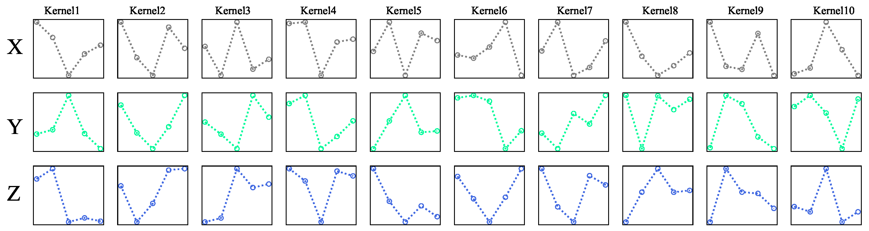
In our analysis, the better results of CNN were partly due to its advanced modeling ability, but mainly due to the ability of CNN to extract local features. The convolutional kernels in the CNN are visualized in Figure 8, where X, Y, and Z denote the kernels on each axis of acceleration measurements. As we can see, these kernels were in different patterns and shapes and were also different on every axis. Some of them were line segments with a big slope and some of them are line segments fluctuating uniformly. These kernels act as various pattern detectors and move along the input signals to identify certain signal patterns on different locations for classification. Compared to other methods that depend on features extracted from the whole data segments, these automatically learned kernels can help CNN to extract local features that can reveal the differences between signals of falls and ADLs on a much smaller scale. In this work, kernels in the CNN can extract local features on a scale as small as 0.2 s (1 × 5) at each step for recognition.

On the other hand, although autoencoders have been proved effective in learning the intrinsic characteristics of data, their slightly poor performance over supervised neural networks proves the efficacy of autoencoders is not evident in fall detection. This may due to the fact that sensor signals used in fall detection are usually not complex that only last for many seconds. Hence, supervised models are enough to learn effective features for recognition.

4.2. Leightweight Neural Networks against Baseline Models

The performance of lightweight neural networks is compared with baseline models used in previous work in

Table 7. Average detection results of lightweight neural networks against baseline models.

Classifiers →	Baseline Models			Leight Weight Neural Networks
Metrics ↓	CNN-HE	CNN-3B3	CNN-EDU	MLP	DAE	CAE	CNN
SEN.(%)	99.23	99.45	99.51	98.31	99.07	99.20	98.71
SPE.(%)	99.94	99.93	99.93	99.96	99.83	99.93	99.96
ACC.(%)	99.93	99.92	99.93	99.92	99.81	99.91	99.94
TP	1776.2	1780.2	1781.3	1759.7	1773.4	1775.6	1767.1
FN	13.8	9.8	8.7	30.3	16.6	14.4	22.9
FP	45.8	52.2	51.8	33.3	131.1	57.9	26.9
TN	76,879.2	76,872.8	76,873.2	76,891.7	76,793.9	76,867.1	76,898.1
PARA	$\mathbf{60.1}\times {\mathbf{10}}^{\mathbf{4}}$	$10.6\times {10}^4$	$\mathbf{8}.\mathbf{7}\times {\mathbf{10}}^{\mathbf{4}}$	$1.5\times {10}^4$	$1.5\times {10}^4$	411	411
FLOPs	2 M	6.9 M	1.4 M	0.03 M	0.03 M	0.008 M	0.008 M

. Notably, to further compare the complexity of different neural networks, the number of parameters (PARA) and the number of floating-point operations (FLOPs [33], detailed calculation see Appendix B) of each neural network are also listed in Table 7.

As we can see from the accuracy metrics, even though the baseline models are much deeper and more complex, they could only achieve a similar accuracy around 99.93% as the lightweight models. However, the number of parameters of baseline models are generally hundreds of times the lightweight models, which also means hundreds of times the storage requirement. The simplest models are the lightweight CNN and CAE with only 411 parameters and the most complex one is CNN-HE with $60.1\times {10}^4$ parameters.

Furthermore, the complex structure of baseline models also leads to more computational cost during classification. In the baseline models, even the simplest mode (CNN-EDU) still requires 1.4 MFLOPs to make one decision (fall/no fall), which is hundreds of times the lightweight CNN and CAE. Such large FLOPs mean higher power requirements and more frequent battery recharging that make the wearable fall detector more obtrusive to use in daily life.

Even though many deep neural networks that consist of more than three layers with thousands of neurons have been the focus in previous work, the experiment results prove that lightweight neural networks which consist of only one hidden layer with less than 100 neurons are enough to achieve satisfying accuracy in fall detection. These lightweight neural networks have fewer parameters and smaller FLOPs that make them more suitable to be embedded in wearable devices that usually have real-time requirements restricting the memory size and computation power. In this work, the most simple and accurate neural network is the lightweight CNN used, which has only 411 parameters (160 from the convolutional layer and 251 from the final fully-connected layer). The total storage space needed is only 4 ×$\delta$ = 1.2 KB (using 4-Byte floating-point numbers)and the FLOPs needed in classification is 0.008 MFLOPs that is only a few hundredth of deep models used previously.

5. Conclusions

As the population of elderly people is increasing fast, providing healthcare service to the elderly to reduce living risks associated with their daily life is increasingly demanded. Falls are one of the main threats to the life of elder people that have caused a large number of accidents. The treatment of falls has also been a huge financial burden to society. Since early detection of falls can prevent the extremely fatal long lying time, the quest to detect falls of elder people with the highest possible accuracy using wearable sensors has been a hot research topic in past decades.

Even though a large number of work has been done, developing highly accurate embeddable models with lightweight architectures and feasible computational cost is still an obstacle to realize a pervasive sensing fall detector using wearable devices. In this paper, different types of lightweight neural networks are proposed including supervised and unsupervised models. Experiment results prove the superior performance of proposed lightweight neural networks. The best results are obtained from a lightweight CNN. This model can provide an accuracy beyond 99.9% with a small size of only 1.2 KB and a low computational cost of 0.008 MFLOPs that is more suitable to be implemented on wearable devices.

In the future, we plan to design different types of neural networks to detect human falls using other wearable devices such as the smartphone to provide the fall detection service to the general public. We also plan to improve our model to detect other human activities such as walking, running and jumping to realize a cognitive wearable module to use in healthcare industry.

References

- United Nations, Department of Economic and Social Affairs. World Population Prospects: The 2017 Revision, Key Findings and Advance Tables. ESA/P/WP/248. 2017. Available online: https://population.un.org/wpp/Publications/ (accessed on 6 November 2019).
- Murray, C.J.; Lopez, A.D. The global burden of disease: A comprehensive assessment of mortality and disability from diseases, injuries, and risk factors in 1990 and projected to 2020: summary. Glob. Burd. Dis. Inj. Ser. 1996, 1, 201–246. [Google Scholar]
- Schwendimann, R. Patient falls: A Key Issue in Patient Safety in Hospitals. Ph.D. Thesis, University of Basel, Basel, Switzerland, 2006. [Google Scholar]
- Schwickert, L.; Becker, C.; Lindemann, U.; Maréchal, C.; Bourke, A.; Chiari, L.; Helbostad, J.; Zijlstra, W.; Aminian, K.; Todd, C.; et al. Fall detection with body-worn sensors. Z. Für Gerontol. Geriatr. 2013, 46, 706–719. [Google Scholar] [CrossRef] [PubMed]
- Büsching, F.; Post, H.; Gietzelt, M.; Wolf, L. Fall detection on the road. In Proceedings of the 2013 IEEE 15th International Conference on e-Health Networking, Applications and Services (Healthcom 2013), Lisbon, Portugal, 9–12 October 2013; pp. 439–443. [Google Scholar]
- Aguiar, B.; Rocha, T.; Silva, J.; Sousa, I. Accelerometer-based fall detection for smartphones. In Proceedings of the 2014 IEEE International Symposium on Medical Measurements and Applications (MeMeA), Lisboa, Portugal, 11–12 June 2014; pp. 1–6. [Google Scholar]
- Hakim, A.; Huq, M.S.; Shanta, S.; Ibrahim, B. Smartphone based data mining for fall detection: Analysis and design. Procedia Comput. Sci. 2017, 105, 46–51. [Google Scholar] [CrossRef]
- Rougier, C.; Meunier, J.; St-Arnaud, A.; Rousseau, J. Robust Video Surveillance for Fall Detection Based on Human Shape Deformation. IEEE Trans. Circuits Syst. Video Technol. 2011, 21, 611–622. [Google Scholar] [CrossRef]
- Cucchiara, R.; Prati, A.; Vezzani, R. A multi-camera vision system for fall detection and alarm generation. Expert Syst. 2007, 24, 334–345. [Google Scholar] [CrossRef]
- Mohamed, O.; Choi, H.; Iraqi, Y. Fall Detection Systems for Elderly Care: A Survey. In Proceedings of the 2014 6th International Conference on New Technologies, Mobility and Security (NTMS), Dubai, United Arab Emirates, 30 March–2 April 2014; pp. 1–4. [Google Scholar]
- Zhang, Z.; Conly, C.; Athitsos, V. A Survey on Vision-based Fall Detection. In Proceedings of the 8th ACM International Conference on PErvasive Technologies Related to Assistive Environments, Corfu, Greece, 1–3 July 2015; pp. 46:1–46:7. [Google Scholar]
- Kamilaris, A.; Pitsillides, A. Mobile Phone Computing and the Internet of Things: A Survey. IEEE Internet Things J. 2016, 3, 885–898. [Google Scholar] [CrossRef]
- Zhang, Y.; Sun, L.; Song, H.; Cao, X. Ubiquitous WSN for Healthcare: Recent Advances and Future Prospects. IEEE Internet Things J. 2014, 1, 311–318. [Google Scholar] [CrossRef]
- Sezer, O.B.; Dogdu, E.; Ozbayoglu, A.M. Context-Aware Computing, Learning, and Big Data in Internet of Things: A Survey. IEEE Internet Things J. 2018, 5, 1–27. [Google Scholar] [CrossRef]
- Chen, M.; Li, Y.; Luo, X.; Wang, W.; Wang, L.; Zhao, W. A Novel Human Activity Recognition Scheme for Smart Health Using Multilayer Extreme Learning Machine. IEEE Internet Things J. 2019, 6, 1410–1418. [Google Scholar] [CrossRef]
- De Quadros, T.; Lazzaretti, A.E.; Schneider, F.K. A Movement Decomposition and Machine Learning-Based Fall Detection System Using Wrist Wearable Device. IEEE Sens. J. 2018, 18, 5082–5089. [Google Scholar] [CrossRef]
- Liu, Z.; Cao, Y.; Cui, L.; Song, J.; Zhao, G. A benchmark database and baseline evaluation for fall detection based on wearable sensors for the internet of medical things platform. IEEE Access 2018, 6, 51286–51296. [Google Scholar] [CrossRef]
- Aziz, O.; Musngi, M.; Park, E.J.; Mori, G.; Robinovitch, S.N. A comparison of accuracy of fall detection algorithms (threshold-based vs. machine learning) using waist-mounted tri-axial accelerometer signals from a comprehensive set of falls and non-fall trials. Med. Biol. Eng. Comput. 2017, 55, 45–55. [Google Scholar] [CrossRef] [PubMed]
- Wang, J.; Chen, Y.; Hao, S.; Peng, X.; Hu, L. Deep learning for sensor-based activity recognition: A survey. Pattern Recognit. Lett. 2019, 119, 3–11. [Google Scholar] [CrossRef]
- Theodoridis, T.; Solachidis, V.; Vretos, N.; Daras, P. Human fall detection from acceleration measurements using a Recurrent Neural Network. In Precision Medicine Powered by pHealth and Connected Health; Springer: Heidelberg, Germany, 2018; pp. 145–149. [Google Scholar]
- Mauldin, T.; Canby, M.; Metsis, V.; Ngu, A.; Rivera, C. SmartFall: A smartwatch-based fall detection system using deep learning. Sensors 2018, 18, 3363. [Google Scholar] [CrossRef] [PubMed]
- Casilari, E.; Lora-Rivera, R.; García-Lagos, F. A Wearable Fall Detection System Using Deep Learning. In International Conference on Industrial, Engineering and Other Applications of Applied Intelligent Systems; Springer: Heidelberg, Germany, 2019; pp. 445–456. [Google Scholar]
- He, J.; Zhang, Z.; Wang, X.; Yang, S. A Low Power Fall Sensing Technology Based on FD-CNN. IEEE Sens. J. 2019, 19, 5110–5118. [Google Scholar] [CrossRef]
- Santos, G.L.; Endo, P.T.; Monteiro, K.H.d.C.; Rocha, E.d.S.; Silva, I.; Lynn, T. Accelerometer-Based Human Fall Detection Using Convolutional Neural Networks. Sensors 2019, 19, 1644. [Google Scholar] [CrossRef] [PubMed]
- Sucerquia, A.; López, J.; Vargas-Bonilla, J. SisFall: A fall and movement dataset. Sensors 2017, 17, 198. [Google Scholar] [CrossRef]
- Liu, K.; Hsieh, C.; Hsu, S.J.; Chan, C. Impact of Sampling Rate on Wearable-Based Fall Detection Systems Based on Machine Learning Models. IEEE Sens. J. 2018, 18, 9882–9890. [Google Scholar] [CrossRef]
- Devices, A. ADXL345 Datasheet; Analog Devices: Norwood, MA, USA, 2010. [Google Scholar]
- Karantonis, D.M.; Narayanan, M.R.; Mathie, M.; Lovell, N.H.; Celler, B.G. Implementation of a real-time human movement classifier using a triaxial accelerometer for ambulatory monitoring. IEEE Trans. Inf. Technol. Biomed. 2006, 10, 156–167. [Google Scholar] [CrossRef]
- Kau, L.; Chen, C. A Smart Phone-Based Pocket Fall Accident Detection, Positioning, and Rescue System. IEEE J. Biomed. Health Inform. 2015, 19, 44–56. [Google Scholar] [CrossRef]
- Cortes, C.; Vapnik, V. Support-vector networks. Mach. Learn. 1995, 20, 273–297. [Google Scholar] [CrossRef]
- Ronao, C.A.; Cho, S.B. Human activity recognition with smartphone sensors using deep learning neural networks. Expert Syst. Appl. 2016, 59, 235–244. [Google Scholar] [CrossRef]
- Kingma, D.P.; Ba, J. Adam: A method for stochastic optimization. arXiv 2014, arXiv:1412.6980. [Google Scholar]
- Molchanov, P.; Tyree, S.; Karras, T.; Aila, T.; Kautz, J. Pruning convolutional neural networks for resource efficient inference. arXiv 2016, arXiv:1611.06440. [Google Scholar]
Figure 1.
The slippery living places in Kelowna (Canada), which are covered with snow and ice in winter.
Figure 2.
Recognition process of machine learning methods.
Figure 3.
Description of the device used in SisFall dataset including (a) the device setting and (b) the accelerometer used in this work.
Figure 4.
Data collection scenarios in the SisFall dataset.
Figure 5.
Different segmentation methods.
Figure 6.
Fall trails generated using the synthetic minority oversampling technique (SMOTE).
Figure 7.
Different types of neural networks. (a) multi-layer perceptron (MLP); (b) convolutional neural network (CNN); (c) dense autoencoder (DAE); (d) convolutional autoencoder (CAE).
Figure 8.
Visulization of convolutional kernels in the CNN.