Deep, Consistent Behavioral Decision Making with Planning Features for Autonomous Vehicles

Abstract

Autonomous driving promises to be the main trend in the future intelligent transportation systems due to its potentiality for energy saving, and traffic and safety improvements. However, traditional autonomous vehicles’ behavioral decisions face consistency issues between behavioral decision and trajectory planning and shows a strong dependence on the human experience. In this paper, we present a planning-feature-based deep behavior decision method (PFBD) for autonomous driving in complex, dynamic traffic. We used a deep reinforcement learning (DRL) learning framework with the twin delayed deep deterministic policy gradient algorithm (TD3) to exploit the optimal policy. We took into account the features of topological routes in the decision making of autonomous vehicles, through which consistency between decision making and path planning layers can be guaranteed. Specifically, the features of a route extracted from path planning space are shared as the input states for the behavioral decision. The actor-network learns a near-optimal policy from the feasible and safe candidate emulated routes. Simulation tests on three typical scenarios have been performed to demonstrate the performance of the learning policy, including the comparison with a traditional rule-based expert algorithm and the comparison with the policy considering partial information of a contour. The results show that the proposed approach can achieve better decisions. Real-time test on an HQ3 (HongQi the third ) autonomous vehicle also validated the effectiveness of PFBD.

1. Introduction

Autonomous driving (AD) has been vastly investigated in different domains for several decades and has a wide variety of applications, especially in intelligent transportation systems. AD provides more economic, comfortable and safer service than human drivers with fewer collision risks. The behavior decision and trajectory planning system is a key component of AD.

Presently, as a mature, rule-based decision and planning method, finite state machines (FSMs) [1,2] have been applied in most autonomous vehicles. Nonetheless, FSMs still have problems with guaranteeing decisions’ accuracy, especially in complex scenarios, due to the difficulty in determining the boundary condition of different states and going through all states with limited experience. To make the vehicles more intelligent and more acceptable for human beings, learning methods have been attractive in recent years to enhance decisions in AD. Among them, neural networks related approaches [3,4,5] have been used to navigate autonomous vehicles due to their strong capacity of mapping inputs to control signals. The raw pixels from cameras [3,4] were used to train neural networks for keeping a vehicle in a lane, which proves that the task of lane following can be learned from the only limited training signal (steering) in a supervised manner. Fusing multiple inputs (LIDAR (light detection and ranging) raw inputs, global direction and GPS), a full convolutional neural network [5] generated driving paths in a more explainable output. In fact, both rule-based and supervised learning based decision policies have the bottleneck of exploring unknown or complex scenarios.

Reinforcement Learning (RL) focuses on finding a balance between exploration and exploitation, and learns optimal policy by interacting with environments. Thus, RL promises to learn more complete decision policy than rule-based or supervised learning based methods. Deep reinforcement learning (DRL), a combination of (RL) and deep learning (DL), has been the hottest topic in the artificial intelligence (AI) discipline. Especially after the win of AI in the game Go [6], DRL has been applied in intelligent transportation systems and automated vehicles.

One class of DRL methods use limited features as inputs, where features are specially selected with experience. Some researchers have used DRL for autonomous vehicles in subsystems, such as energy management systems (EMSs) [7], route planning [8], and behavioral decisions (lane changes, on-ramp merging, etc.) [9,10,11]. Deep Q learning (DQN) [11] was used to learn the lateral control policy with only eight states involving information of vehicles and the road. Aradi et al. [9] used the REINFORCE algorithm to learn the driving policy mapping 16 continuous states as inputs to train the steer and acceleration demand. These methods can hardly be practical, since modeling a vehicle’s lane change behavior with limited information is impossible in real traffic. Wolf et al. [10] explored a compact semantic state model of lane change with more complete information and trained the policy with DQN. Although the model can adapt to a variety of scenarios, the agent collides with other vehicles at high probability.

To learn a simple and explainable driving policy, either states or actions or both in the discrete semantic form were used [11,12,13,14]. States can be "close to the front vehicle" and "far to the front vehicle" and the actions can be overtake, left change, give way and accelerate, respectively. Li et al. [13] used the hierarchical game theory to train a driving policy from low-level to high-level step by step. You et al. [14] used a Q-network to learn discrete optimal actions. For common traffic, an artificial reward function was used. For traffics with little knowledge, the reward function was learned through inverse reinforcement learning (IRL) with the maximum entropy principle.

Some researchers studied the sub-modules of autonomous vehicles, such as longitudinal following and lateral control [15,16,17,18]. Zhu et al. [15] used DDPG [19] to teach a human-like autonomous car-following model, which has high trajectory-reproducing accuracy and generalized-capability. Based on parameterized batch actor-critic learning algorithm, Huang et al. [17] obtained a near-optimal lateral control policy for vehicles. The policy can automatically adjust the fuel/brake signals to track target velocity.

Another class of methods focuses on learning driving policy from raw sensor inputs, such as those from cameras, LIDAR and screen shots of a simulator [3,4,5,20,21,22]. Sallab [20] et al. proposed a new framework of DRL for autonomous vehicles, which combines LSTM and attention networks to capture the spatial features. The framework was tested on the simulation platform TORCS. Chen [22] proposed an end-to-end path planner for autonomous vehicles based on a theory called parallel planning. A deep Q-network was used to strength their motion planner with fewer mistakes. However, the effect of a deep Q-network was not given in their publication.

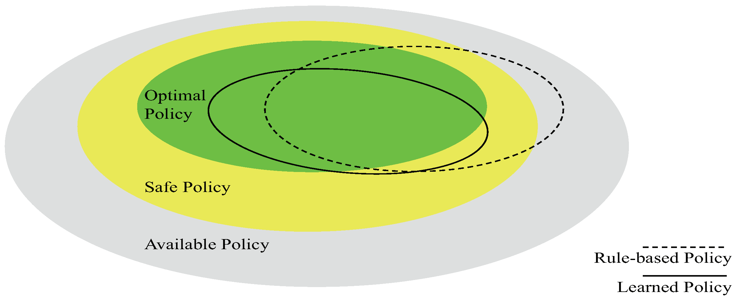
As illustrated in Figure 1, the policy does perform better than experts and traditional decision models do in some situations. However, it can hardly be directly used for behavioral decisions or control in reality. One concern is the transferability of the policy learned by end-to-end methods. The screen shots used as input states differ from raw pixels of real cameras. Besides, the same abstract scenarios, in reality, may have quite abundant images due to different weather, seasons, road conditions, etc. Thus, it is questionable to use a simulator’s policy trained from images. The other concern is the inconsistency between behavioral decision and trajectory planning. In the autonomous driving system, the low-level planner will check whether space is enough to perform a maneuver from the decision level. Taking a left change command from the behavioral decision system, for example, the motion planner, firstly, evaluates whether the gaps are enough for the ego agent to merge in. If space is wide enough, the maneuver is executed with a path generated; otherwise, the command will be ignored for safety’s sake. The final conservative strategy must be a compromise between an optimal policy and a safe one.

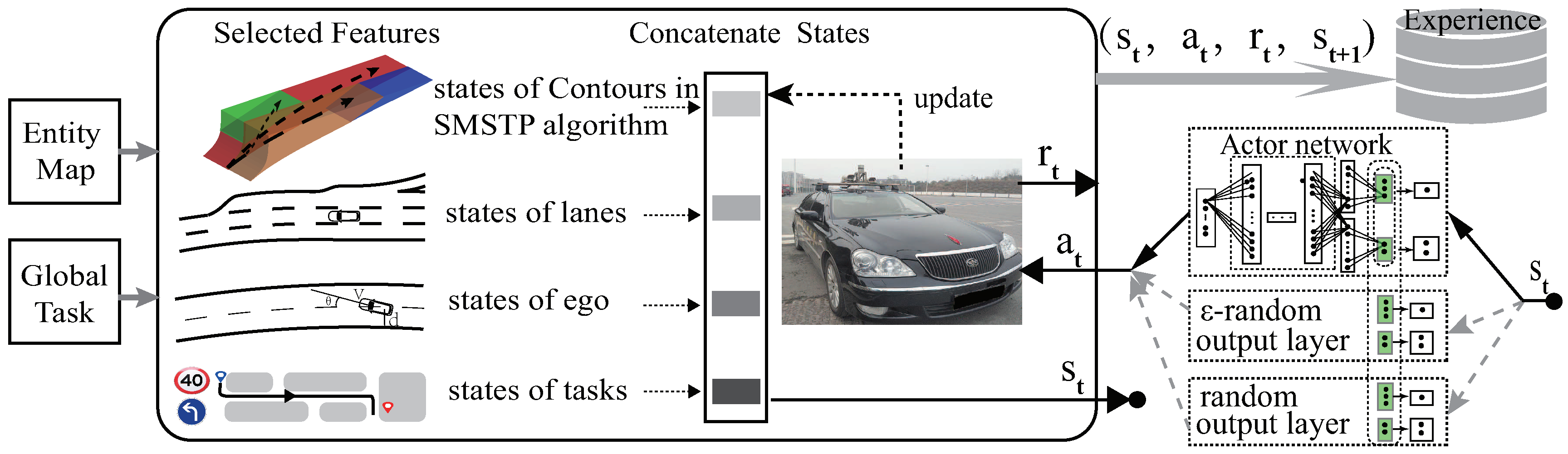
A policy with safety ensured can be implemented in autonomous vehicles. Generating a policy by combining path planning features can be one feasible choice. If given the traffic participants and environments, a system can provide all possible maneuvers with corresponding reasonable paths; then, the decision policy can be reinforced with learning methods by selecting the best maneuver. Proceeding with previous work, the synchronous maneuver searching and trajectory planning algorithm (SMSTP) [23], we propose a new planning-features-based behavior decision method whose architecture is shown in Figure 2. SMSTP outputs no-collision trajectories which represent the safe policy in yellow of Figure 1, while the target of our proposed PFBD approach was to learn the optimal policy in green.

In the SMSTP algorithm, three key parameters, the contour to drive, the expected pose and velocity at predicting horizon in the contour, are selected empirically. To learn an optimal policy, we creatively propose to use the DRL algorithm to learn the aforementioned three key parameters instead. The SMSTP algorithm provides a basic policy with a safety guarantee, while PFBD aims at optimizing the behavioral decision towards the optimum. Once the three key parameters are decided, a no-collision trajectory can be optimized numerically.

To the authors’ knowledge, the deep combination of trajectory planning and behavioral decisions for autonomous vehicles is proposed for the first time here. In brief, we summarize the contributions of the proposed approach in this paper as follows:

• We came up with a compact semantic framework of the feature representation which includes planning space’s states, lanes’ states, ego vehicle’s states and task’s states. The states selected from planning space are necessary and representative for making behavioral decisions in various traffic scenarios.
• The proposed PFBD method selects a route generated from the planning space with a safety guarantee. Besides, it learns better policy through exploring the environment instead of struggling with the rules.
• The proposed method learns a policy through deep reinforcement learning. The semantic training data can be sampled from both simulations and real traffic. The simulated samples help the policy generalize the unknown scenarios.
• We applied the method to autonomous driving in situations, such as lane changing, zebra passing and ramp-merging. Both simulation and real-time tests were performed. The PFBD method achieved competitive performance compared to rule-based methods.

1.1. Reinforcement Learning Basics

RL originates from the trial-and-error search with delayed rewards, and it is dedicated to learning the optimal policy, which maximizes a long-term reward in the subsequent decisions. The agent learns a control policy by continuously interacting with its environment, and the policy maps states to actions from interactions.

The agent is in a state $s_t\in S$ of itself and its environment at the time $t\in [0,1,2,\cdots ]$, and it has a possible action $a_t\in A_{s_t}\subseteq A$ on state $s_t$, where S and A are the sets of all the environment states and available actions, respectively. An agent in a new state $s_{t+1}$ observes an immediate reward $r_t=r(s_t,a_t)\in R$ after executing the action $a_t$. A new state transition tuple $(s_t,a_t,r_t,s_{t+1})$ is then sampled to train for a control strategy, which is defined by a policy $\pi$ mapping the states to the actions $\pi :S$→$P\left(A\right)$. The agent aims at maximizing the long-term discounted return defined as:$R_t={\sum }_{t=1}^{inf}{\gamma }^{t-1}{r}_t$, where $\gamma \in [0,1]$ is the discount. On the policy $\pi$, the state-action value function:

$$Q^{\pi }(s_t,a_t)=E_{\pi }\left[r_t\right|s_t,a_t],$$

(1)

describes how good the policy is after taking an action $a_t$ in state $s_t$.

The policy $\pi$ is often acquired by recursively solving the Bellman equations:

$$Q^{\pi }(s_t,a_t)=E_{s_{t+1}\sim S,a_t\sim \pi }[r(s_t,a_t)+\gamma E_{\pi }\left[Q^{\pi }(s_{t+1},a_{t+1})\right]].$$

(2)

The driving policy in a realistic traffic situation can be viewed as a deterministic one. The policy then can be described using a function $\mu :S\leftarrow A$, and the expectation of action can be avoided:

$$Q^{\mu }(s_t,a_t)=E_{s_{t+1}\sim S}[r(s_t,a_t)+\gamma E_{\mu }\left[Q^{\pi }(s_{t+1},a_{t+1})\right]].$$

(3)

Deep Reinforcement Learning

For a value-only based RL algorithm, such as deep Q-learning, it adopts a deep neural network (DQN) instead of a table to estimate the value to each state-action pair. DQN uses a greedy $\mu \left(s\right)=arg{max}_{a}Q(s,a)$ in discrete action spaces. Approximated by parameter ${\theta }^Q$, one agent optimizes the function by minimizing the loss:

$$Loss\left({\theta }^Q\right)=E_{\mu }\left[{(Q(s_t,a_t)-y_t)}^2\right],$$

(4)

where the term $y_t=r(s_t,a_t)+\gamma Q(s_{t+1},\mu \left(s_{t+1}\right)|{\theta }^Q)$ is called the target, as the loss tries to make the value function be more like this target. The long-term accumulation of reward leads to high variance. Besides, DQN only works well with few actions; thus, failing in continuous action spaces.

DDPG [19], a model-free off-policy algorithm, can be used for environments with continuous action spaces. DDPG has two pairs of actor-critic networks with the same structure. The critic network approximates the state-action value function $Q(s,a|\theta )$ by parameter $\theta$, which updates by minimizing (4). The actor network approximates the agent’s policy $\mu \left(s\right|\omega )$ by parameter $\omega$, which deterministically maps the observed state s to an certain action a. The actor network is updated by the derivative of (3) respectively to the actor parameters:

$${\nabla }_{\omega }\mu \approx \frac{1}{N}\sum _i{\nabla }_{a}Q(s,a|\theta ){{|}_{s=s_i,a=\mu \left(s_i\right)}{\nabla }_{\omega }\mu \left(s\right|\omega )|}_{s=s_i},$$

(5)

where N is the number of state transitions.

Two main technologies are employed by DDPG to enable a stable learning process. The first one is the replay buffer, which is the set E of previous experiences in the form of state transitions $(s_t,a_t,r_t$ and $s_{t+1})$. The learning policy may shift towards and even over-fit to training samples. Therefore, old experiences are indispensable for robustness. To balance the learning process, new experiences are given a higher probability than older ones of being sampled in a minibatch. The other technology is the target network originally used in DQN. The target term in (4) depends on the same parameters to be learned while the network is being trained. This problem makes loss optimization unstable. The solution is to use another pair of networks $Q^{{}^{\prime }}(s,a|{\theta }^{{}^{\prime }})$ and ${\mu }^{{}^{\prime }}\left(s\right|{\omega }^{{}^{\prime }})$ with a time delay. A second network, called the target network, lags behind the first one, which is called the evaluation network. The target network updates by a smooth average:

$$\begin{array}{cc}\hfill {\theta }^{{}^{\prime }}& =\tau \theta +(1-\tau ){\theta }^{{}^{\prime }}\hfill \\ \hfill {\omega }^{{}^{\prime }}& =\tau \omega +(1-\tau ){\omega }^{{}^{\prime }}\hfill \end{array}$$

(6)

where $\tau \ll 1$.

To address the over-approximation of actor-critic networks, the twin-delayed deep deterministic policy gradient algorithm (TD3) [24] based on DDPG employs three technologies. The delayed policy update changes the target networks slowly every d steps, and this makes networks steadier by avoiding over accumulating the rewards. The policy smoothing supposes similar states should have similar actions by adding noise to the target actions in target Q networks:

$$\begin{array}{cc}\hfill y_t& =r(s_t,a_t)+\gamma Q(s_{t+1},\tilde{a}|{\theta }^{{}^{\prime }})\hfill \end{array}$$

(7)

$$\begin{array}{cc}\hfill \tilde{a}& =\left(\mu \left(s_{t+1}\right)\right|{\omega }^{{}^{\prime }})+ϵ\hfill \\ \hfill ϵ& \sim \mathrm{clip}\left(\mathcal{N}\right(0,\sigma ),-c,c),\hfill \end{array}$$

(8)

where $\sigma$ is a parameter for noise, c is the boundary for clipping. Clipped double Q-Learning uses two randomly initialized critic networks as estimates and always takes the minimum one to update the target:

$$y_t=r(s_t,a_t)+\gamma \underset{i=1,2}{min}Q(s_{t+1},\tilde{a}|{\theta }_i^{{}^{\prime }}).$$

(9)

2. Problem Formulation

2.1. Vehicle Models

The vehicle uses a kinematic bicycle model for forward motion and lateral movement:

$$x_{t+1}=x_t+v_{t}cos\left({\theta }_t\right)\nabla T$$

(10)

$$y_{t+1}=y_t+v_{t}sin\left({\theta }_t\right)\nabla T$$

$$v_{t+1}=v_t+a_t\nabla T$$

$${\theta }_{t+1}={\theta }_t+\frac{tan\left({\delta }_t\right)}{L}{v}_t\nabla T,$$

where x and y are the vehicle’s lateral and longitudinal positions; v and a are the velocity and acceleration; and $\theta$ and $\delta$ are the vehicle’s heading and steering angles, respectively. L is the wheelbase and $\nabla T$ is the time step size. Since this paper focuses on the decision level, the dynamic of other traffic vehicles is assumed to be controlled by fixed acceleration speed. To simulate generally, different behavior modes of traffic vehicles are used; namely: aggressive mode, regular mode and modest mode. The behavior modes are characterized by different acceleration speeds, safe distances to follow a front vehicle, safe distances to overtake a front vehicle and safe distances to avoid near back vehicles. Each participant vehicle emerges randomly around the ego agent with random target speed. These simulated vehicles are also enabled to change lanes within a random time interval following general traffic rules in their own behavior modes. These settings enable the vehicle to explore more potential types of traffic scenarios, which are prerequisites to learn the optimum policy.

2.2. Planning Space

In real traffic flows, an experienced driver not only observes the nearest vehicle in each lane but also looks far ahead in a defensive manner. Looking far ahead helps drivers notice potential hazards and drive smoothly. Therefore, the traffic vehicles in front of the ego agent’s planning scope should be considered.

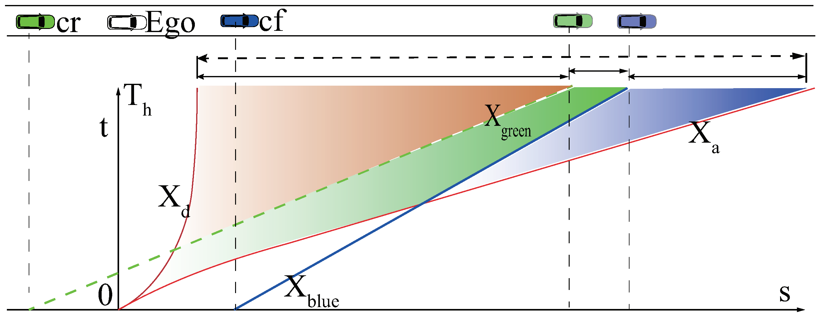
In previous work [23], the horizon for decision and planning was fixed as $T_h$. The planning scope in Figure 3 shows the range between the end pose ($X_d$) of agent decreasing to zero velocity, and the end pose ($X_a$) of an agent accelerating to the maximum velocity allowed within $T_h$. Vehicles inside such a scope influence the agent’s behavior and the states for decision.

3. Methodology

3.1. States

The agent’s behavioral decision depends on all relevant traffic entities. An entity can be a traffic participant, a pedestrian, a car or a bicycle with pose and velocity information. The lanes and signs, such as stop signs and speed limit signs with particular instructive information, are also entities. However, to generate a safe decision based on the topological routes, entities’ information must be translated into planning features with specific meanings, as summarized in

Table 1. The feature states for behavioral decision. Five contours exist in each lane. At most three lanes are considered. The ‘∘’ represents that a feature is scaled to $[-1,1]$ before it is concatenated into states.

States (of)	Features	Meaning
Contour(${\mathbf{s}}_{\mathbf{c}}$)	$c_{rd}$ (∘)	the planning scope’s rear-end distance
	$c_{fd}$ (∘)	the planning scope’s front-end distance
	$c_{fv}$ (∘)	the planning scope’s front-end velocity
Lane(${\mathbf{s}}_{\mathbf{l}}$)	$l_l$ (∘)	lane’s effective length
	$l_a$	lane’s attribute(accelerating, decelerating,..)
	$l_c$ (∘)	lane’s curvature
	$l_v$ (∘)	lane’s speed limitation
Ego agent(${\mathbf{s}}_{\mathbf{e}}$)	$e_v$ (∘)	agent’s absolute velocity
	$e_a$	agent’s acceleration speed
	$e_h$ (∘)	agent’s heading relative to lane’s direction
Task (discrete,(${\mathbf{s}}_{\mathbf{c}}$))	$t{k}_d$	the degree of task (mandatory, discretionary)
	$t{k}_l$	the lane-error to target lane of task
	$t{k}_p$	the right of way in task
Task (continuous,(${\mathbf{s}}_{\mathbf{c}}$))	$t_p$	the position of special task
	$t_v$	the target velocity to follow at $t_p$
	−	the preserved states for future use

.

Features representing these entities are crucial for the agent’s decision, which are pre-processed as following.

3.1.1. States of Contours in Planning Space

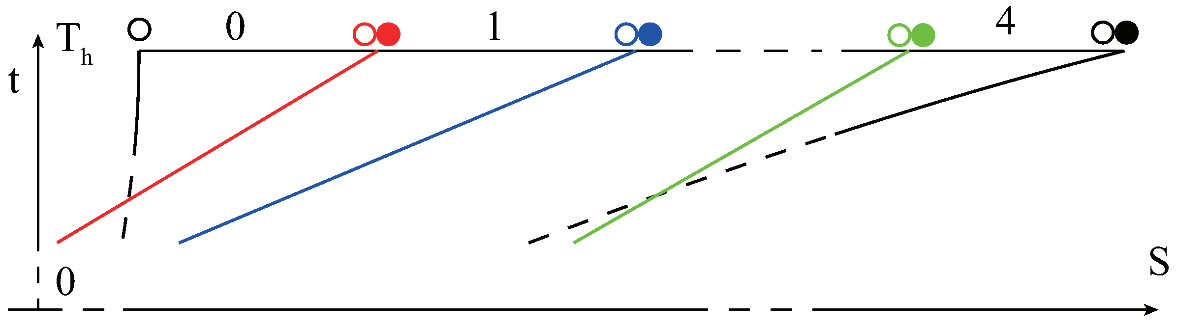
To make a safe decision, the features for available planning space are extracted from results of SMSTP algorithm, which guarantee safe topological routes in Figure 3. Each contour corresponding one route has three features, as shown in Figure 4. Two of them are the rear-end and front-end poses of a contour, $c_{rd}$ and $c_{fd}$, respectively. One feature is the recommended velocity $c_{fv}$ at the front end. If the contour is split by a vehicle at the front end, then this feature is related to the velocity of that vehicle; otherwise, it depends on the maximum velocity that ego agent can reach at time $T_h$.

As the input sizes of networks are fixed, the upper number of contours in each lane is limited to five according to a safe following distance, empirically. Besides, two adjacent contours have one shared feature: that the front-end distance $c_{fd}^i$ of i’th contour equals the rear-end distance $c_{rf}^{i+1}$ of $i+1$’th contour (Figure 4). The state for contours in each lane has total 11 features. Therefore, 33 features consist of the state of contours ${\mathbf{s}}_{\mathbf{c}}$ when three lanes (left lane, current lane and right lane) are considered. The features of distance can be quite enormous compared to some states, such as lane ID $[-1,0,1]$. Hence, the distance $d\in [0,334]$ and velocity $v\in [0,33.4]$ are mapped to $[-1,1]$:

$$out=2\frac{in-i{n}_{min}}{i{n}_{max}-i{n}_{min}}-1,in\in (d,v).$$

(11)

3.1.2. States of Lanes

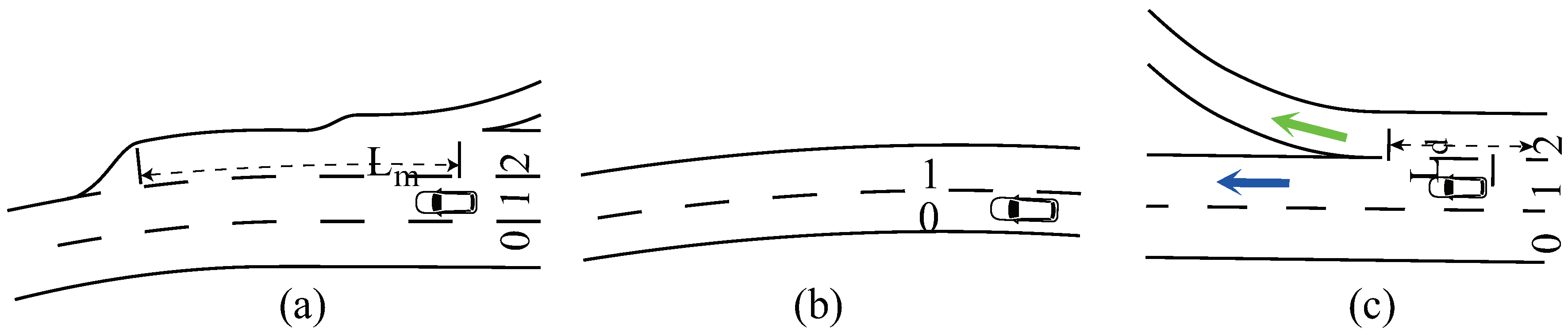
The state of lanes ${\mathbf{s}}_{\mathbf{l}}$ contains all structural constrains that decide where a vehicle can go. One key feature is the length of a lane $l_l$. Taking scenario (a) in Figure 5 for example, when the agent goes in lane $\mathbf{1}$, the merging lane’s (lane $\mathbf{2}$) length is, $L_m$, from the agent’s position to the right lane’s end. The left lane does not exist in scenario (b), hence the length is zero. In scenario (c), when the task is going straight along the arterial road, the rightest detached lane’s length is, $L_d$, from the agent’s position to the separation point. However, when the task is leaving the arterial road, the lengths of lane $\mathbf{0}$ and lane $\mathbf{1}$ are both $L_d$. So that feature $l_l$ depends on the global task and lane’s structure simultaneously.

One inherent feature of lanes is the curvature $l_c$ which limits the maximum speed. The other two features are the lane’s attribute $l_a$ and the speed limit $l_v$ of a lane. The rightmost lanes in scenario (a) and scenario (c) are the accelerating lane and decelerating lane in the on-off ramp area, respectively, which means vehicles in these lanes should adjust their speeds to the suggested ones as quickly as possible.

3.1.3. States of the Ego Agent

The state of ego agent ${\mathbf{s}}_{\mathbf{e}}$ includes absolute velocity $e_v$, acceleration speed $e_a$ and the angle between vehicle’s heading lane’s direction $e_h$. Here, acceleration and velocity are both scaled to $[-1,1]$. $e_h$ is restricted between −0.26 rad and 0.26 rad first, which is then scaled to $[-1,1]$.

3.1.4. States of Tasks

Driving along a road without following traffic rules is relatively simple. However, autonomous vehicles of this kind are not acceptable in realistic situations. An agent’s capability includes both going into a target lane and reaching the given position at a specific speed. The former is guided by task features in a discrete form, while the latter is instructed by target features in a continuous form.

Three separate task-level features are employed here. The task-level $t{k}_d$ means to which degree the agent should follow a given task. When the agent’s task is to leave the arterial road in scenario (c) of Figure 5, the mandatory task-level requires the agent to arrive at the rightmost lane before coming to the separation point. The discretionary task-level means that the agent can select any available lane to maintain a high cruise speed in scenario (c). The other one, lane-error $t{k}_l$, is the relative distance to the target lane. Lane-error represents how many lanes there are between the current lane and the target lane, which is the main punishment for task requirements. Another key feature is the prioritization $t{k}_p$. When two vehicles’ distances to intersections have no significant difference, a vehicle with the right of way is encouraged to go in priority. Otherwise, it should go after vehicles in other roads.

Two continuous target features, the target pose $t_p$ to reach and the target velocity $t_v$ to follow, guide the agent to arrive at the position with given speed. Taking intersection cross, for example, a recommended speed can be 25 km/h for the sake of safety and traffic rules, if the agent traverses at higher speeds, some punishment will be given. These two features also represent speed limits from traffic signs. Including four preserved ones, the state of task ${\mathbf{s}}_{\mathbf{tk}}$ has nine features.

The final state for MDP is ${\mathbf{s}}_{\mathbf{t}}=<{\mathbf{s}}_{\mathbf{c}}^{\mathbf{t}},{\mathbf{s}}_{\mathbf{l}}^{\mathbf{t}},{\mathbf{s}}_{\mathbf{e}}^{\mathbf{t}},{\mathbf{s}}_{\mathbf{tk}}^{\mathbf{t}}>$ with a total of 57 features.

3.2. Actions

The action $a_t=<a_l^t,a_d^t,a_v^t>$ uses three sub-actions jointly to decide an agent’s behavior and optimizing parameters in a select contour. The first discrete action $a_l^t\in [-1,0,1]$ selects a lane to go among the left lane, the current lane and the right lane if they exist. The second continuous action $a_d^t\in [-1,1]$ represents the target position to reach $T_h$ between $X_d$ and $X_a$. The third continuous action $a_v^t\in [-1,1]$ stands for the target velocity to follow at time $T_h$. The inverse transformation of (11) is used to get either the predicted distance ${\overline{a}}_d^t\in [0,334]$ or the velocity ${\overline{a}}_v^t\in [0,33.4]$ by

$$out=\frac{in+1}{2}(o_{max}-o_{min})+o_{mim},in\in (a_d,a_v),$$

(12)

where $o_{max}$ and $o_{min}$ are the maximal and minimal expected values of inputs. In fact, due to the values of action $a_d^t$ and action, $a_v^t$ can hardly be 1 or $-1$ through hyperbolic sine function. We enlarge both $o_{max}$ and $o_{min}$ a bit and truncate the outputs to expected ranges.

Action $a_l^t$ selects the target lane, and it has several contours in the corresponding planning scope. The undetermined contour for the trajectory optimizer depends on ${\overline{a}}_d^t$. If ${\overline{a}}_d^t$ locates inside one contour of the planning scope in Figure 4, then this contour is selected. Otherwise, either the nearest or the furthest contour is selected and ${\overline{a}}_d^t$ is adjusted to either $c_{rd}^0$ or $c_{fd}^i$ (i depends on the number of contours in the lane). In the trajectory optimizer layer of the SMSTP, the chosen contour, adjusted ${\overline{a}}_d^t$ and ${\overline{a}}_v^t$, determine the final trajectory in predicted horizon $T_h$.

3.3. Rewards Design

The ego agent employs an action and gets a reward $r_t$ at time t, which evaluates the current state and action. $r_t$ guides the policy to learn proper actions for higher rewards and reflects to what degree the agent drives as we expect.

A well-designed reward represents the desired policy for complex driving tasks. Therefore, $r_t$ is a compromise among agent’s safety, traveling efficiency, and task achievement in linear combination form:

$$\begin{array}{cc}\hfill r_t& =r_s^t+r_e^t+r_t^t\hfill \end{array}$$

(13)

$$\begin{array}{cc}\hfill r_s^t& =\left\{\begin{array}{cc}-10,\hfill & \mathrm{a}\mathrm{collision}\hfill \\ -2,\hfill & \mathrm{a}\mathrm{lane}\mathrm{change}\hfill \\ 0,\hfill & \mathrm{else}\hfill \end{array}\right.\hfill \end{array}$$

(14)

$$\begin{array}{cc}\hfill r_e^t& =min(e_v-\frac{{\sum }_{i=1}^n\left(v_i\right)+l_v}{n+1},0)\hfill \end{array}$$

(15)

$$\begin{array}{cc}\hfill r_t^t& +=\left\{\begin{array}{cc}max(-5,-2\ast t{k}_l),\hfill & \mathrm{lane}-\mathrm{error}\hfill \\ max(-5,-|e_v-t_v),\hfill & \mathrm{target}\mathrm{speed}\mathrm{error}\hfill \\ \cdots ,\hfill & \mathrm{else},\hfill \end{array}\right.k\hfill \end{array}$$

(16)

where $r_s^t$ is the safety penalty, $r_e^t$ is the reward for agent’s driving efficiency, $r_t^t$ is the penalty for deviation from task’s target and $v_i$ is the velocity of the i’s traffic participant. As frequent lane changes can cause danger in traffic flow, a small penalty is set in $r_s^t$ of (14) to discourage unnecessary lane changes. A reasonable agent drives as fast as possible within the speed limit of a lane. However, being a cooperative member of the traffic flow is much safer. Hence, $r_e^t$ in (15) leads the agent to drive at the average speed of traffic, and to pursue the maximal speed of the lane, whether there are traffic participants or not. $r_t^t$ provides an agent the ability to perform different tasks, which depends on the requirements. For example, $-5t{k}_l$ in (16) punishes the agent for deviating from the target lane when the agent should be in the target lane. $-|e_v-t_v|$ punishes the agent for being unable to follow given speed limitations. To achieve other tasks, $r_t^t$ should adjust the penalty term accordingly. Each term in $r_t^t$ is not less than $-5$.

3.4. Neural Networks

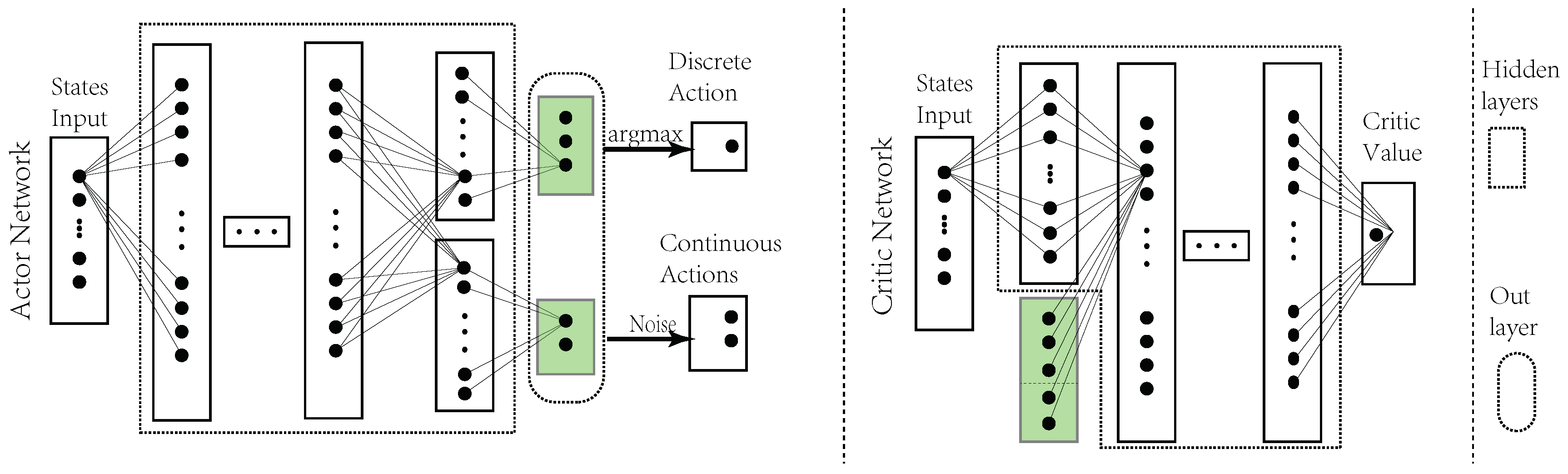
The actor and critic networks are presented in Figure 6. A state ${\mathbf{s}}_{\mathbf{t}}$ enters the actor network, which has five neurons as the output layer in green. A softmax function takes the first three neurons as input and outputs the discrete action $a_l^t$. Two continuous actions $a_d^t$ and $a_v^t$ are the last two neurons adding some noises. The critic network takes a state ${\mathbf{s}}_{\mathbf{t}}$ as input, and concatenates the first hidden layer with the output layer of actor network as the input of second hidden layer. A scalar value is output as the action-value (Q-value).

The actor network has three mutual hidden layers, and each layer has 256, 512 and 128 neurons, respectively. The private layers connecting discrete and continuous actions both have 64 neurons. The critic network has three hidden layers, and each has 256, 128 and 64 neurons, individually. Rectified linear unit (ReLu) activation functions are used in the hidden layers. Meanwhile the output layer of actor network uses tanh functions to constrain the value of actions.

3.5. Algorithm Procedure

The procedure of PFBD method for autonomous vehicle safe decision is Algorithm 1. The algorithm includes two main parts. The first part is for sampling and evaluation. Experiences of state transitions are sampled before the policy is trained. Algorithm 1, firstly, initializes the actor-critic networks and sets a task for agent along with the penalty function for different tasks. After initializing the state $s_0$ in each episode, action $a_t$ is generated according to sampling mode among random sampling and $ϵ$-random sampling. $a_t$ shifts agent to next state $s_{t+1}$, and a reward $r_t$ follows. When the number of state transitions $({\mathbf{s}}_{\mathbf{t}},{\mathbf{a}}_{\mathbf{t}},{\mathbf{r}}_{\mathbf{t}},{\mathbf{s}}_{\mathbf{t}+\mathbf{1}})$ reaches $N_{max}$, the transitions are stored as a group into “Experience” on the local disk. If a policy has been trained, we set sampling mode to “Evaluation” to evaluate its performance.

For the training part, $N_{env}$ groups of samples in Experience are loaded from disk. The newer stored samples are given a higher priority to balance the shifting of policy. Then, the parameters of evaluation and target networks are updated in sequence.

Algorithm 1 Planning features based behavior decision algorithm (PFBD)

Initialization:  Initialize evaluation actor-critic networks’ parameters ${\theta }_1$, ${\theta }_2$, $\omega$ randomly   Initialize target actor-critic networks’ parameters ${\theta }_1^{{}^{\prime }}\leftarrow {\theta }_1$, ${\theta }_2^{{}^{\prime }}\leftarrow {\theta }_2$, ${\omega }^{{}^{\prime }}\leftarrow \omega$ 1: for task $k=1$ to $N_k$ do 2:  Set a Task and sampling mode, load the traffic map, reset traffic participants 3:  Initialize the agent’s state $s_0$ 4:  for step $t=0$ to T do 5:   generate action $a_0$ according to sampling mode 6:   switch (sampling mode) 7:   case Random sampling: randomize the output layer of the actor network 8:   case $ϵ$-random sampling: randomize the output layer of actor network with probability $ϵ$ 9:   case Evaluation: use the trained policy (forward through actor network) 10:   end switch 11:   Employ action $a_t$ to next state $s_{t+1}$ based on SMSTP algorithm, calculate the reward $r_t$ 12:   Save transition $({\mathbf{s}}_{\mathbf{t}},{\mathbf{a}}_{\mathbf{t}},{\mathbf{r}}_{\mathbf{t}},{\mathbf{s}}_{\mathbf{t}+\mathbf{1}})$, $++n_s$ 13:   if $n_s==N_{max}$ then 14:    Store $N_{max}$ transitions as a group into Experience, $n_s=0$ 15:   end if 16:  end for 17:  for epoch $ep=1$ to $N_{epoch}$ do 18:   Load $N_{env}$ groups of Experience from disk with priority, randomly sample a minibatch of $N_{minibatch}$ transitions 19:   Update critic in evaluation network by minimizing (4), target is updated by (9) 20:   Update actor in evaluation network following (5) 21:   Update the target networks following (6) 22:  end for 23: end for

4. Simulation and Experiment

Since the proposed approach focuses on behavioral decision and planning with only abstract entities for autonomous driving, we tested the method with our vehicle simulation platform instead of real traffic. A schematic view of sampling and evaluation architecture is depicted in Figure 2.

4.1. Simulation Setting

4.1.1. Environment

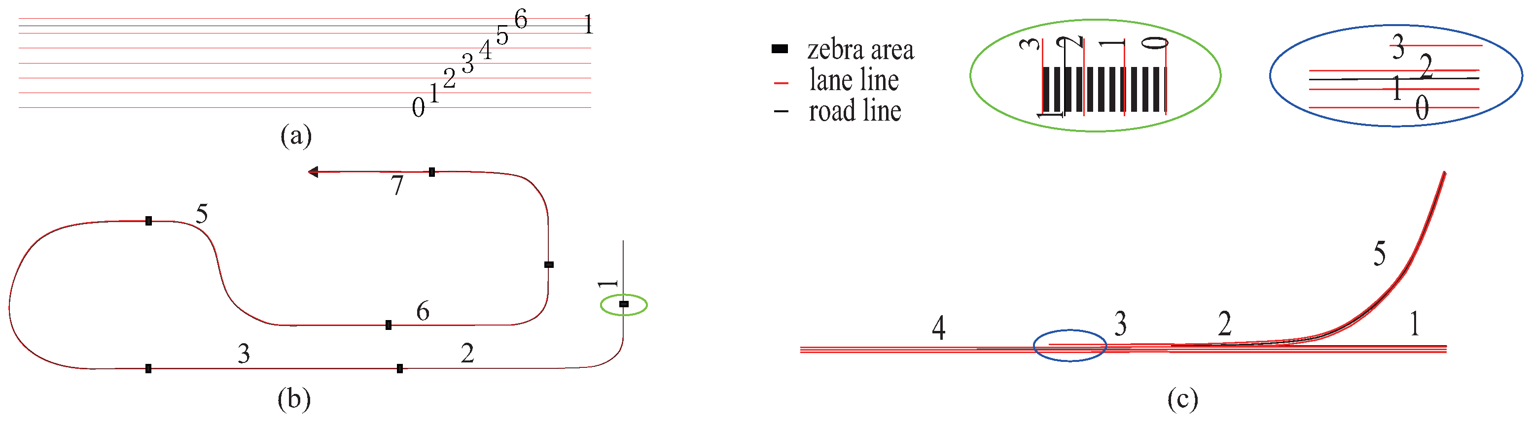
Experiments included three typical scenarios of different traffics, as shown in Figure 7. The first one was a straight six-lane road scenario (Scenario A). The second one was a curve road scenario (Scenario B). Scenario B had seven zebras in the straight part of the road. The last one was a merging road (Scenario C). The lane’s width was set to four meters. The maximum sensible ranges of the front and back were set to 200 m and 100 m, respectively.

4.1.2. Traffic Participants

The other traffic participants and their behaviors were set as anticipated in Section 2.1. The participants changed their behavior modes at a probability $p=0.005$. (If five traffic participants exist, the probability of at least one changing its behavior in one second is 0.2217.) The changing of behavior mode ensures abundant experiences of different scenes. A vehicle was reset when it got out of the agent’s range.

The participants employ an expert system to make behavioral decisions and to execute longitudinal control. The expert system considers the distances and velocities of the nearest vehicles in the surrounding lane. The decision system has been well tested in real traffic experiments [25].

4.1.3. Hyper-Parameters for TD3

A minibatch of 64 state transitions was randomly selected from 32 groups of experiences to train the policy every two steps. The optimization method for TD3 is the Adam algorithm [26], and the learning rates for actor and critic networks are ${10}^{-2}$ and ${10}^{-4}$, respectively. The discount for future reward was set to 0.99. We used deep learning framework, libtorch (Pytorch for C++) [27], to train the agents.

4.2. Performance Index

To evaluate the capabilities of PFBD method, the following metrics are introduced.

• Collision Rate [%]: the collision rate is defined as

  $$R_c=\frac{CR}{V\ast T\ast L},$$

  (17)

  where $CR$ is the number of crashes that happened, V is the traffic volume in the agent’s sensible range, $T\ge 1$ is the time in hours the agent drives and L is the total distance traveled. This is the most critical metric for evaluating the agent’s performance.
• Average velocity (m/s): the average velocity represents how fast the agent drives and to what degree the expected velocity is matched.
• Average distance between collisions (km): the distance between two collisions is to avoid the influence of agent’s velocity and duration time.
• Rule-violation rate (%): the violation rate indicates the agent’s capability of achieving given tasks, such as decreasing when a zebra is coming, keeping in specific lanes and leaving the ramp’s accelerating lane before coming to its end.

4.3. Simulation and Evaluation

In the simulation, we trained four different agents with four corresponding polices. Three agents’ policies, $P_A$, $P_B$ and $P_C$ were trained individually on three typical scenarios (see Section 4.1), respectively. To validate the versatility of PFBD, one more agent’s policy $P_T$ was trained on all three scenarios. Besides, we compared the performance of PFBD method with the rule-based expert system and an untrained random policy.

An episode is reached in the following three cases:

• Case 1: the agent is made to unavoidably collide with a vehicle in 1.5 s.
• Case 2: the agent has successfully made more than 20 decisions.
• Case 1: the agent updates for 600 steps without collisions.

The last two rules prevent an episode with too many running steps.

To generate the desired behavior, the reward function for scenarios B and C was modified accordingly. For scenario B with zebras on the road, $r_t^t$ in (16) is added with a new term:

$$\begin{array}{cc}\hfill r_{t\left(zebra\right)}^t& =max(-5.,-0.5\ast \frac{v_{error}}{1+sqrt(min(d_{zebra},100))})\hfill \\ \hfill v_{error}& =\sqrt{max({10}^{-4},v-v_{zebra})},\hfill \end{array}$$

(18)

where $v_{zebra}$ is the recommended velocity to pass a zebra area and $d_{zebra}$ is the distance to a zebra. For task entering the main road in scenario C, $r_t^t$ in (16) is added with:

$$r_{t\left(ramp\right)}^t=-0.5\ast \sqrt{-min(100,d_{ramp})+100},$$

(19)

where $d_{ramp}$ is the distance to ramp’s end.

At the first stage, we sampled more than one million state transitions in each scenario randomly. Then, the agents, $P_A$, $P_B$ and $P_C$ were trained from samples in each scenario according to Algorithm 1, respectively. $P_T$ was trained on samples from all three scenarios. Then, we used the trained agents to sample with a probability $ϵ$ randomly selecting the actions. The agents did not stop being trained until the loss stopped decreasing for 10 epochs.

4.3.1. Performance of PFBD on Different Scenarios

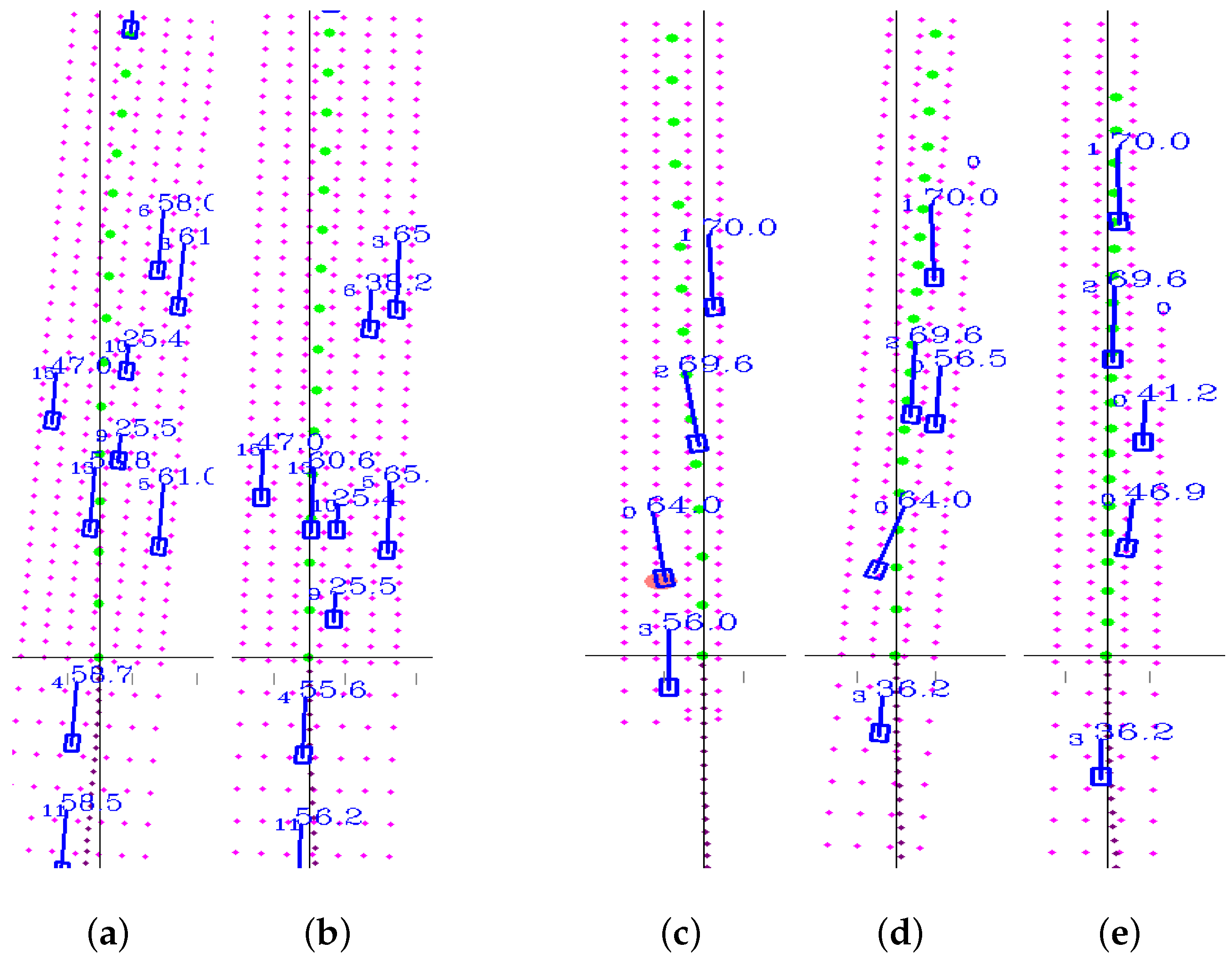
Figure 8 shows the decision and planning result of trained agents in the simulation environment. Figure 8a,b illustrates that the agent takes over the front vehicle (ID = 9) and follows a relatively quicker vehicle (ID = 13). Figure 8c–e shows that the agent merges into the middle lane timely before the ramp(right lane) ends.

The statistical results for four agents are listed in

Table 2. The evaluation results of training-acquired policy in different scenarios. - represents no consideration.

	${\mathbf{P}}_{\mathbf{A}}$	${\mathbf{P}}_{\mathbf{B}}$	${\mathbf{P}}_{\mathbf{C}}$	${\mathbf{P}}_{\mathbf{T}}$ (Scenario A)	${\mathbf{P}}_{\mathbf{T}}$ (Scenario B)	${\mathbf{P}}_{\mathbf{T}}$ (Scenario C)
Collision Rate	$0.23\%$	$0.39\%$	$1.17\%$	1.3%	$1.6\%$	$1.68\%$
Average Velocity (m/s)	18.1	15.1	14.5	14.9	12.0	11.8
Av. Dist No Col (ks)	18.2	13.6	14.9	11.5	10.8	9.1
Rule Violation	-	3.15%	2.4%	-	5.33%	3.68%

. Generally, the trained agents achieved the designed maneuvers. The collision rate and average distance without collision show that the agent can learn proper policy to avoid collisions. Scenario A is easier for the agent to drive in since the agent achieves the highest average velocity and lowest collision rate. For scenarios B and C, the agent has to slow down for the zebra or limit its speed in the ramp. ${\mathbf{P}}_{\mathbf{T}}$ can also learn proper behaviors on all three scenarios without an evident decrease in performance.

Note that the average distance without collision is relatively short in the simulation. The main cause is that a traffic participant sometimes emerges too close to the agent since it is randomly reset. For the abundance of sample distribution, the nearest distance to the agent is 20 m. When the agent is much quicker than the simulated vehicle in the front, a collision can be hard to avoid. The rule violation is also difficult to define clearly. In our simulation, for a successful result in the zebra scenario, the duration of the agent’s velocity being smaller than the recommended velocity has to be kept up for at least two seconds.

4.3.2. Comparison with the Expert’s Policy

DRL-based PFBD method can explore optimal policy via interacting with environments. Nevertheless, the rule-based expert’ policy often struggles in dynamic situations with heavy traffic. Therefore, the performance of the trained policy was compared to the expert’s policy. The agents $P_A$, $P_B$ and $P_C$ ran for at least ${10}^5$ iterations and at least 2500 maneuvers executed. The expert’s policy described in Section 4.1.2 and a random policy (untrained) were both evaluated.

One critical concern is that the reward of lane-keeping must be recorded in a balanced manner. We did not record a reward in every iteration. On the contrary, either the agent kept in a lane for every 40 steps or a non-lane-keeping maneuver was selected; the reward of lane-keeping was recorded at one time.

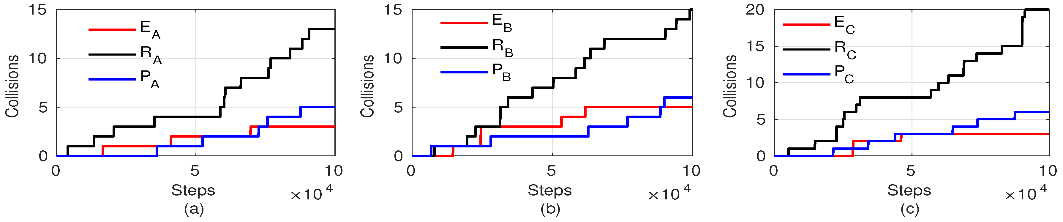
Figure 9 depicts the collision times after the agents ran for ${10}^5$ iterations in three testing scenarios. It shows that the learned agents for all three scenarios significantly decreased the collision times after training. Besides, the learned agents achieved competitive performance, as did the conservative traditional expert. In fact, a large number of the collisions derived from a too-close-in-front vehicle after resetting. Although the low-level SMSTP algorithm can plan all non-collision topological paths, whether the trajectory can be well executed is undetermined (the agent cannot decelerate quickly enough). Therefore, collision times depend on the performance of a policy. The simulation results verify that the agents can learn proper policy after training.

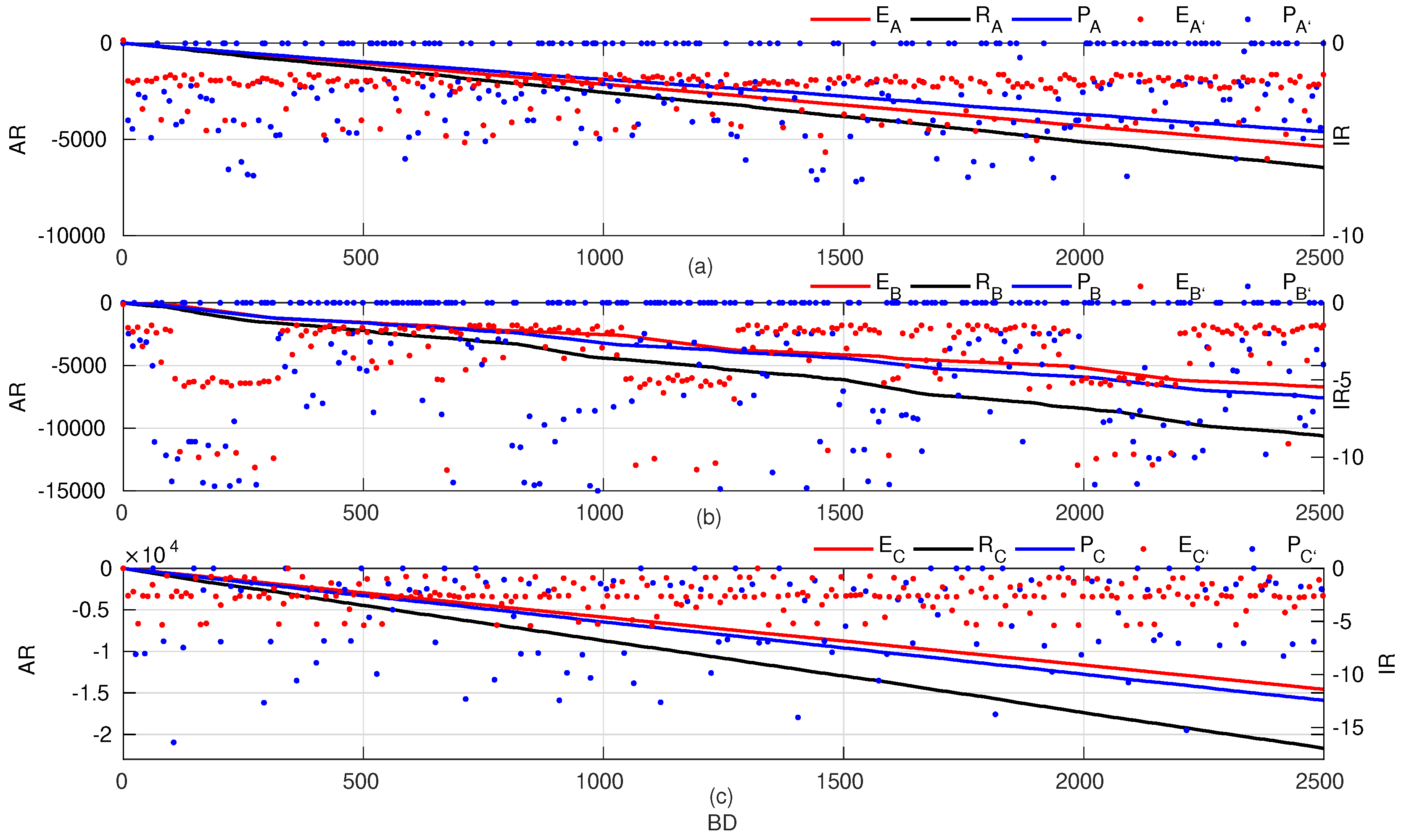
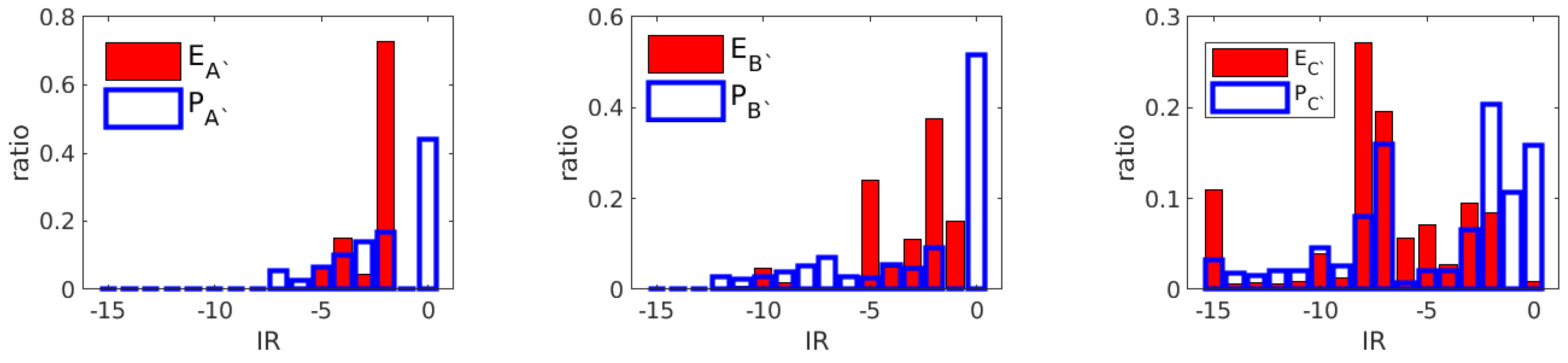
For the rewards of the learned agents, as shown in Figure 10, most immediate rewards (in blue points) achieved zero punishments in scenario A and B, while the expert’s immediate rewards (in red points) seldom got no punishment. A statistical distribution of immediate rewards is listed in Figure 11. Both agent $P_A$ and agent $P_B$, more than 40% of the time, received zero punishments. This implies that the agents successfully found an optimal policy in the corresponding states. In contrast, the expert’s policy mostly had a small immediate reward, as the expert behaved conservatively and got trapped in dynamic traffic at a relatively low speed most of the time. In the ramp merging scenario, the agent and expert both had a scattered distribution of immediate rewards, which reflected the difficulty in the ramp-merging task. Both policies had to compromise for a successful merging maneuver.

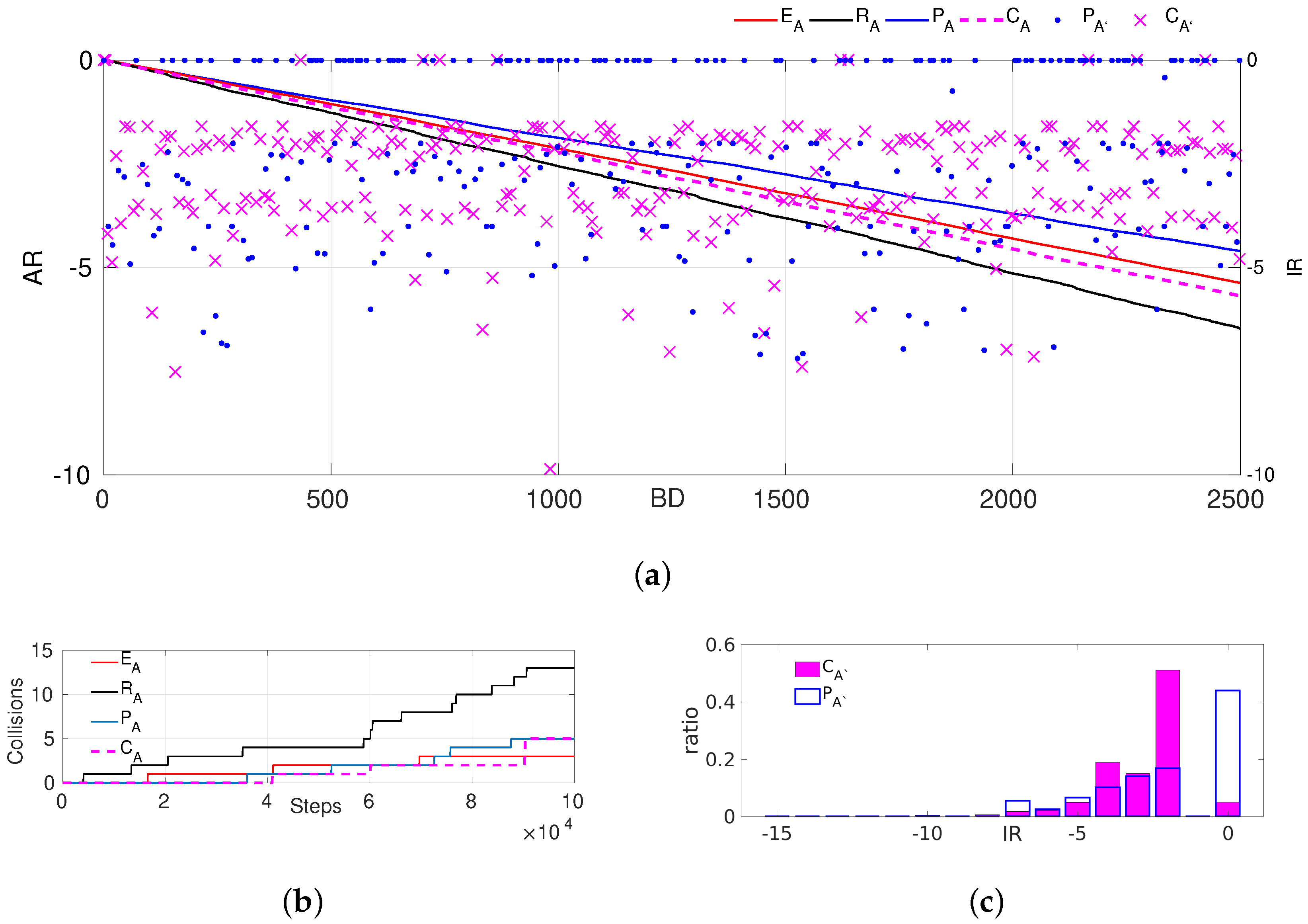
4.3.3. Comparison with standard DRL

To validate whether the states of contours help to make a better decision, we compared the proposed PBFD with a standard DRL where all the parameters were selected as the same as those in the PBFD except for the dynamic features from the planning layer being not concerned in the standard DRL. To achieve this, we specifically set, in the DRL, the planning scope’s front-end distance $c_{fd}$ to zero with small noise. With the above design, we trained a new agent $C_A$ in scenario A, whose behaviors are displayed together with those of the PBFD and the expert in Figure 12.

The results show that agent $C_A$ had almost the same collision times as $P_A$ in ${10}^5$ running steps. It can also be seen in Figure 12a,c that agent $C_A$ had about a $6\%$ chance of achieving zero punishment, which is better than expert’s policy (in Figure 11), which could hardly get any zero punishment outcomes. However, agent $C_A$ behaved worse than agent $P_A$, as $40\%$ of immediate rewards of agent $P_A$ were zero. This means that agent $P_A$ with full knowledge of contour states has larger probabilities of making optimal behavioral decisions. Thus, the creative design of contour is vital to learn better behavior decisions.

4.4. Real-time Experiment On HQ3 Autonomous Vehicle

To validate the capacity of the proposed PFBD algorithm for autonomous vehicle decision making, the real-time experiment on HQ3 autonomous vehicle was conducted in the suburbs with regular traffic. HQ3 [25] was equipped with necessary sensors, including cameras, LIDAR, radars, inertial measurement unit (IMU), etc.

To use the learned agents in real-time test, we kept the same states in both simulation and the real test, and we ignored those states that did not exist in simulations, such as an intersection with turn commands. The two main tests in the suburbs were keeping in the target lane near a zebra (corresponding to Scenario A and B) and merging onto the main road from a side road (corresponding to Scenario C). The agent’s maximum speed was limited to 60 km/h. The road network avoided untrained tasks, such left turning or right turning that did not exist in simulation.

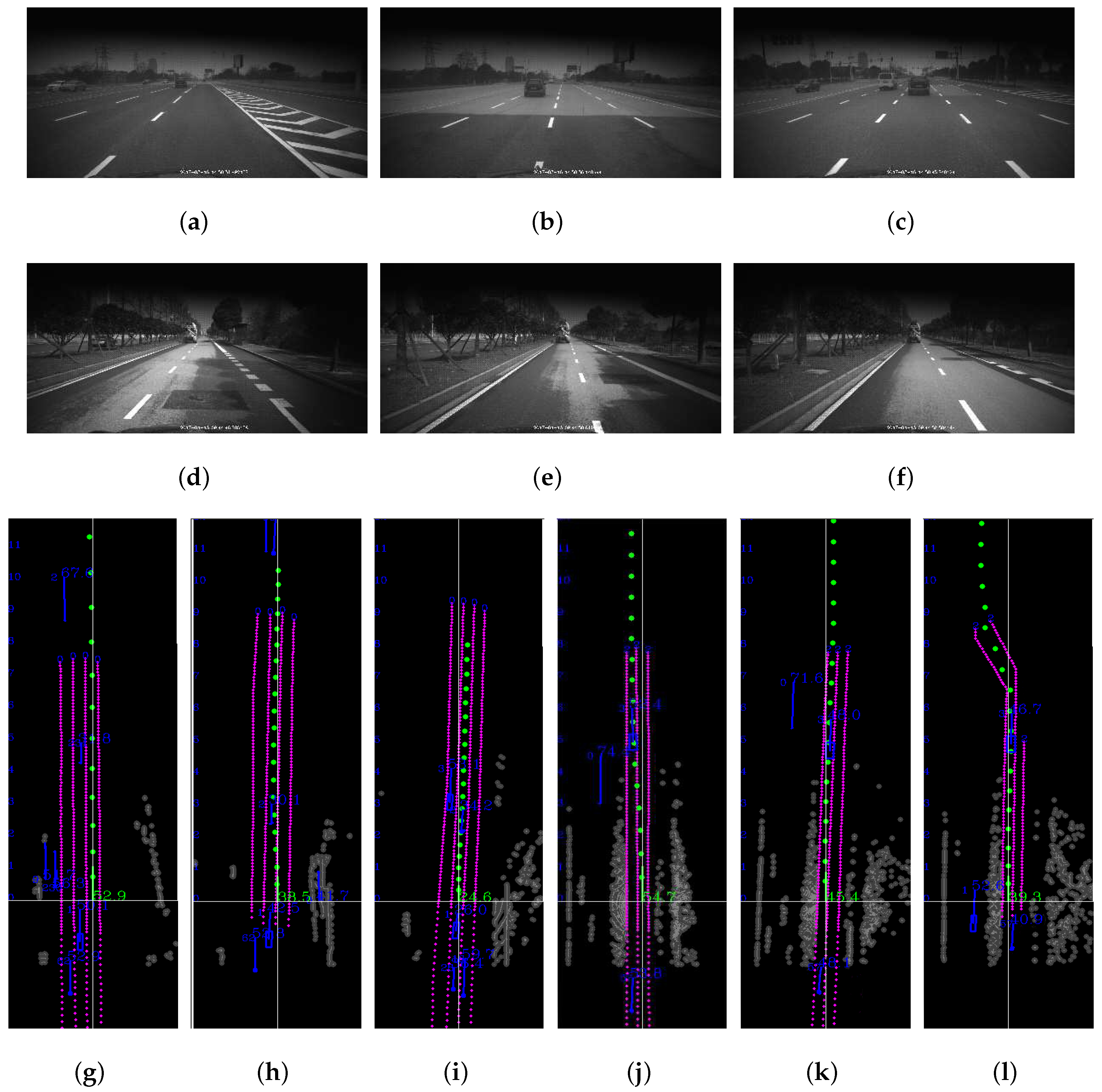
Figure 13 shows the agent’s behavioral decision and trajectory planning results for the two separate maneuvers. The blue short lines indicate the speeds and directions of the detected surrounding vehicles on the road. In the first test, HQ3 successfully merged to the middle lane. Besides, as the zebra area was coming (see Figure 13c, the planned trajectory led HQ3 to slow down (see green trajectory of Figure 13i). In the second test, our agent tried to merge into the left main road (see Figure 13d–f). HQ3 changed to the left curve lane before the road network of the side road coming to end. As in the real-time test shown, the trajectory planner based on the learned agent can successfully generate a smooth and safe trajectory for HQ3.

5. Conclusions

In this paper, a novel planning features-based, deep behavior decision method trained with TD3 was proposed to select an optimal maneuver for autonomous vehicles in dynamic traffic. The PFBD uses rule-based topological trajectories as basic guarantees and learns optimal policy with DRL, which helps to bring learning methods to the autonomous vehicle’s core module, behavioral decisions and trajectory planning. The behavioral decision problem was modeled as an MDP process, and the training algorithm was proposed. Due to the creative design of input states and actions, the behavior decision is inherently associated with drivable routes in the topological planning space. Thus, the policy’s decision is consistent with trajectory planning, and the path is a safer one. The evaluation results have demonstrated that the proposed method can learn proper behaviors. Besides, comparisons to the expert’s policy and the standard DRL validate the effectiveness of PFBD and show its capability to find optimal strategies with larger possibilities. The real-time test also validated the effectiveness of the proposed PFBD.

Since the agent’s performance is competitive compared to the rule-based expert’s policy, the future work will extend the current discrete behavioral decisions to consecutive ones, which shall evaluate the present behaviors and potential behaviors in every time step. Therefore, some emergent situations could be tackled immediately rather than executing the ongoing behavior to the end. In the meanwhile, more traffic scenarios can be used to test the generalization performance of the proposed method.

References

- Montemerlo, M.; Becker, J.; Bhat, S.; Dahlkamp, H.; Dolgov, D.; Ettinger, S.; Haehnel, D.; Hilden, T.; Hoffmann, G.; Huhnke, B.; et al. Junior: The Stanford entry in the Urban Challenge. J. Field Robot. 2008, 25, 569–597. [Google Scholar] [CrossRef] [Green Version]
- Kurt, A.; Özgüner, Ü. Hierarchical finite state machines for autonomous mobile systems. Control Eng. Pract. 2013, 21, 184–194. [Google Scholar] [CrossRef]
- Pomerleau, D.A. ALVINN: An Autonomous Land Vehicle in a Neural Network. In Advances in Neural Information Processing System 1; Morgan Kaufmann Publishers Inc.: San Francisco, CA, USA, 1989; pp. 305–313. [Google Scholar]
- Bojarski, M.; Testa, D.D.; Dworakowski, D.; Firner, B.; Flepp, B.; Goyal, P.; Jackel, L.D.; Monfort, M.; Muller, U.; Zhang, J.; et al. End to End Learning for Self-Driving Cars. arXiv 2016, arXiv:1604.07316. [Google Scholar]
- Caltagirone, L.; Bellone, M.; Svensson, L.; Wahde, M. LIDAR-based driving path generation using fully convolutional neural networks. In Proceedings of the 2017 IEEE 20th International Conference on Intelligent Transportation Systems (ITSC), Yokohama, Japan, 16–19 October 2017; pp. 1–6. [Google Scholar]
- Silver, D.; Huang, A.; Maddison, C.J.; Guez, A.; Sifre, L.; Van Den Driessche, G.; Schrittwieser, J.; Antonoglou, I.; Panneershelvam, V.; Lanctot, M.; et al. Mastering the game of Go with deep neural networks and tree search. Nature 2016, 529, 484. [Google Scholar] [CrossRef] [PubMed]
- Qi, X.; Luo, Y.; Wu, G.; Boriboonsomsin, K.; Barth, M. Deep reinforcement learning enabled self-learning control for energy efficient driving. Transp. Res. Part C Emerg. Technol. 2019, 99, 67–81. [Google Scholar] [CrossRef]
- Nazari, M.; Oroojlooy, A.; Snyder, L.; Takac, M. Reinforcement Learning for Solving the Vehicle Routing Problem. In Proceedings of the 32nd Conference on Neural Information Processing Systems (NeurIPS 2018), Montréal, QC, Canada, 3–8 December 2018; pp. 9839–9849. [Google Scholar]
- Aradi, S.; Becsi, T.; Gaspar, P. Policy Gradient Based Reinforcement Learning Approach for Autonomous Highway Driving. In Proceedings of the 2018 IEEE Conference on Control Technology and Applications (CCTA), Copenhagen, Denmark, 21–24 August 2018; pp. 670–675. [Google Scholar]
- Wolf, P.; Kurzer, K.; Wingert, T.; Kuhnt, F.; Zollner, J.M. Adaptive Behavior Generation for Autonomous Driving using Deep Reinforcement Learning with Compact Semantic States. In Proceedings of the 2018 IEEE Intelligent Vehicles Symposium (IV), Changshu, China, 26–30 June 2018; pp. 993–1000. [Google Scholar]
- Wang, P.; Chan, C.-Y.; Fortelle, A.D. A Reinforcement Learning Based Approach for Automated Lane Change Maneuvers. In Proceedings of the 2018 IEEE Intelligent Vehicles Symposium (IV), Changshu, China, 26–30 June 2018; pp. 1379–1384. [Google Scholar]
- Shalev-Shwartz, S.; Shammah, S.; Shashua, A. Safe, multi-agent, reinforcement learning for autonomous driving. arXiv 2016, arXiv:1610.03295. [Google Scholar]
- Li, N.; Oyler, D.W.; Zhang, M.; Yildiz, Y.; Kolmanovsky, I.; Girard, A.R. Game Theoretic Modeling of Driver and Vehicle Interactions for Verification and Validation of Autonomous Vehicle Control Systems. IEEE Trans. Contr. Syst. Technol. 2018, 26, 1782–1797. [Google Scholar] [CrossRef] [Green Version]
- You, C.; Lu, J.; Filev, D.; Tsiotras, P. Advanced planning for autonomous vehicles using reinforcement learning and deep inverse reinforcement learning. Robot. Auton. Syst. 2019, 114, 1–18. [Google Scholar] [CrossRef]
- Zhu, M.; Wang, X.; Wang, Y. Human-like autonomous car-following model with deep reinforcement learning. Transp. Res. Part C: Emerg. Technol. 2018, 97, 348–368. [Google Scholar] [CrossRef] [Green Version]
- Huang, Z.; Xu, X.; He, H.; Tan, J.; Sun, Z. Parameterized Batch Reinforcement Learning for Longitudinal Control of Autonomous Land Vehicles. IEEE Trans. Syst. Man, Cybern. Syst. 2019, 49, 730–741. [Google Scholar] [CrossRef]
- Xu, C.L.Z.H.X.; Wang, J. Lateral control for Autonomous Land Vehicles via Dual Heuristic Programming. Int. J. Robot. Autom. 2016, 36. [Google Scholar] [CrossRef] [Green Version]
- Lian, C.; Xu, X.; Chen, H.; He, H. Near-Optimal Tracking Control of Mobile Robots Via Receding-Horizon Dual Heuristic Programming. IEEE Trans. Cybern. 2016, 46, 2484–2496. [Google Scholar] [CrossRef] [PubMed]
- Lillicrap, T.P.; Hunt, J.J.; Pritzel, A.; Heess, N.; Erez, T.; Tassa, Y.; Silver, D.; Wierstra, D. Continuous control with deep reinforcement learning. Comput. Sci. 2016, 8, A187. [Google Scholar]
- Sallab, A.; Abdou, M.; Perot, E.; Yogamani, S. Deep Reinforcement Learning framework for Autonomous Driving. Electron. Imaging 2017, 2017, 70–76. [Google Scholar] [CrossRef] [Green Version]
- Bai, Z.; Cai, B.; Wei, S.G.; Chai, L. Deep Learning Based Motion Planning For Autonomous Vehicle Using Spatiotemporal LSTM Network. In Proceedings of the 2018 Chinese Automation Congress (CAC), Xi’an, China, 30 November–2 December 2018; pp. 1610–1614. [Google Scholar]
- Chen, L.; Hu, X.; Tian, W.; Wang, H.; Cao, D.; Wang, F. Parallel planning: A new motion planning framework for autonomous driving. IEEE/CAA J. Autom. Sin. 2019, 6, 236–246. [Google Scholar] [CrossRef]
- Qian, L.; Xu, X.; Zeng, Y.; Li, X.; Sun, Z.; Song, H. Synchronous Maneuver Searching and Trajectory Planning for Autonomous Vehicles in Dynamic Traffic Environments. IEEE Intell. Transp. Syst. Mag. in press.
- Fujimoto, S.; van Hoof, H.; Meger, D. Addressing Function Approximation Error in Actor-Critic Methods. In Proceedings of the Thirty-Fifth International Conference on Machine Learning, Stockholm, Sweden, 10–15 July 2018. [Google Scholar]
- Qian, L.; Fu, H.; Li, X.; Cheng, B.; Hu, T.; Sun, Z.; Wu, T.; Dai, B.; Xu, X.; Tang, J. Toward Autonomous Driving in Highway and Urban Environment: HQ3 and IVFC 2017. In Proceedings of the 2018 IEEE Intelligent Vehicles Symposium (IV), Changshu, China, 26–30 June 2018; pp. 1854–1859. [Google Scholar]
- Kingma, D.P.; Ba, J. Adam: A Method for Stochastic Optimization. In Proceedings of the 3rd International Conference for Learning Representations, San Diego, CA, USA, 7–9 May 2015. [Google Scholar]
- Paszke, A.; Gross, S.; Chintala, S.; Chanan, G.; Yang, E.; DeVito, Z.; Lin, Z.; Desmaison, A.; Antiga, L.; Lerer, A. Automatic differentiation in PyTorch. In Proceedings of the NIPS-W 2017, Long Beach, CA, USA, 4–9 December 2017; p. 4. [Google Scholar]
Figure 1.
Explanation of polices in decision space. The yellow area represents safe policy. The green area represents the optimal policy. The dotted ellipse is the rule-based or experience-based policy. The solid ellipse is the learned policy.
Figure 2.
The sample and evaluation architecture of decision and planning for autonomous vehicles. A contour [23] is one transitable spatio-temporal area for autonomous vehicles in the synchronous maneuver searching and trajectory planning algorithm (SMSTP) algorithm.
Figure 3.
The planning scope (the dotted line with a double arrow) of the ego agent (in white). Two surrounding vehicles are in dim green and in dim blue at time 0. At time , these two vehicles are in light colors. For the one-lane situation, the only available route is in the green contour. The rear-end distance and the front-end distance are the green vehicle’s and blue vehicle’s distances at time in the future, respectively. The solid lines with double arrows are the planning scopes for three contours.
Figure 4.
Five contour states in a lane’s planning scope. The hollow circles and solid circles represent distance and velocity states of a contour in corresponding colors, respectively. The colored lines stand for trajectories of other traffic participants.
Figure 5.
Lane states in different lane structures. (a) An in-ramp road. (b) A two-lane roa. (c) An off-ramp road.
Figure 6.
The structure of actor–critic networks. The actions are sampled from the output layer (in green color) of the actor network. The output layer is concatenated with the second layer of critic network. The discrete action is calculated from output layer through a softmax function. The continuous actions are sampled from the other two unions with small noises
Figure 7.
Different traffic scenarios used to train and evaluate the performance agent’s policy. (a) A straight road with six lanes. (b) A curved road with zebras in the straight parts. (c) A merging road. The red lines represent lane lines. The black lines are roads.
Figure 8.
Two typical maneuvers. (a,b) An overtaking maneuver in a six-lane road with heavy traffic. (c–e) show a lane merging maneuver at ramp. Each simulated vehicle is labeled with ID and speed (km/h) information. The red points are the lane lines. The big green points and small purple ones represent the planned trajectory and the historical trajectory, respectively.
Figure 9.
The collision times after iterations for three different traffic scenarios. , and represent the policies for expert, random and learned agents, respectively. (a) The collision times in scenario . (b) The collision times in scenario . (c) The collision times in scenario
Figure 10.
The rewards of reinforcement learning (RL) policy compared to expert’s policy and a random policy for 2500 maneuvers. (a) Rewards in Scenario . (b) Rewards in Scenario . (c) Rewards in Scenario . The blue and red points represent the immediate rewards of the trained agent and the expert, respectively. Only one eighth of the points for IR are illustrated for clarity. AR: accumulated rewards, BD: behavioral decisions, IR: immediate rewards.
Figure 11.
The distribution of immediate rewards for both learned agents and the expert in three testing scenarios.
Figure 12.
The comparison results of states with or without the profile’s information. (a) Rewards in Scenario A. The • and magenta × are the immediate rewards of agent and agent , respectively. (b) The collision times in Scenario A. (c) The distribution of immediate rewards of agent and agent .
Figure 13.
Snaps of two real-time maneuvers in the suburbs. (a–c and d–f) are the front views of (g–i and j–l), respectively. The red dotted lines are the lane lines. The green points are the planned trajectory. The gray areas are obstacles.