An Image Compression Method for Video Surveillance System in Underground Mines Based on Residual Networks and Discrete Wavelet Transform

 , ,
, ,
Abstract
:1. Introduction
1.1. The Image Compression Demand from Underground Mines
1.2. From Conventional Image Compressing to Compressed Sensing
1.3. Data-Driven Approaches
1.3.1. Convolution Neural Network based Image Compression
1.3.2. Recurrent Neural Network Based Image Compression
1.3.3. Generative Adversarial Network Based Image Compression
1.4. The Objectives and the Organization of the Paper
2. The Proposed Image Compression Method
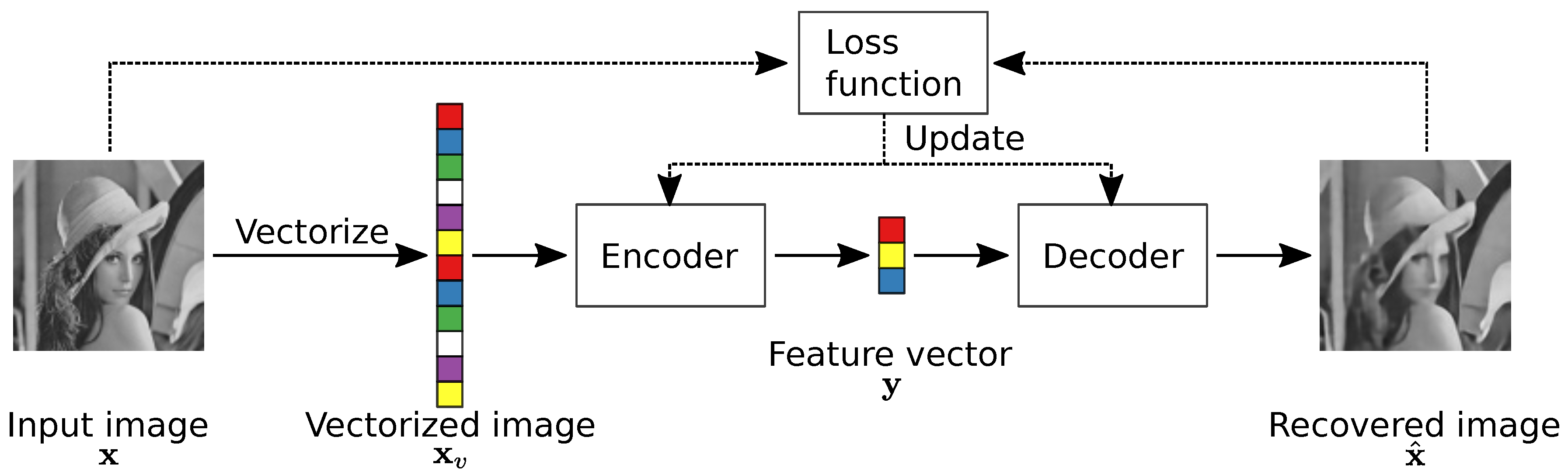
2.1. Overview
2.2. The Network Architecture
2.2.1. The Encoder Module
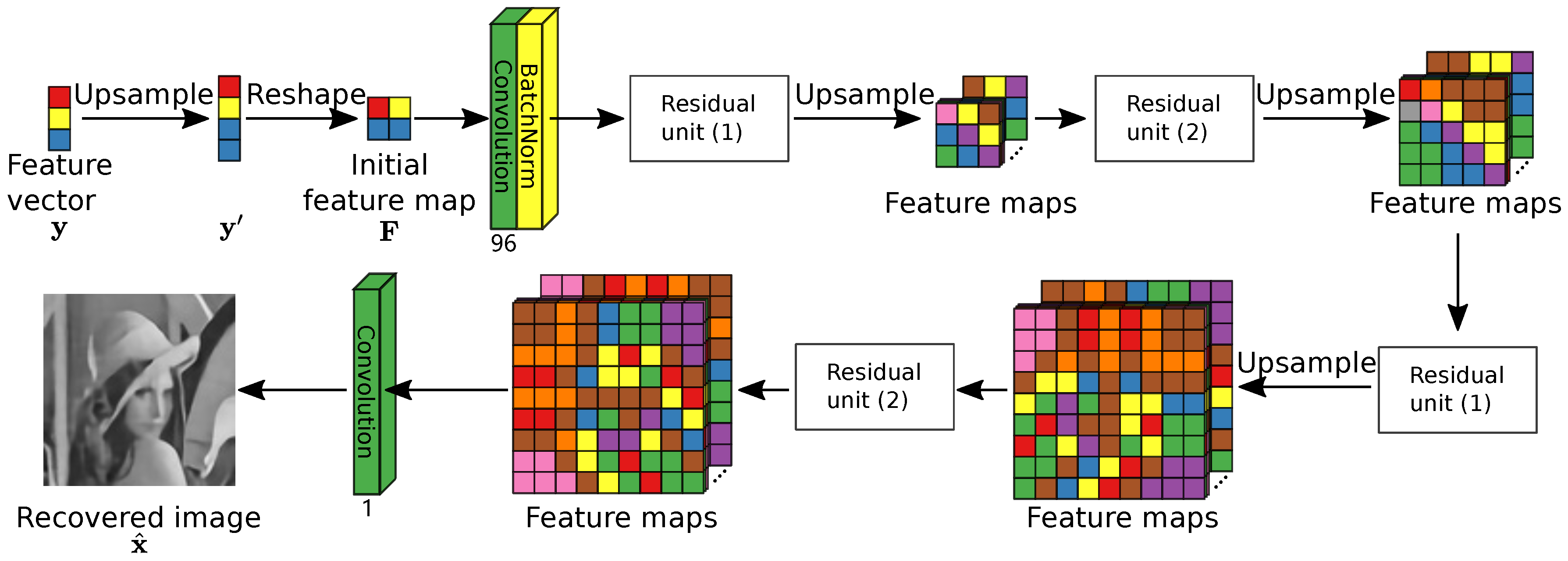
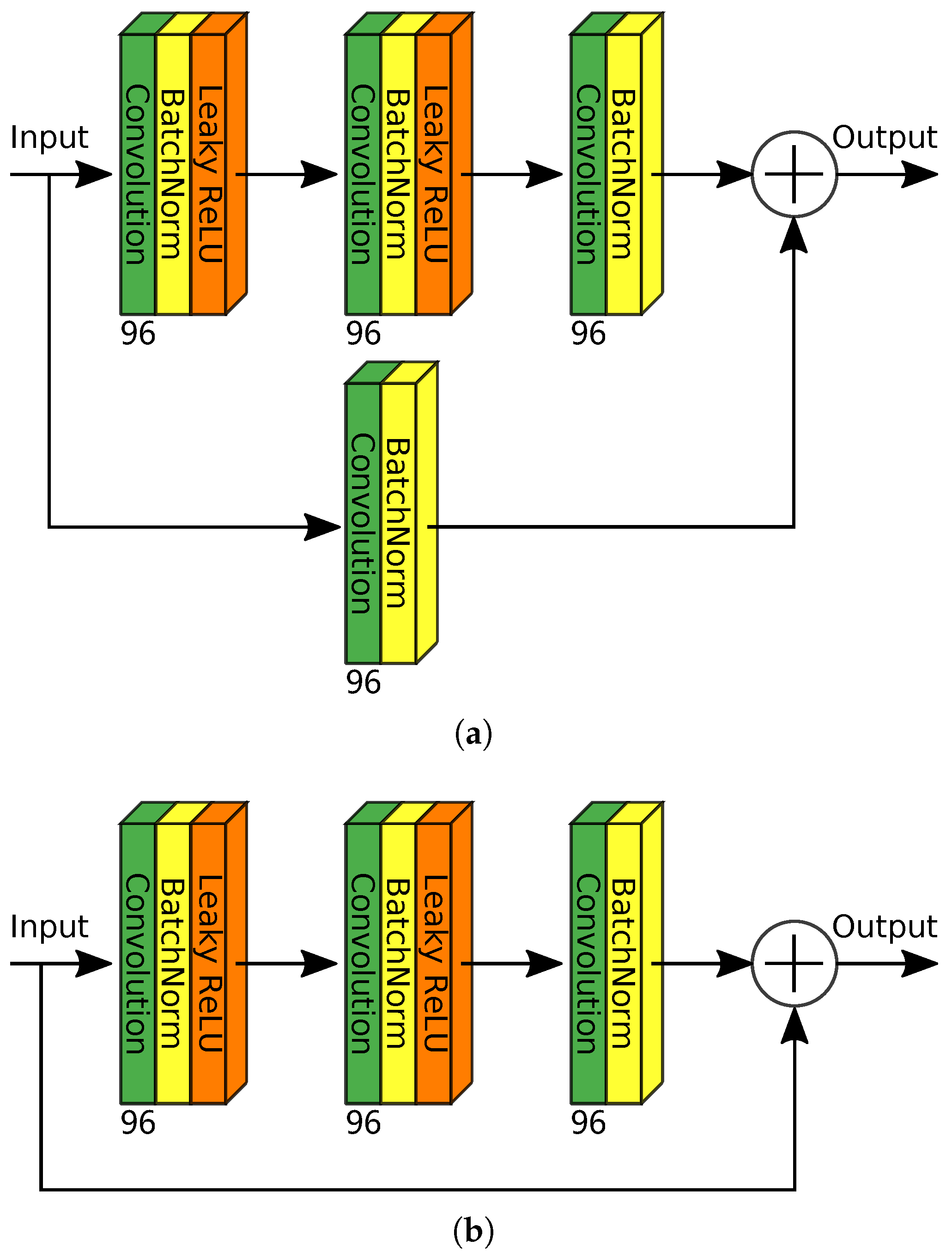
2.2.2. The Decoder Module
2.3. The Proposed Loss Function
2.3.1. Combination of Two Types of Loss Functions
2.3.2. Loss
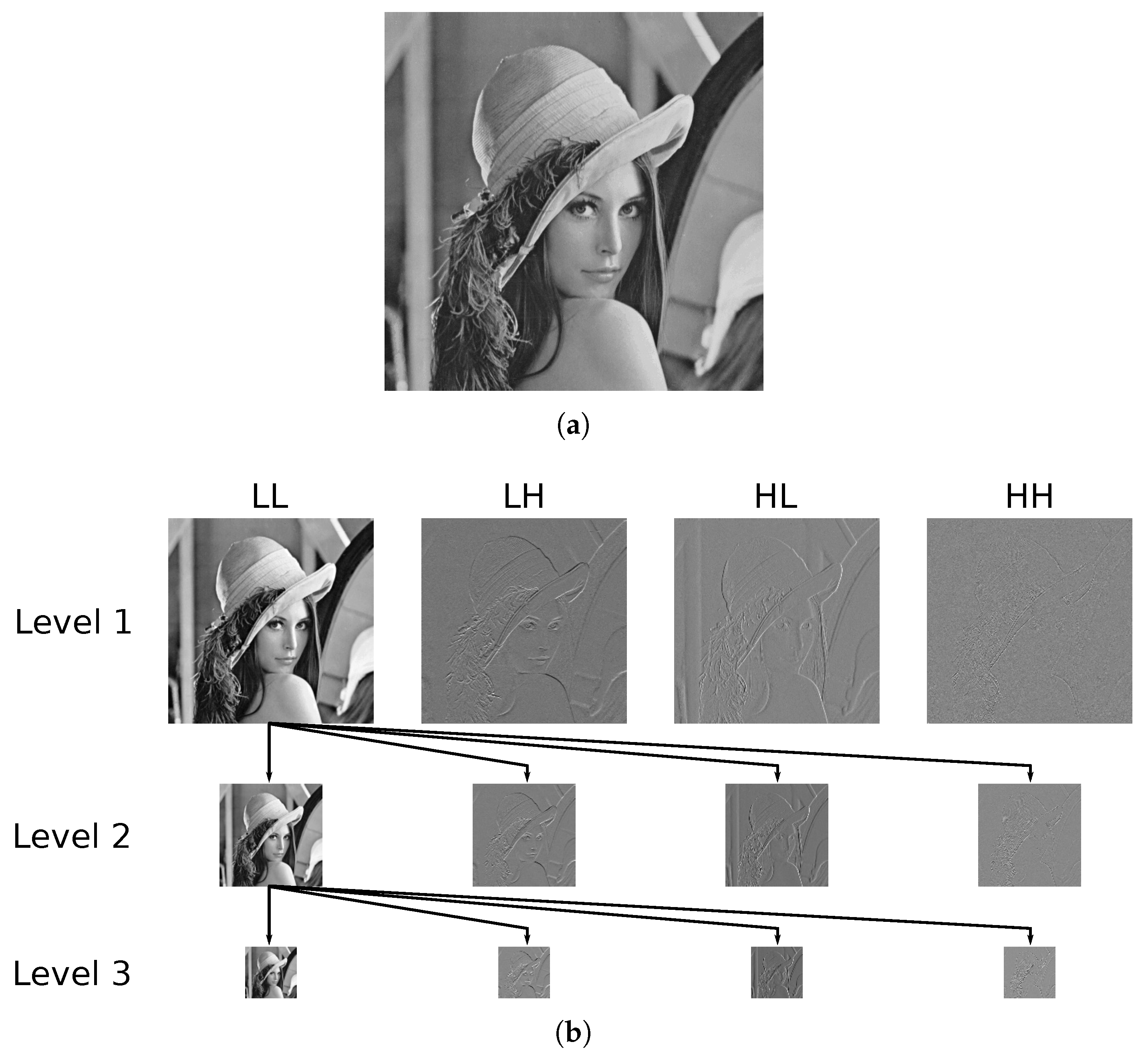
2.3.3. Discrete Wavelet Similarity (DW-SSIM) and DW-SSIM Loss
| Algorithm 1: The procedure to compute discrete wavelet similarity (DW-SSIM). |
| Input: The original image img-ori and the recovered image img-rec of the same height H and width W (); the decomposition level J; the stride s that the window will move in each iteration; the window length l; the weights and in Equation (10) Output: The DW-SSIM similarity S between img-ori and img-rec |
 |
2.4. Learning the Parameters
3. Results
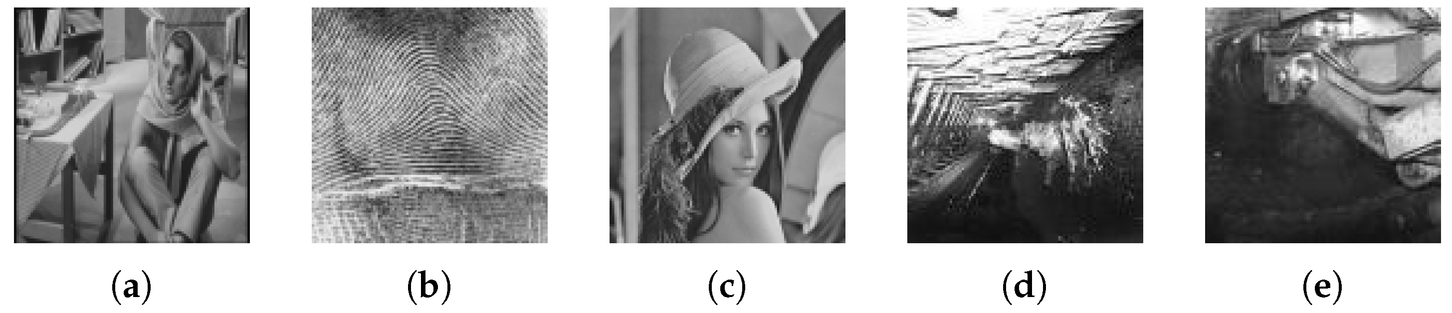
3.1. Overview
3.2. Quantitative Evaluation
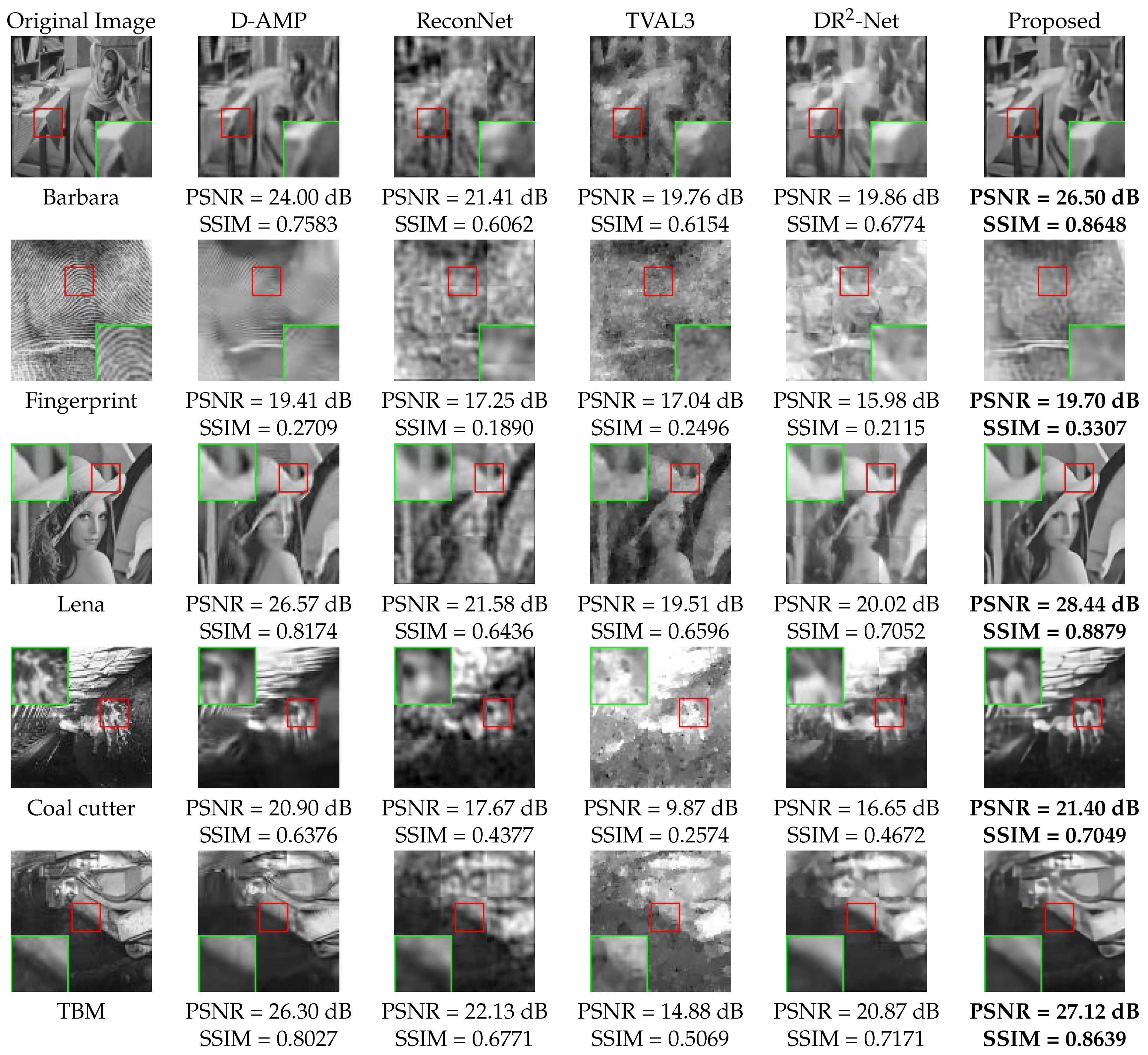
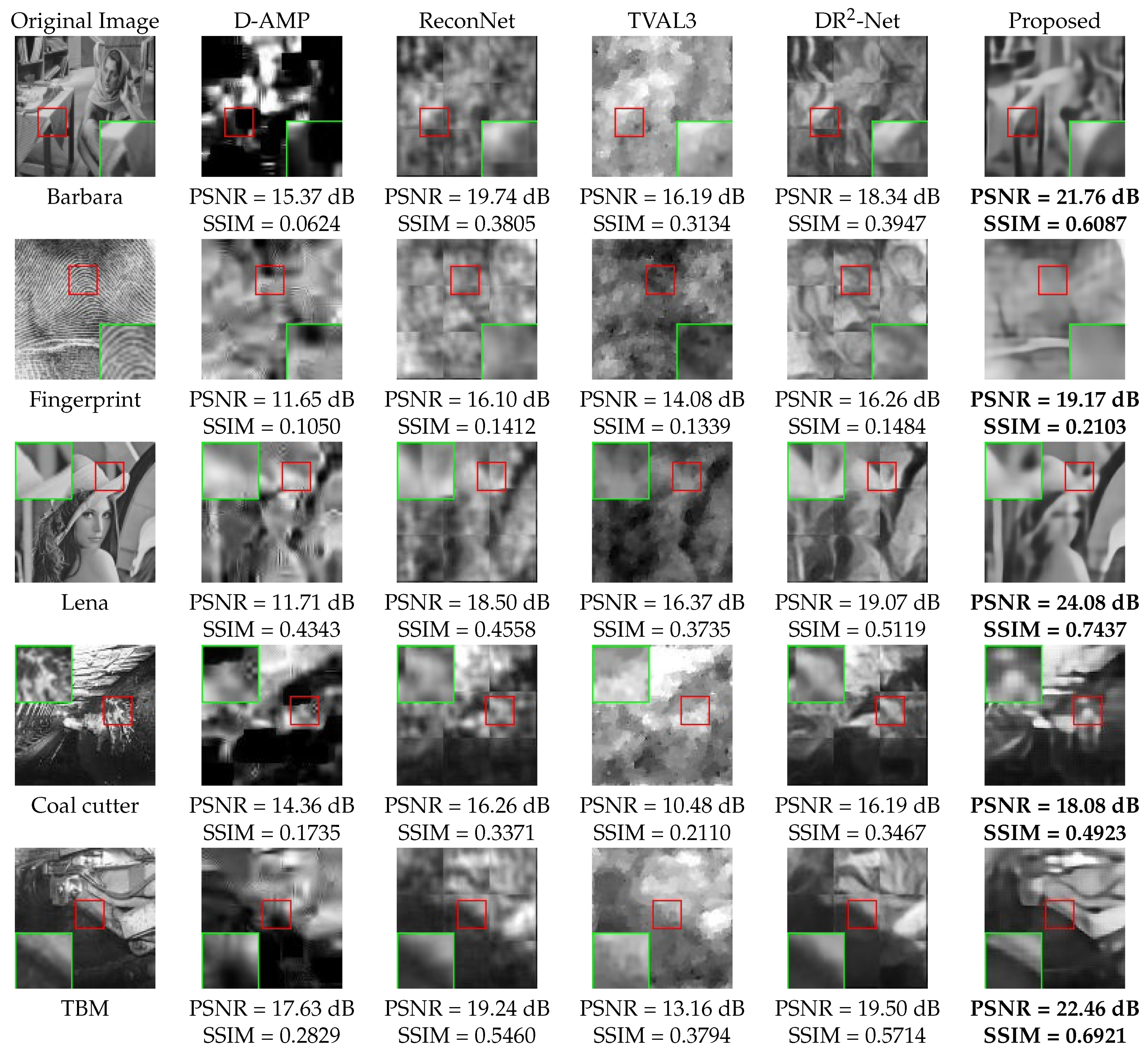
3.3. Visual Quality Evaluation
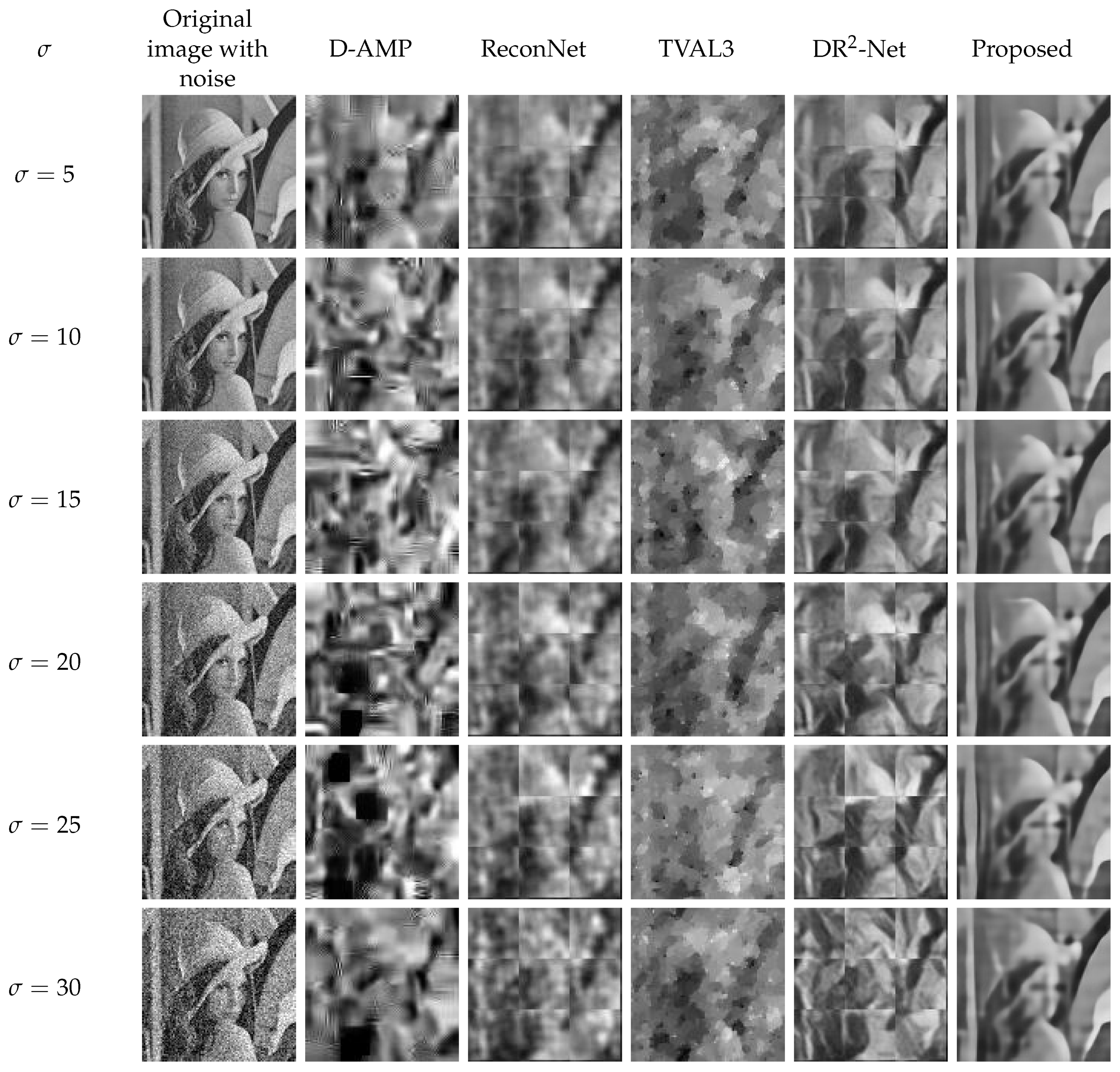
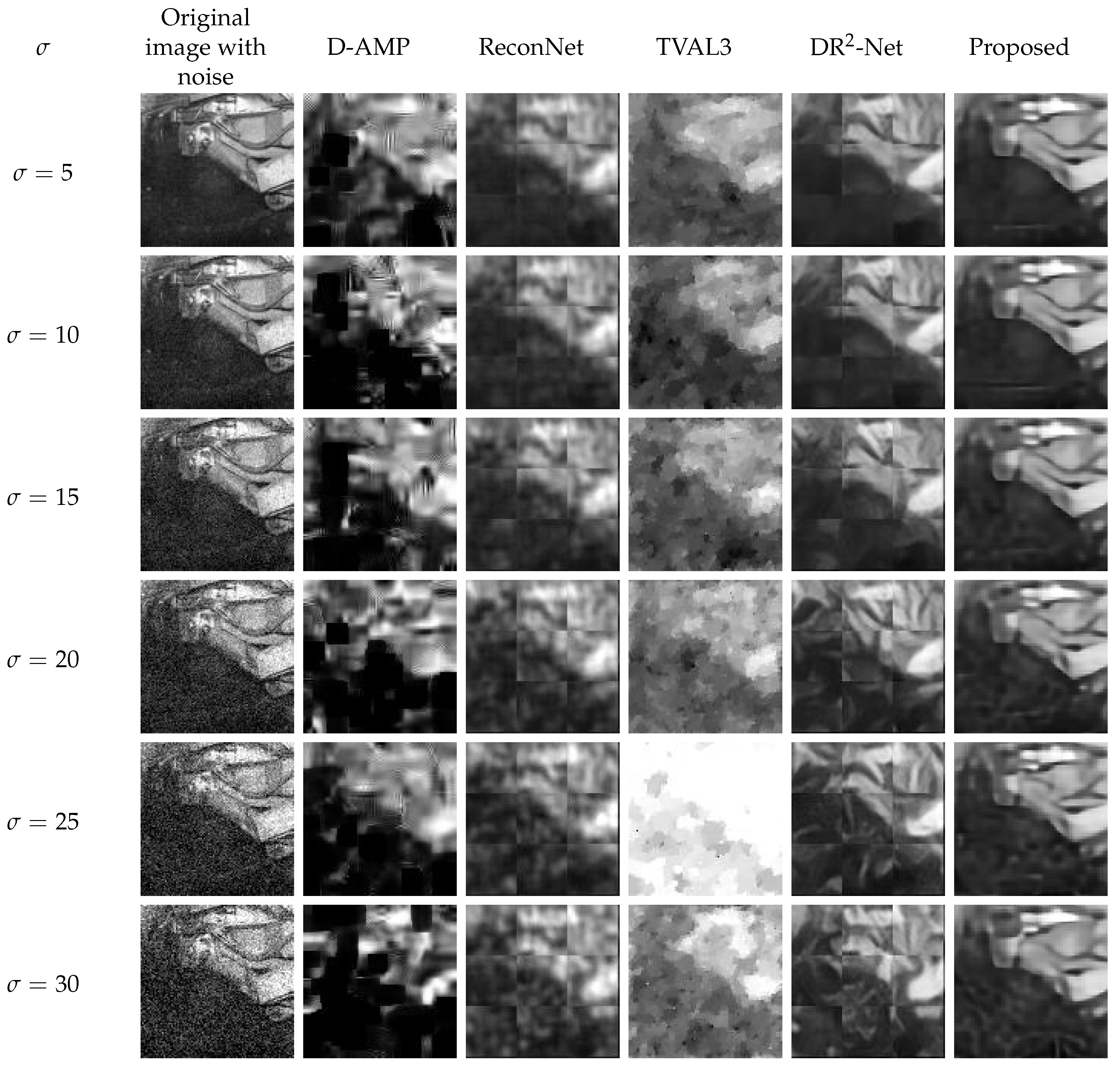
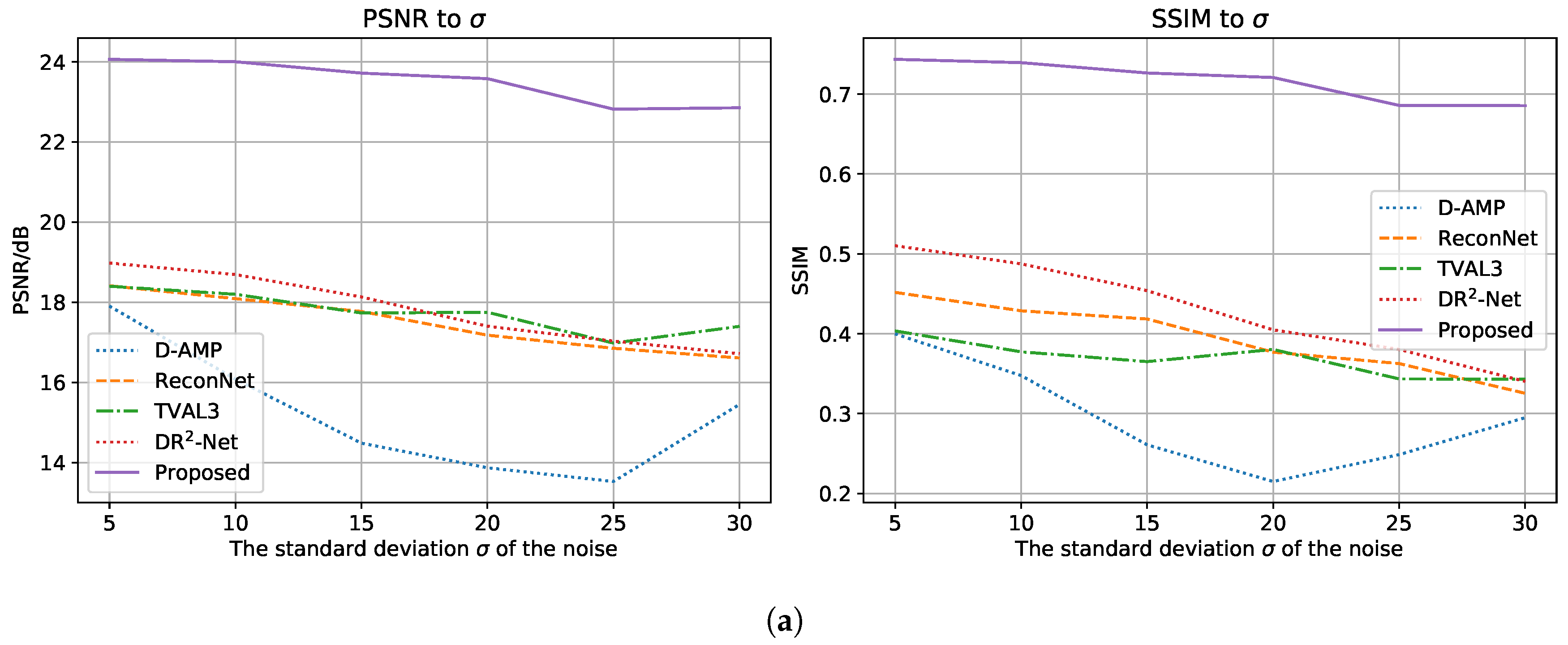
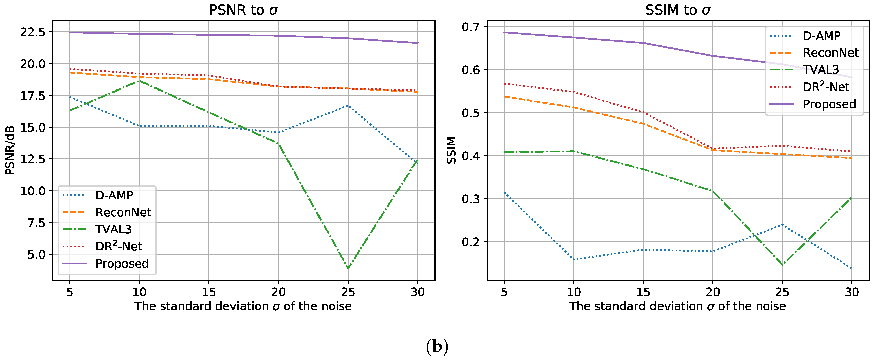
3.4. Robustness against Noise
4. Conclusions
- The proposed method recovers sharp edges in the images. For underground mines, edges in the image are the key component to distinguish the foreground and background. By determining the boundaries of miners and equipment, it is possible for further image analysis to carry out.
- The proposed method features noise robustness. By blurring the dense patterns, the proposed method can filter out the noise especially seen in underground mines.
- Compared to other algorithms, the proposed method excels at low compression ratios. General image compression methods tend to strike a balance between the compression ratio and the recovery quality. They do not have to work at extremely low compression ratios as the transmission bandwidth available is comparably high. However, the proposed method is designed to work at low compression ratios to adapt to the harsh communication environment in underground mines.
Author Contributions
Funding
Conflicts of Interest
References
- Dai, S.; Finkelman, R.B. Coal as a promising source of critical elements: Progress and future prospects. Int. J. Coal Geol. 2018, 186, 155–164. [Google Scholar] [CrossRef]
- Dohare, Y.S.; Maity, T.; Das, P.S.; Paul, P.S. Wireless Communication and Environment Monitoring in Underground Coal Mines- Review. IETE Tech. Rev. 2015, 32, 140–150. [Google Scholar] [CrossRef]
- Wallace, G. The JPEG still picture compression standard. IEEE Trans. Consum. Electron. 1992, 38, xviii–xxxiv. [Google Scholar] [CrossRef]
- Li, M.; Zuo, W.; Gu, S.; Zhao, D.; Zhang, D. Learning Convolutional Networks for Content-Weighted Image Compression. In Proceedings of the 2018 IEEE/CVF Conference on Computer Vision and Pattern Recognition, Salt Lake City, UT, USA, 18–23 June 2018; pp. 3214–3223. [Google Scholar] [CrossRef] [Green Version]
- Marcellin, M.W.; Gormish, M.J.; Bilgin, A.; Boliek, M.P. An overview of JPEG-2000. In Proceedings of the Data Compression Conference (DCC 2000), Snowbird, UT, USA, 28–30 March 2000; pp. 523–541. [Google Scholar] [CrossRef]
- Candes, E.; Romberg, J.; Tao, T. Robust uncertainty principles: Exact signal reconstruction from highly incomplete frequency information. IEEE Trans. Inf. Theory 2006, 52, 489–509. [Google Scholar] [CrossRef] [Green Version]
- Candès, E.J.; Romberg, J.K.; Tao, T. Stable signal recovery from incomplete and inaccurate measurements. Commun. Pure Appl. Math. 2006, 59, 1207–1223. [Google Scholar] [CrossRef] [Green Version]
- Donoho, D.L.; Tanner, J. Thresholds for the Recovery of Sparse Solutions via L1 Minimization. In Proceedings of the IEEE 2006 40th Annual Conference on Information Sciences and Systems, Princeton, NJ, USA, 22–24 March 2006; pp. 202–206. [Google Scholar] [CrossRef]
- Joshi, A.M.; Sahu, C.; Ravikumar, M.; Ansari, S. Hardware implementation of compressive sensing for image compression. In Proceedings of the TENCON 2017—2017 IEEE Region 10 Conference, Penang, Malaysia, 5–8 November 2017; IEEE: Penang, Malaysia, 2017; Volume 2017-Decem, pp. 1309–1314. [Google Scholar] [CrossRef]
- Chambolle, A. An Algorithm for Total Variation Minimization and Applications. J. Math. Imaging Vis. 2004, 20, 89–97. [Google Scholar] [CrossRef]
- Donoho, D.L.; Maleki, A.; Montanari, A. Message-passing algorithms for compressed sensing. Proc. Natl. Acad. Sci. USA 2009, 106, 18914–18919. [Google Scholar] [CrossRef] [Green Version]
- Rudin, L.I.; Osher, S.; Fatemi, E. Nonlinear total variation based noise removal algorithms. Phys. D Nonlinear Phenom. 1992, 60, 259–268. [Google Scholar] [CrossRef]
- Li, C.; Yin, W.; Jiang, H.; Zhang, Y. An efficient augmented Lagrangian method with applications to total variation minimization. Comput. Optim. Appl. 2013, 56, 507–530. [Google Scholar] [CrossRef] [Green Version]
- Kong, Q.; Gong, R.; Liu, J.; Shao, X. Investigation on Reconstruction for Frequency Domain Photoacoustic Imaging via TVAL3 Regularization Algorithm. IEEE Photonics J. 2018, 10, 1–15. [Google Scholar] [CrossRef]
- Metzler, C.A.; Maleki, A.; Baraniuk, R.G. From Denoising to Compressed Sensing. IEEE Trans. Inf. Theory 2016, 62, 5117–5144. [Google Scholar] [CrossRef]
- Zhao, X.; Shen, X.; Wang, K.; Li, W. A DCVS Reconstruction Algorithm for Mine Video Monitoring Image Based on Block Classification. Preprints 2018, 2018070222. [Google Scholar] [CrossRef] [Green Version]
- Wang, Y.; Liu, Z.; Wang, D.; Li, Y.; Yan, J. Anomaly detection and visual perception for landslide monitoring based on a heterogeneous sensor network. IEEE Sens. J. 2017, 17, 1. [Google Scholar] [CrossRef]
- Qiao, X.; Yang, F.; Zheng, J. Ground Penetrating Radar Weak Signals Denoising via Semi-soft Threshold Empirical Wavelet Transform. Ingénierie Des Systèmes d Information 2019, 24, 207–213. [Google Scholar] [CrossRef]
- Xie, S.; Imani, M.; Dougherty, E.R.; Braga-Neto, U.M. Nonstationary linear discriminant analysis. In Proceedings of the IEEE 2017 51st Asilomar Conference on Signals, Systems, and Computers, Pacific Grove, CA, USA, 29 October–1 November 2017; pp. 161–165. [Google Scholar] [CrossRef]
- Imani, M.; Ghoreishi, S.F.; Braga-Neto, U.M. Bayesian control of large MDPs with unknown dynamics in data-poor environments. In Proceedings of the Advances in Neural Information Processing Systems (NIPS), Montréal, QC, Canada, 3–8 December 2018; pp. 8146–8156. [Google Scholar]
- Imani, M.; Ghoreishi, S.F.; Allaire, D.; Braga-Neto, U.M. MFBO-SSM: Multi-Fidelity Bayesian Optimization for Fast Inference in State-Space Models. In Proceedings of the AAAI Conference on Artificial Intelligence, Hilton Hawaiian Village, Honolulu, HI, USA, 27 January 27–1 February 2019; Volume 33, pp. 7858–7865. [Google Scholar] [CrossRef] [Green Version]
- Imani, M.; Dougherty, E.R.; Braga-Neto, U. Boolean Kalman filter and smoother under model uncertainty. Automatica 2020, 111, 108609. [Google Scholar] [CrossRef]
- Ren, S.; He, K.; Girshick, R.; Sun, J. Faster R-CNN: Towards Real-Time Object Detection with Region Proposal Networks. IEEE Trans. Pattern Anal. Mach. Intell. 2017, 39, 1137–1149. [Google Scholar] [CrossRef] [PubMed] [Green Version]
- Redmon, J.; Divvala, S.; Girshick, R.; Farhadi, A. You Only Look Once: Unified, Real-Time Object Detection. In Proceedings of the 2016 IEEE Conference on Computer Vision and Pattern Recognition (CVPR), Las Vegas, NV, USA, 27–30 June 2016; Volume 2016-Decem, pp. 779–788. [Google Scholar] [CrossRef] [Green Version]
- Liu, W.; Anguelov, D.; Erhan, D.; Szegedy, C.; Reed, S.; Fu, C.Y.; Berg, A.C. SSD: Single Shot MultiBox Detector. In Lecture Notes in Computer Science (Including Subseries Lecture Notes in Artificial Intelligence and Lecture Notes in Bioinformatics); Springer International Publishing: Cham, Switzerland, 2016; Volume 9905 LNCS, pp. 21–37. [Google Scholar] [CrossRef] [Green Version]
- Chen, Y.; Zhu, K.; Zhu, L.; He, X.; Ghamisi, P.; Benediktsson, J.A. Automatic Design of Convolutional Neural Network for Hyperspectral Image Classification. IEEE Trans. Geosci. Remote Sens. 2019, 57, 7048–7066. [Google Scholar] [CrossRef]
- Liu, Q.; Feng, C.; Song, Z.; Louis, J.; Zhou, J. Deep Learning Model Comparison for Vision-Based Classification of Full/Empty-Load Trucks in Earthmoving Operations. Appl. Sci. 2019, 9, 4871. [Google Scholar] [CrossRef] [Green Version]
- Mousavi, A.; Baraniuk, R.G. Learning to invert: Signal recovery via Deep Convolutional Networks. In Proceedings of the 2017 IEEE International Conference on Acoustics, Speech and Signal Processing (ICASSP), New Orleans, LA, USA, 5–9 March 2017; pp. 2272–2276. [Google Scholar] [CrossRef] [Green Version]
- Kulkarni, K.; Lohit, S.; Turaga, P.; Kerviche, R.; Ashok, A. ReconNet: Non-Iterative Reconstruction of Images from Compressively Sensed Measurements. In Proceedings of the 2016 IEEE Conference on Computer Vision and Pattern Recognition (CVPR), Las Vegas, NV, USA, 27–30 June 2016; pp. 449–458. [Google Scholar] [CrossRef]
- Yao, H.; Dai, F.; Zhang, S.; Zhang, Y.; Tian, Q.; Xu, C. DR2-Net: Deep Residual Reconstruction Network for image compressive sensing. Neurocomputing 2019, 359, 483–493. [Google Scholar] [CrossRef] [Green Version]
- Ballé, J.; Laparra, V.; Simoncelli, E.P. End-to-end Optimized Image Compression. In Proceedings of the 5th International Conference on Learning Representations, ICLR 2017, Conference Track Proceedings, Toulon, France, 24–26 April 2017. [Google Scholar]
- Wang, C.; Han, Y.; Wang, W. An End-to-End Deep Learning Image Compression Framework Based on Semantic Analysis. Appl. Sci. 2019, 9, 3580. [Google Scholar] [CrossRef] [Green Version]
- Lyu, C.; Liu, Z.; Yu, L. Block-sparsity recovery via recurrent neural network. Signal Process. 2019, 154, 129–135. [Google Scholar] [CrossRef]
- Toderici, G.; Vincent, D.; Johnston, N.; Jin Hwang, S.; Minnen, D.; Shor, J.; Covell, M. Full Resolution Image Compression with Recurrent Neural Networks. In Proceedings of the IEEE Conference on Computer Vision and Pattern Recognition (CVPR), Honolulu, HI, USA, 21–26 July 2017. [Google Scholar]
- Minnen, D.; Toderici, G.; Covell, M.; Chinen, T.; Johnston, N.; Shor, J.; Hwang, S.J.; Vincent, D.; Singh, S. Spatially adaptive image compression using a tiled deep network. In Proceedings of the 2017 IEEE International Conference on Image Processing (ICIP), Beijing, China, 17–20 September 2017; pp. 2796–2800. [Google Scholar] [CrossRef] [Green Version]
- Ma, S.; Zhang, X.; Jia, C.; Zhao, Z.; Wang, S.; Wanga, S. Image and Video Compression with Neural Networks: A Review. IEEE Trans. Circuits Syst. Video Technol. 2019, 8215, 1. [Google Scholar] [CrossRef] [Green Version]
- Rippel, O.; Bourdev, L. Real-time adaptive image compression. In Proceedings of the 34th International Conference on Machine Learning, ICML 2017, Sydney, Australia, 6–11 August 2017; Volume 6, pp. 4457–4473. [Google Scholar]
- Jia, C.; Zhang, X.; Wang, S.; Wang, S.; Ma, S. Light Field Image Compression Using Generative Adversarial Network-Based View Synthesis. IEEE J. Emerg. Sel. Top. Circuits Syst. 2019, 9, 177–189. [Google Scholar] [CrossRef]
- Bjontegaard, G. Calculation of average PSNR differences between RD-curves. In Proceedings of the VCEG Meeting (ITU-T SG16 Q.6), Austin, TX, USA, 2–4 April 2001; pp. 2–4. [Google Scholar]
- Agustsson, E.; Tschannen, M.; Mentzer, F.; Timofte, R.; Gool, L.V. Generative Adversarial Networks for Extreme Learned Image Compression. In Proceedings of the IEEE International Conference on Computer Vision (ICCV), Seoul, Korea, 27 October–2 November 2019. [Google Scholar]
- He, K.; Zhang, X.; Ren, S.; Sun, J. Delving Deep into Rectifiers: Surpassing Human-Level Performance on ImageNet Classification. In Proceedings of the 2015 IEEE International Conference on Computer Vision (ICCV), Santiago, Chile, 7–13 December 2015; pp. 1026–1034. [Google Scholar] [CrossRef] [Green Version]
- Miklós, P. Image interpolation techniques. In Proceedings of the 2nd Siberian-Hungarian Joint Symposium On Intelligent Systems, Subotica, Serbia and Montenegro, 1–2 October 2004; pp. 1–6. [Google Scholar]
- Ioffe, S.; Szegedy, C. Batch Normalization: Accelerating Deep Network Training by Reducing Internal Covariate Shift. In Proceedings of the 32nd International Conference on Machine Learning, ICML 2015, Lille, France, 6–11 July 2015; Volume 1, pp. 448–456. [Google Scholar]
- He, K.; Zhang, X.; Ren, S.; Sun, J. Deep Residual Learning for Image Recognition. In Proceedings of the 2016 IEEE Conference on Computer Vision and Pattern Recognition (CVPR), Las Vegas, NV, USA, 27–30 June 2016; pp. 770–778. [Google Scholar] [CrossRef] [Green Version]
- Maas, A.L.; Hannun, A.Y.; Ng, A.Y. Rectifier nonlinearities improve neural network acoustic models. In Proceedings of the ICML Workshop on Deep Learning for Audio, Speech and Language Processing, Atlanta, GA, USA, 16 June 2013. [Google Scholar]
- Wang, Z.; Bovik, A.C. Mean squared error: Love it or leave it? A new look at Signal Fidelity Measures. IEEE Signal Process. Mag. 2009, 26, 98–117. [Google Scholar] [CrossRef]
- Wang, Z.; Bovik, A.C.; Sheikh, H.R.; Simoncelli, E.P. Image quality assessment: From error visibility to structural similarity. IEEE Trans. Image Process. 2004, 13, 600–612. [Google Scholar] [CrossRef] [Green Version]
- Sampat, M.P.; Wang, Z.; Gupta, S.; Bovik, A.C.; Markey, M.K. Complex Wavelet Structural Similarity: A New Image Similarity Index. IEEE Trans. Image Process. 2009, 18, 2385–2401. [Google Scholar] [CrossRef]
- Mallat, S.G. A theory for multiresolution signal decomposition: The wavelet representation. IEEE Trans. Pattern Anal. Mach. Intell. 1989, 11, 674–693. [Google Scholar] [CrossRef] [Green Version]
- Kotu, V.; Deshpande, B. Classification. In Data Science; Elsevier: Amsterdam, The Netherlands, 2019; pp. 65–163. [Google Scholar] [CrossRef]
- Kingma, D.P.; Ba, J.L. Adam: A method for stochastic optimization. In Proceedings of the 3rd International Conference on Learning Representations, ICLR 2015 - Conference Track Proceedings, San Diego, CA, USA, 7–9 May 2015. [Google Scholar]
- Lin, T.Y.; Maire, M.; Belongie, S.; Bourdev, L.; Girshick, R.; Hays, J.; Perona, P.; Ramanan, D.; Zitnick, C.L.; Dollár, P. Microsoft COCO: Common Objects in Context. In Computer Vision—ECCV 2014; Springer International Publishing: Cham, Switzerland, 2014; Volume 8693 LNCS, pp. 740–755. [Google Scholar] [CrossRef] [Green Version]
- Paszke, A.; Chintala, S.; Chanan, G.; Lin, Z.; Gross, S.; Yang, E.; Antiga, L.; Devito, Z.; Lerer, A.; Desmaison, A. Automatic differentiation in PyTorch. In Proceedings of the 31st Conference on Neural Information Processing Systems, Long Beach, CA, USA, 4–9 December 2017. [Google Scholar]


| Image | Algorithm | r = 0.25 | r = 0.20 | r = 0.15 | r = 0.10 | r = 0.04 | r = 0.01 |
|---|---|---|---|---|---|---|---|
| Barbara | D-AMP | 26.61 | 25.37 | 24.00 | 21.73 | 15.37 | 7.23 |
| ReconNet | 25.14 | 22.80 | 21.41 | 21.79 | 19.74 | 16.20 | |
| TVAL3 | 22.40 | 21.28 | 19.76 | 18.87 | 16.19 | 15.15 | |
| DR-Net | 25.43 | 21.64 | 19.86 | 20.99 | 18.34 | 16.08 | |
| Proposed | 27.23 | 27.62 | 26.50 | 24.15 | 21.76 | 17.86 | |
| Fingerprint | D-AMP | 20.99 | 20.64 | 19.41 | 19.07 | 11.65 | 5.24 |
| ReconNet | 17.56 | 17.20 | 17.25 | 16.68 | 16.10 | 15.55 | |
| TVAL3 | 18.25 | 17.45 | 17.04 | 15.57 | 14.08 | 9.68 | |
| DR-Net | 18.30 | 16.57 | 15.98 | 17.16 | 16.26 | 15.20 | |
| Proposed | 19.76 | 19.80 | 19.70 | 19.39 | 19.17 | 18.68 | |
| Lena | D-AMP | 30.28 | 28.40 | 26.57 | 24.38 | 11.71 | 6.57 |
| ReconNet | 23.83 | 22.65 | 21.58 | 20.32 | 18.50 | 15.90 | |
| TVAL3 | 21.26 | 20.68 | 19.51 | 17.81 | 16.37 | 15.17 | |
| DR-Net | 26.37 | 21.93 | 20.02 | 21.82 | 19.07 | 15.77 | |
| Proposed | 28.82 | 29.01 | 28.44 | 25.48 | 24.08 | 19.47 | |
| Coal cutter | D-AMP | 21.81 | 21.86 | 20.90 | 19.10 | 14.36 | 8.14 |
| ReconNet | 18.78 | 18.35 | 17.67 | 17.24 | 16.26 | 14.52 | |
| TVAL3 | 12.52 | 10.94 | 9.87 | 8.17 | 10.48 | 12.50 | |
| DR-Net | 20.22 | 17.71 | 16.65 | 17.76 | 16.19 | 14.78 | |
| Proposed | 21.78 | 21.84 | 21.40 | 20.05 | 18.08 | 17.34 | |
| TBM | D-AMP | 29.68 | 28.02 | 26.30 | 24.51 | 17.63 | 8.76 |
| ReconNet | 23.89 | 22.95 | 22.13 | 21.21 | 19.24 | 17.65 | |
| TVAL3 | 17.27 | 16.17 | 14.88 | 14.35 | 13.16 | 13.71 | |
| DR-Net | 25.65 | 22.11 | 20.87 | 22.04 | 19.50 | 17.53 | |
| Proposed | 27.67 | 27.27 | 27.12 | 24.95 | 22.46 | 20.03 |
| Image | Algorithm | r = 0.25 | r = 0.20 | r = 0.15 | r = 0.10 | r = 0.04 | r = 0.01 |
|---|---|---|---|---|---|---|---|
| Barbara | D-AMP | 0.8570 | 0.7781 | 0.7583 | 0.6189 | 0.0624 | 0.0129 |
| ReconNet | 0.7449 | 0.7037 | 0.6062 | 0.5506 | 0.3805 | 0.2226 | |
| TVAL3 | 0.7391 | 0.6834 | 0.6154 | 0.4692 | 0.3134 | 0.2281 | |
| DR-Net | 0.8165 | 0.7396 | 0.6774 | 0.6137 | 0.3947 | 0.2283 | |
| Proposed | 0.8823 | 0.8950 | 0.8648 | 0.7832 | 0.6087 | 0.2859 | |
| Fingerprint | D-AMP | 0.5530 | 0.4063 | 0.2709 | 0.2288 | 0.1050 | 0.0029 |
| ReconNet | 0.2438 | 0.2245 | 0.1890 | 0.1871 | 0.1412 | 0.0970 | |
| TVAL3 | 0.3448 | 0.2884 | 0.2496 | 0.1948 | 0.1339 | 0.0774 | |
| DR-Net | 0.3030 | 0.2291 | 0.2115 | 0.2044 | 0.1484 | 0.0976 | |
| Proposed | 0.3464 | 0.3742 | 0.3307 | 0.2871 | 0.2103 | 0.1498 | |
| Lena | D-AMP | 0.8867 | 0.8667 | 0.8174 | 0.7550 | 0.4343 | 0.0235 |
| ReconNet | 0.7412 | 0.7084 | 0.6436 | 0.5997 | 0.4558 | 0.3181 | |
| TVAL3 | 0.7420 | 0.7145 | 0.6596 | 0.5370 | 0.3735 | 0.2869 | |
| DR-Net | 0.8200 | 0.7771 | 0.7052 | 0.6597 | 0.5119 | 0.3352 | |
| Proposed | 0.8930 | 0.9040 | 0.8879 | 0.8301 | 0.7437 | 0.4440 | |
| Coal cutter | D-AMP | 0.6854 | 0.6793 | 0.6376 | 0.5148 | 0.1735 | 0.0363 |
| ReconNet | 0.5470 | 0.4947 | 0.4377 | 0.4267 | 0.3371 | 0.2431 | |
| TVAL3 | 0.3830 | 0.3146 | 0.2574 | 0.1838 | 0.2110 | 0.1608 | |
| DR-Net | 0.6358 | 0.5482 | 0.4672 | 0.4899 | 0.3467 | 0.2634 | |
| Proposed | 0.7320 | 0.7476 | 0.7049 | 0.6303 | 0.4923 | 0.3498 | |
| TBM | D-AMP | 0.8711 | 0.6793 | 0.8027 | 0.7187 | 0.2829 | 0.0634 |
| ReconNet | 0.7728 | 0.7319 | 0.6771 | 0.6522 | 0.5460 | 0.4318 | |
| TVAL3 | 0.5445 | 0.4868 | 0.5069 | 0.4127 | 0.3794 | 0.3372 | |
| DR-Net | 0.8184 | 0.7523 | 0.7171 | 0.6755 | 0.5714 | 0.4456 | |
| Proposed | 0.8793 | 0.8764 | 0.8639 | 0.8058 | 0.6921 | 0.5359 |
© 2019 by the authors. Licensee MDPI, Basel, Switzerland. This article is an open access article distributed under the terms and conditions of the Creative Commons Attribution (CC BY) license (http://creativecommons.org/licenses/by/4.0/).
Share and Cite
Zhang, F.; Xu, Z.; Chen, W.; Zhang, Z.; Zhong, H.; Luan, J.; Li, C. An Image Compression Method for Video Surveillance System in Underground Mines Based on Residual Networks and Discrete Wavelet Transform. Electronics 2019, 8, 1559. https://0-doi-org.brum.beds.ac.uk/10.3390/electronics8121559
Zhang F, Xu Z, Chen W, Zhang Z, Zhong H, Luan J, Li C. An Image Compression Method for Video Surveillance System in Underground Mines Based on Residual Networks and Discrete Wavelet Transform. Electronics. 2019; 8(12):1559. https://0-doi-org.brum.beds.ac.uk/10.3390/electronics8121559
Chicago/Turabian StyleZhang, Fan, Zhichao Xu, Wei Chen, Zizhe Zhang, Hao Zhong, Jiaxing Luan, and Chuang Li. 2019. "An Image Compression Method for Video Surveillance System in Underground Mines Based on Residual Networks and Discrete Wavelet Transform" Electronics 8, no. 12: 1559. https://0-doi-org.brum.beds.ac.uk/10.3390/electronics8121559