1. Introduction
In this paper, we present a fully integratable implementation form of the fractional-order controllers and their application to the DC motor control and two-tank system, respectively, using a non-integer calculus technique.
The transfer function of a fractional-order proportional-integral-derivative (PI
D
) controller, with
being the orders of integration and differentiation, is the following:
where
is the proportional gain,
is the integration constant,
is the differentiation constant, and
are the orders of integration and differentiation, respectively [
1].
Inspecting (
1), it is readily obtained that PI
D
controllers have five parameters, instead of three parameters offered by their integer-order counterparts (i.e., PID controllers), making them very attractive from the implementation point of view [
2]. It must be mentioned at this point that there are many fractional-order controllers/compensators, as for example [
3]: fractional-order controller in traditional PID structure, CRONE controller, TID compensator, lead-lag compensator, and so on.
Due to the absence of commercially available fractional-order capacitors [
4,
5], it is difficult to implement fractional-order controllers through the substitution of conventional capacitors by fractional-order capacitors. Therefore, the implementation of fractional-order controllers can be performed through the utilization of RC networks [
6,
7,
8,
9,
10,
11,
12,
13,
14,
15], which approximate the behavior of the fractional-order capacitors. This is an easy design procedure, but the absence of tunability of the characteristics of the approximated fractional-order capacitors limits its employment only in cases where elements with pre-defined characteristics are required [
7,
10]. Another way for implementing fractional-order controllers is through the approximation of the transfer functions of the required fractional-order differentiation and/or integration stages. This is performed by expressing these transfer functions as rational integer-order transfer functions, which are then implemented using multi-feedback structures [
16].
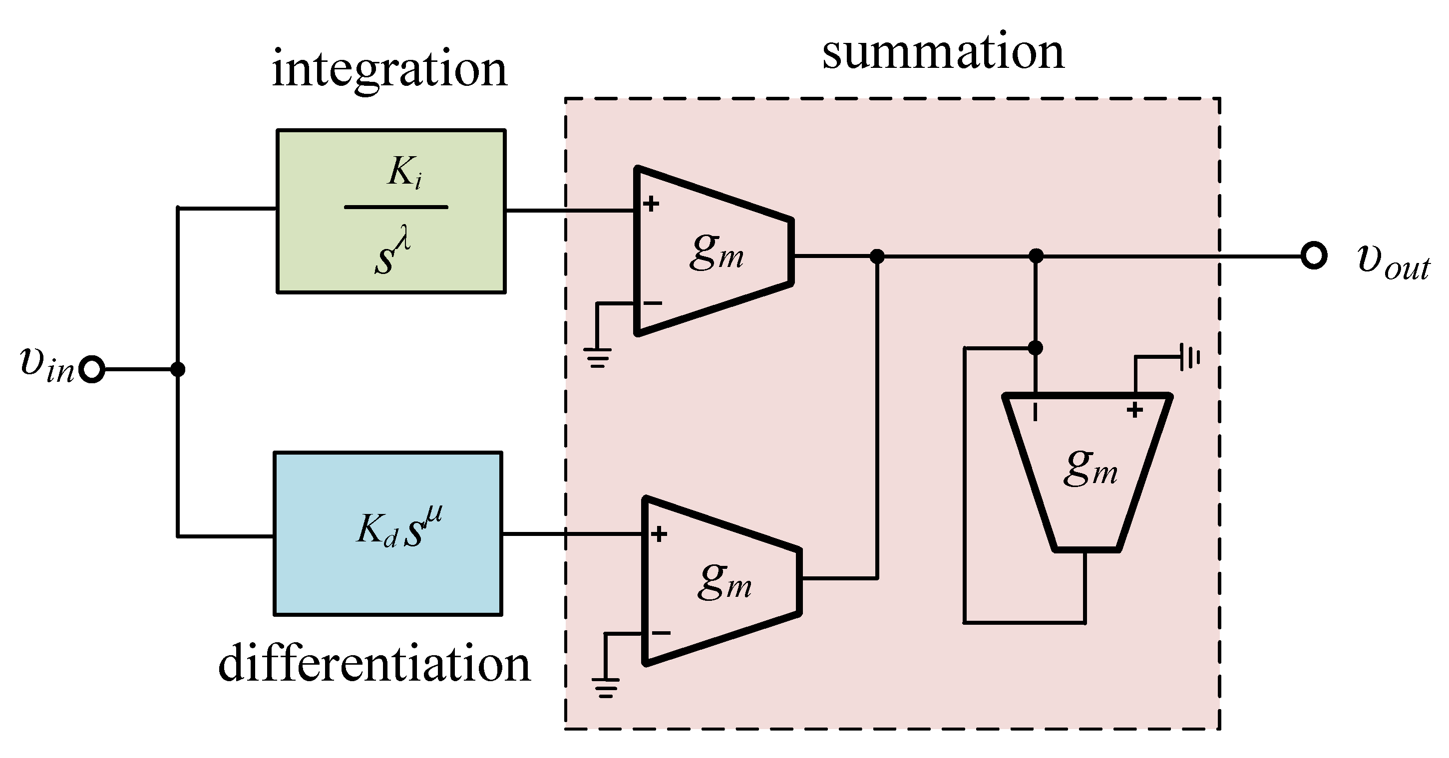
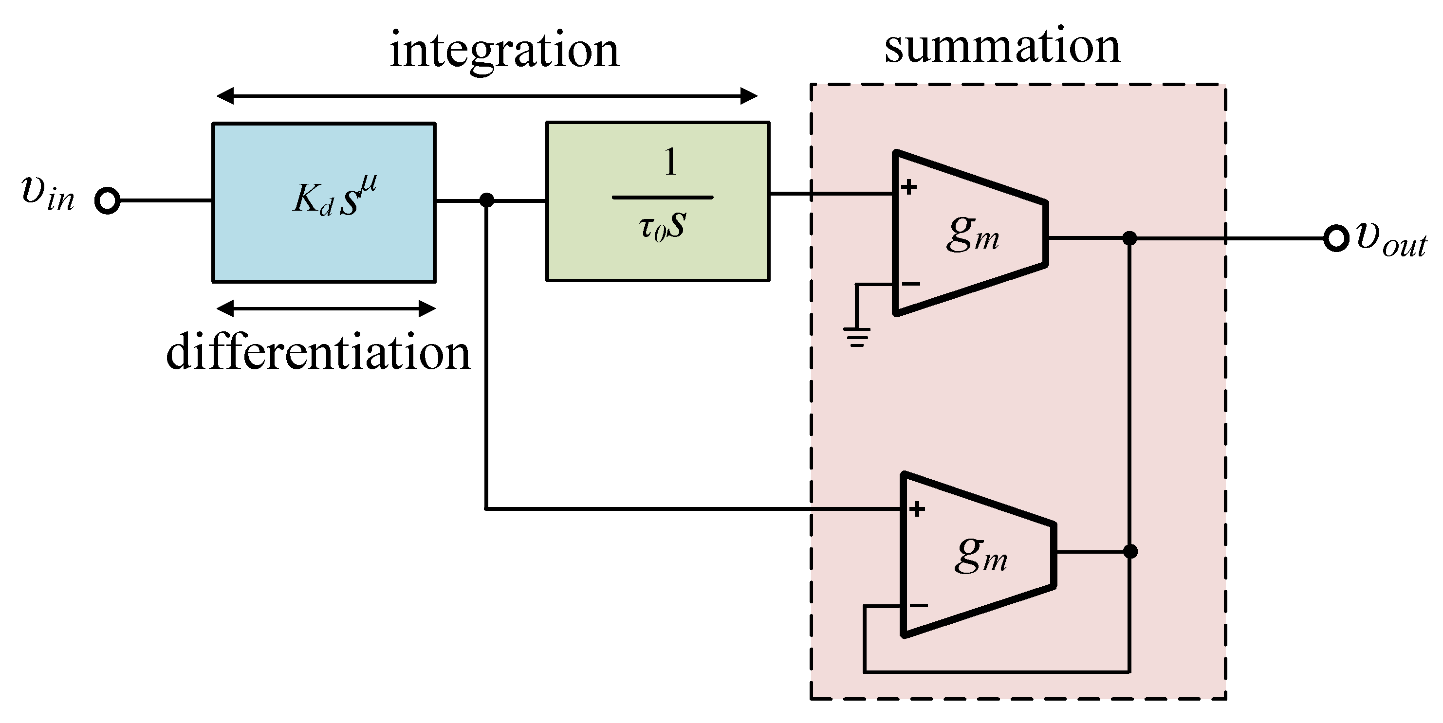
DC motor is a power actuator, which converts direct current electrical energy into rotational mechanical energy. The DC motors are still often used in industry and in numerous control applications, robotic manipulators and commercial applications such as disk drive, tape motor as well. Considering an armature-controlled DC motor in which a constant field current is been utilized, a fractional-order I
D
controller for controlling the rotation speed has been developed in [
17], which offers resistorless implementation, electronic tunability, and capability of monolithic implementation. All these features are originated from the employment of Operational Transconductance Amplifiers (OTAs) as active elements. On the other hand, the active component count and, therefore, the power consumption, are relatively high in this implementation. Owing to the fact that increased number of active elements means increased power dissipation, the reduction of the active component count is very important in nowadays applications, where there is demand for reduced power systems. In order to overcome the aforementioned obstacle, a novel I
D
controller topology is introduced in this work, where the most attractive achievement is that the number of active elements is significantly reduced. This is achieved by expressing the transfer function of the fractional-order integrator as a product of the transfer functions of a fractional-order differentiator and an integer-order integrator. In addition, the proposed structure still offers the benefit of the electronic adjustment of its characteristics and this is very important because possible deviations in frequency characteristics caused by the imperfections of the employed active cells can be easily minimized through appropriate adjustment of the corresponding dc bias currents.
The control of liquid level in tanks as well as its flow between tanks is a very important problem in industry. This is originated from the fact that most of industrial application of liquid level control is hazardous in chemical petroleum, mixing treatment industries, pharmaceutical and food processing industries. Therefore, the development of the corresponding controllers has a significant practical value. Towards this goal, a novel PI controller suitable for controlling the liquid level into a two tank system is introduced, where the employed active blocks for implementing the required fractional-order integrator were current-mirrors, while the gain stage was implemented by a simple trans-linear loop. The resulting benefit is that the transistor count is minimized and, consequently, the dc power consumption is minimized. Originating from the electronic tuning capability of the controller, the same core can be used for implementing controllers with different characteristics, providing design versatility and flexibility.
This article is organized as follows: the proposed fractional-order DC motor controller design is presented and evaluated in
Section 2. In
Section 3, an example of control of two interactive tanks system, new controller topology, and simulation results are presented.
Section 4 concludes this article with some ideas for further work.
3. Proposed Fractional-Order Controller of Two Interactive Tanks
Following the previous example, where OTAs have been employed as active elements in order to implement a fractional-order DC motor ID controller, in this example a new concept is presented. Although OTAs approach offers electronic tunability through appropriate reconfiguration of the biasing DC currents or voltages in the circuit, its disadvantage is the increased number of necessary transistors leading to an increase in power dissipation.
In order to overcome the aforementioned obstacles, a novel fractional-order proportional-integral (PI
) controller topology is introduced in this example with the attractive features: (a) reduced number of MOS transistors compared to that required in [
17] and (b) electronic tuning capability of both proportional gain and integration constant. Electronic tuning of the proportional gain is achieved through the utilization of the trans-linear circuit design principle for implementing a programmable gain stage, while the tuning of the integration constant is achieved through the employment of biasing currents. The designed controller is suitable for controlling, for example, the liquid level into two interacting tank system where the adjustment of the controller parameters for different operating conditions is performed without altering the core of the controller, simply by adjusting the appropriate electrical bias currents.
3.1. Description of the Controller
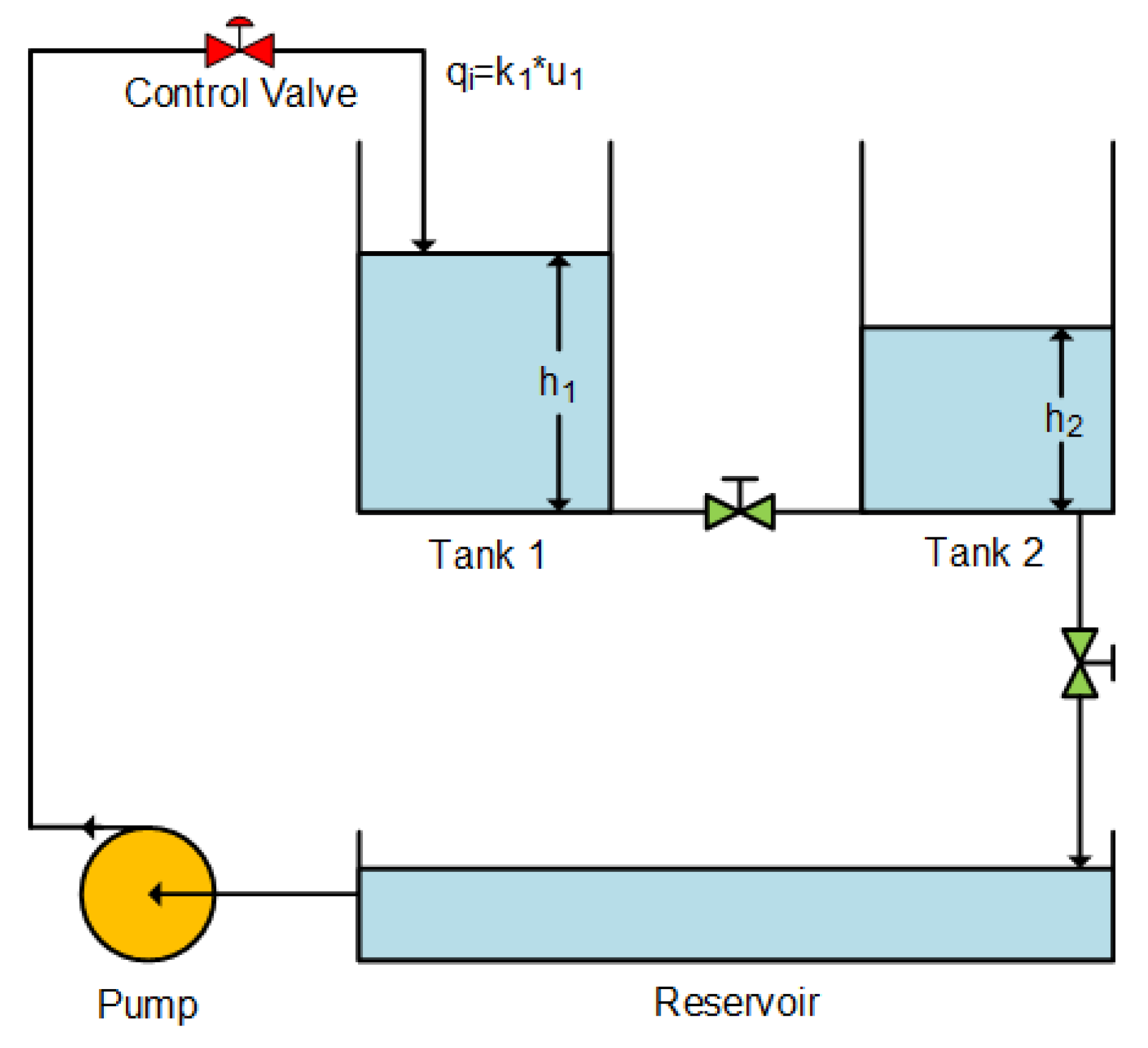
The two interacting tank system is used in many industrial processes, like petroleum refineries, the paper industry and water treatment facilities. The main problem in these processes is the control of liquid level in tank system and flow between tanks, which varies among different systems. The shape, volume and area of the tanks, the inflow and outflow rate, the type of liquid and the ambient conditions are factors that affect the whole operation of the system and, thus, the required control.
A two interacting tank level system is demonstrated in
Figure 10 (adopted from [
23]). It consists of two identical cylindrical tanks, with equal cross sectional area, which are connected through cylindrical pipes of uniform cross sectional area. The liquid is pumped from the reservoir into the first tank through a control valve, while the two tanks are interconnected through manual valves. The objective is to control the level of liquid in tank 2 by varying the inflow rate (
) in tank 1. In this work, we consider five different operating points, determined by the height in tank 1 (
) and in tank 2 (
) as given in
Table 2. The corresponding transfer functions
(
) of the controller are, respectively:
Inspecting (
11)–(
15), it is concluded that only the proportional gain and integration constant change while the order of integration
remains constant. This is very important because if we consider that the transfer function of an integrator of order
has the general form
where
is the associated time-constant, then the integration constant
and the time-constant are related as
Utilizing a fractional-order capacitor with pseudo-capacitance
(expressed in
) and the small-signal transconductance
(measured in
) of a MOS transistor for realizing the required time-constant, then the expression in (
17) can be alternatively written as
Substituting (
18) into (
17) one obtains
The transconductance of a MOS transistor operating in the sub-threshold region is known to be given by
where
is a DC bias current. Therefore, using (
19) and (
20) we obtain
which means that the tuning of the integration constant could be performed through the appropriate linearly adjusted DC bias current, avoiding the requirement for tuning the value of the fractional-order capacitor. This means that a fixed RC network can be used to approximate the behavior of
.
3.2. Controller Building Blocks
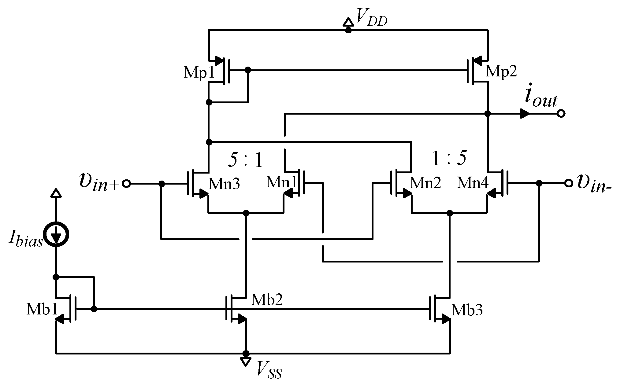
3.2.1. Proportional Stage
The implementation of a gain stage can be easily performed using the simple current-mirror topology depicted in
Figure 11a, where the aspect ratio of transistor Mn2 is
times the aspect ratio of the diode-connected transistor Mn1 [
24]. The input-output relationship, which is realized by the circuit in
Figure 11a, is:
. Although this topology offers simple circuitry, it suffers from the absence of electronic adjustment of the gain. This is due to the fact that the scaling factor
is tuned through the geometry of the corresponding MOS transistors. Although a bank of output branches of the current-mirror in
Figure 11a could be established, which will be digitally controlled, only pre-defined values of the gain are possible, losing the benefit of the design versatility.
In order to overcome this obstacle, the topology depicted in
Figure 11b will be employed. Assuming that transistors Mp1-Mp4 are identical and are biased in the sub-threshold region, then by applying the trans-linear principle [
25] in the loop formed by Mp1-Mp4, it is derived that
Since
,
,
, and
, the expression of the output current, obtained after some algebraic manipulation, is
Thus, the gain is now electronically adjusted through the ratio of the DC bias currents and without altering the aspect ratio of the MOS transistors.
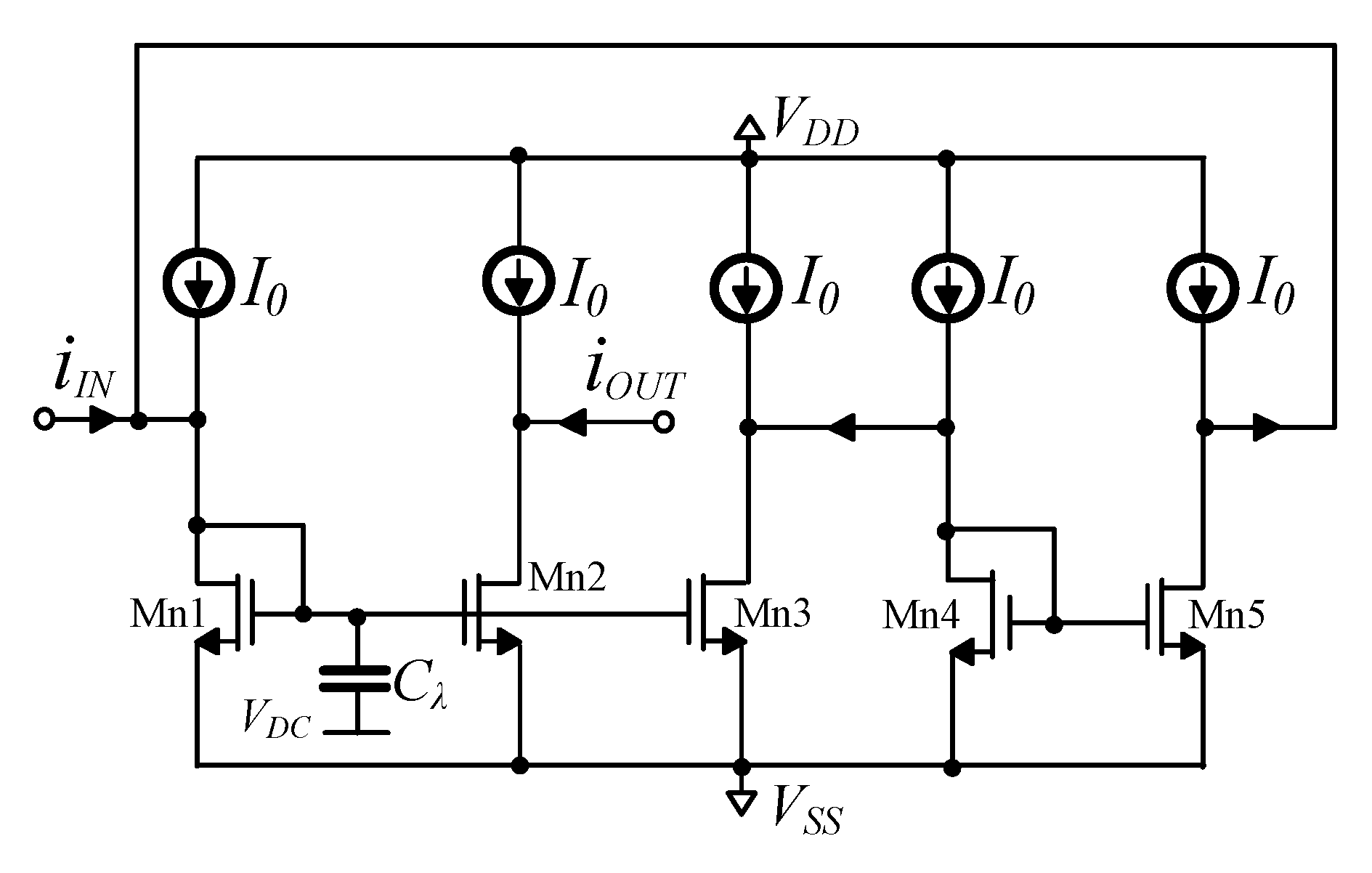
3.2.2. Integration Stage
The topology of a fractional-order lossless integrator, using current-mirrors, is depicted in
Figure 12. The impedance of the fractional-order capacitor
is given by (
24)
and the realized transfer function is
with
being the transconductance parameter of the diode-connected transistor Mn1, calculated using the formula in (
20). Comparing (
16) and (
25), it is easily obtained that the realized time-constant is given by the form of (
18) and, consequently, the expression in (
21) is still valid.
A practical problem that appears, for a given value of the pseudo-capacitance
, is that the values of the DC bias current
could be relatively high. This is due to the fact that according to (
11)–(
15), the maximum current will be 60 times the basic current. For example, considering that
, the calculated maximum value will be equal to 0.6
. In order to overcome this problem, the integration stage in
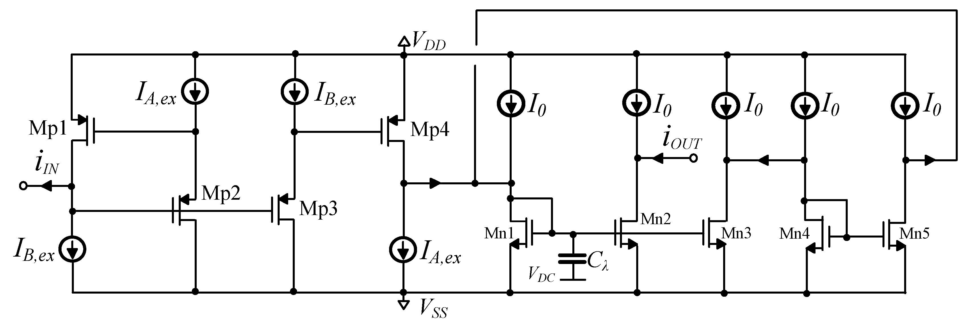
Figure 12 will be enhanced by embedding a topology similar to that in
Figure 11b, as it is demonstrated in
Figure 13. As a result, the integration constant becomes
with the gain factor given by the formula:
. Considering a fractional-order capacitor equal to
and considering
, then according to (
26), the relationship between the proportional and integration constant becomes
and, consequently, the set of values of
that must be implemented are {
}. Taking into account that these values are determined by the ratio of the appropriate DC currents, it is obvious that this extra degree of freedom offers reasonable values of currents, in order to keep the transistors operating in the sub-threshold region. The price paid is the increased circuit complexity of the integrator.
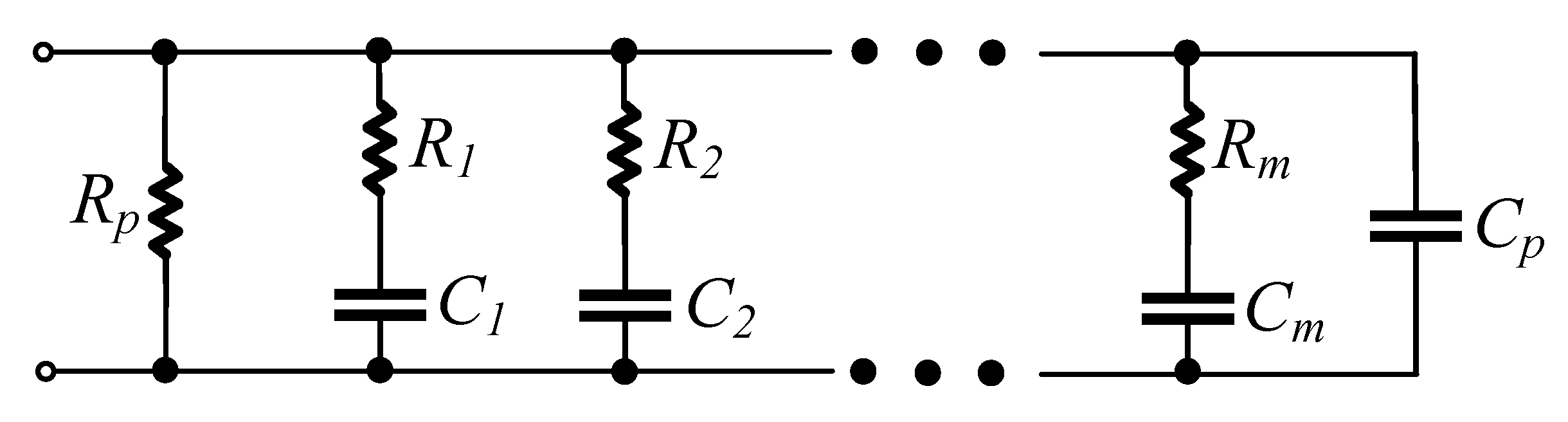
3.2.3. Fractional-Order Capacitor Emulator
An efficient network for approximating the behavior of a fractional-order capacitor is demonstrated in
Figure 14, constructed from
m parallel RC branches and two correction elements notated as
and
, respectively [
26]. The total admittance of this network is given by (
27)
Given the pseudo-capacitance
, the fractional order
, the phase error
within the frequency range [
], then choosing the values of
and
in such a way that the
, the values of passive elements are calculated through the formula
The factors
are derived through (
30) and (
31)
Calculating the impedance
at the average frequency
from (
27) and comparing the achieved result with the theoretically predicted value, which is equal to
, the values of all the resistors must be multiplied while all the capacitances must be divided by the same factor in order to appropriately scale the implemented impedance. Another point that must be mentioned is that the number of required sections is calculated according to (
32), rounded to the nearest integer
Following the procedure described in
Section 3.2.3, the values of passive elements for approximating a fractional-order capacitor of order
and pseudo-capacitance
with phase error
within the frequency range [
] derived using the Matlab code available in [
27], are summarized in
Table 3. The magnitude and phase responses along with the theoretically predicted ones, which are given by dashes, are plotted in
Figure 15a,b, respectively. The phase response, which is very important for the simulation of the fractional-order capacitor, is also very close to the ideal value of
, with the defined expected maximum error of
for almost the entire frequency band. The error is increased for frequencies higher than 2 Hz and reaches a maximum of
at 10 Hz.
3.3. Simulation Results
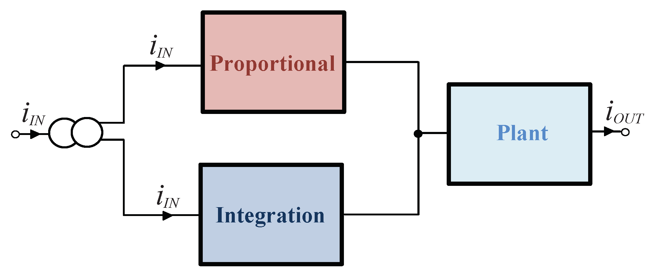
The functional block diagram of the realized controller is provided in
Figure 16, where the plant is described by the transfer functions
, which correspond to the five different operating points described in
Table 2.
In order to evaluate the behavior of the controller, the same CMOS process will be used as in the previous design example. The employed DC bias voltage scheme was .
With regards to the gain stage in
Figure 11b, the DC current
has been chosen equal to 200 pA. Using (
11)–(
15) the calculated values of the DC bias current
were
pA. The dimensions of transistors Mp1-Mp4 were
, while the distribution of the DC bias current
has been performed using current-mirrors with the aspect ratio of the nMOS and pMOS transistors equal to
and
, respectively. In the case of the substitution of the DC bias current
, the corresponding values were
and
. The bias current
of the integrators has been chosen equal to 9 nA. Considering a
pseudo-capacitance then, using (
26) and choosing
pA, the values of
have been calculated as
nA. The aspect ratio of transistors Mp1–Mp4 in
Figure 13 were
and the aspect ratios of the transistors in the current mirrors used for distributing the currents
and
were
,
, and
,
, respectively. The aspect ratio of transistors Mn1–Mn5 in
Figure 13 was
and the distribution of the DC bias current
has been performed using current-mirrors with transistor aspect ratio
. Finally, the distribution of the input current of the controller was also performed using current-mirrors with transistor aspect ratios equal to
. The DC bias current of this stage was equal to 200 pA.
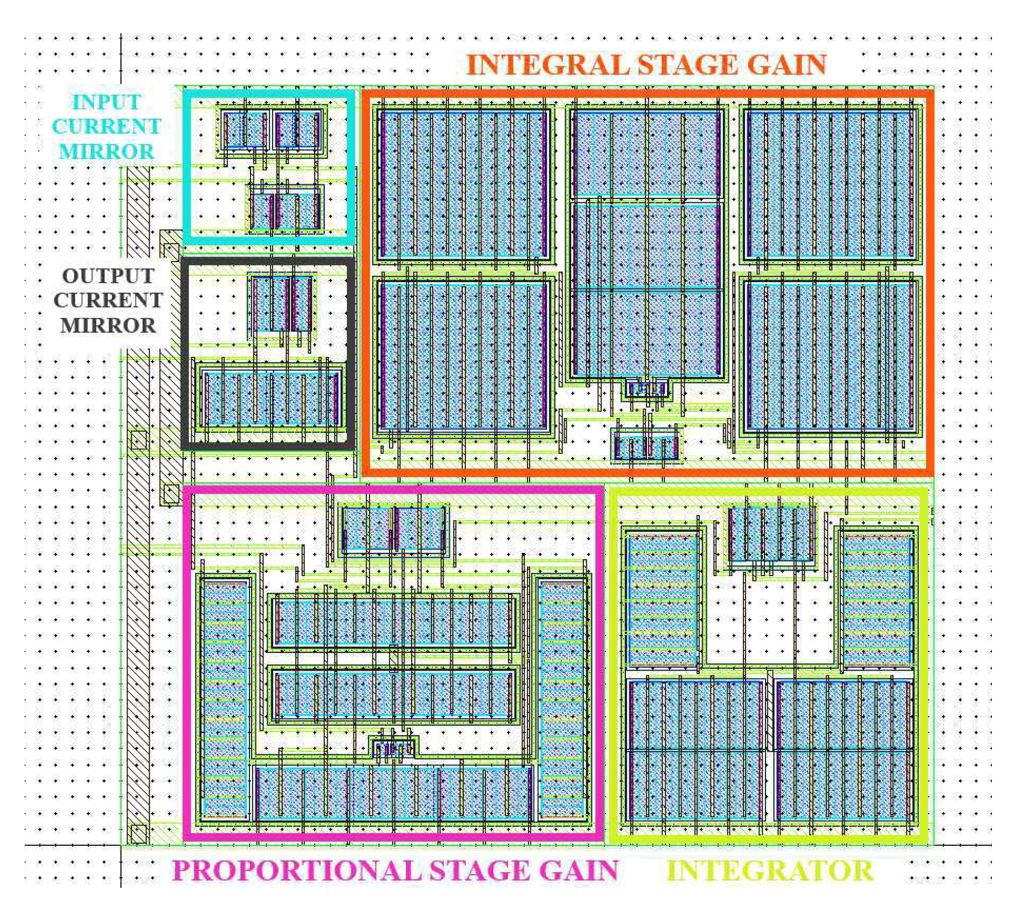
The layout design of the active core of the controller is demonstrated in
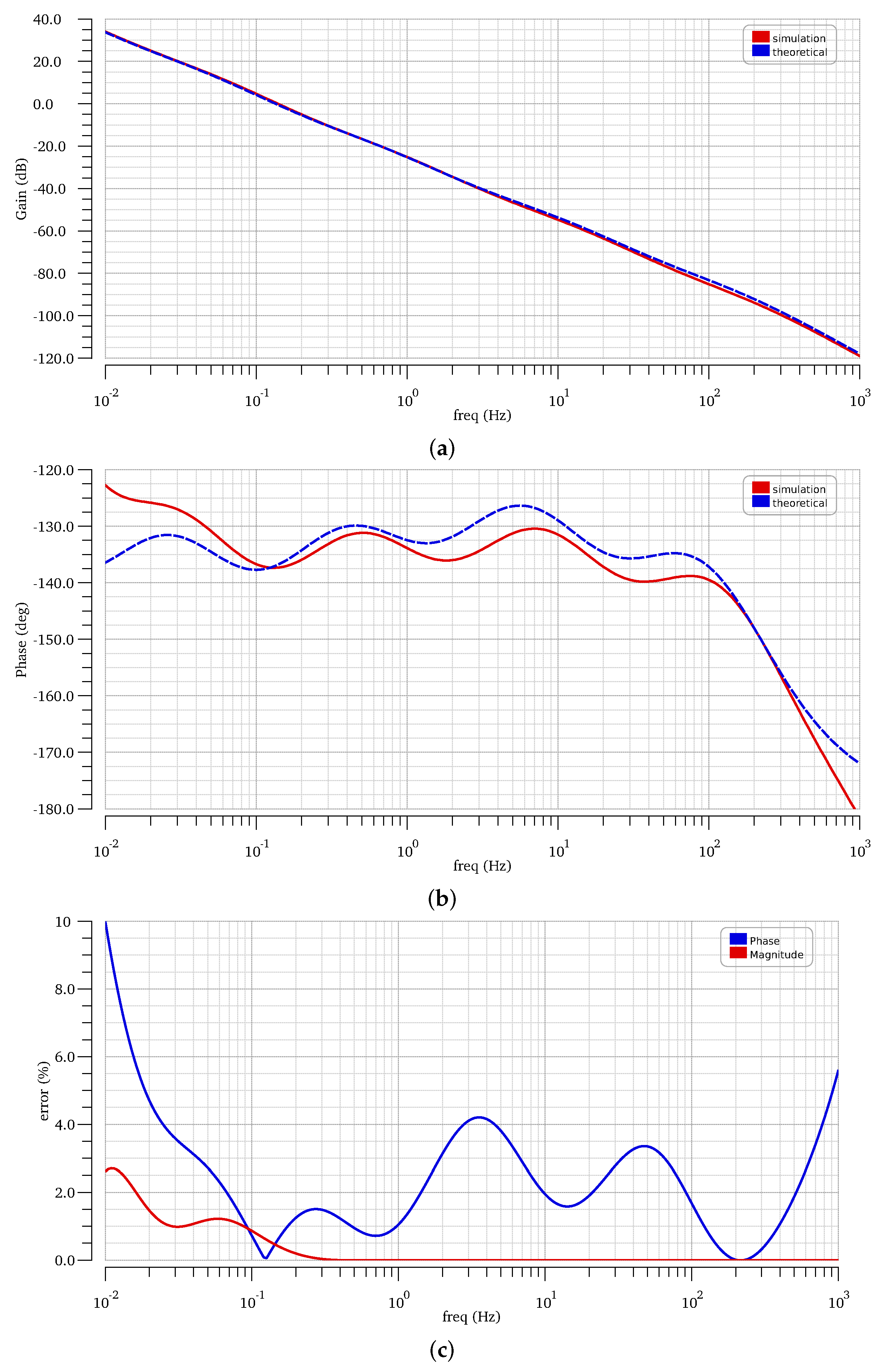
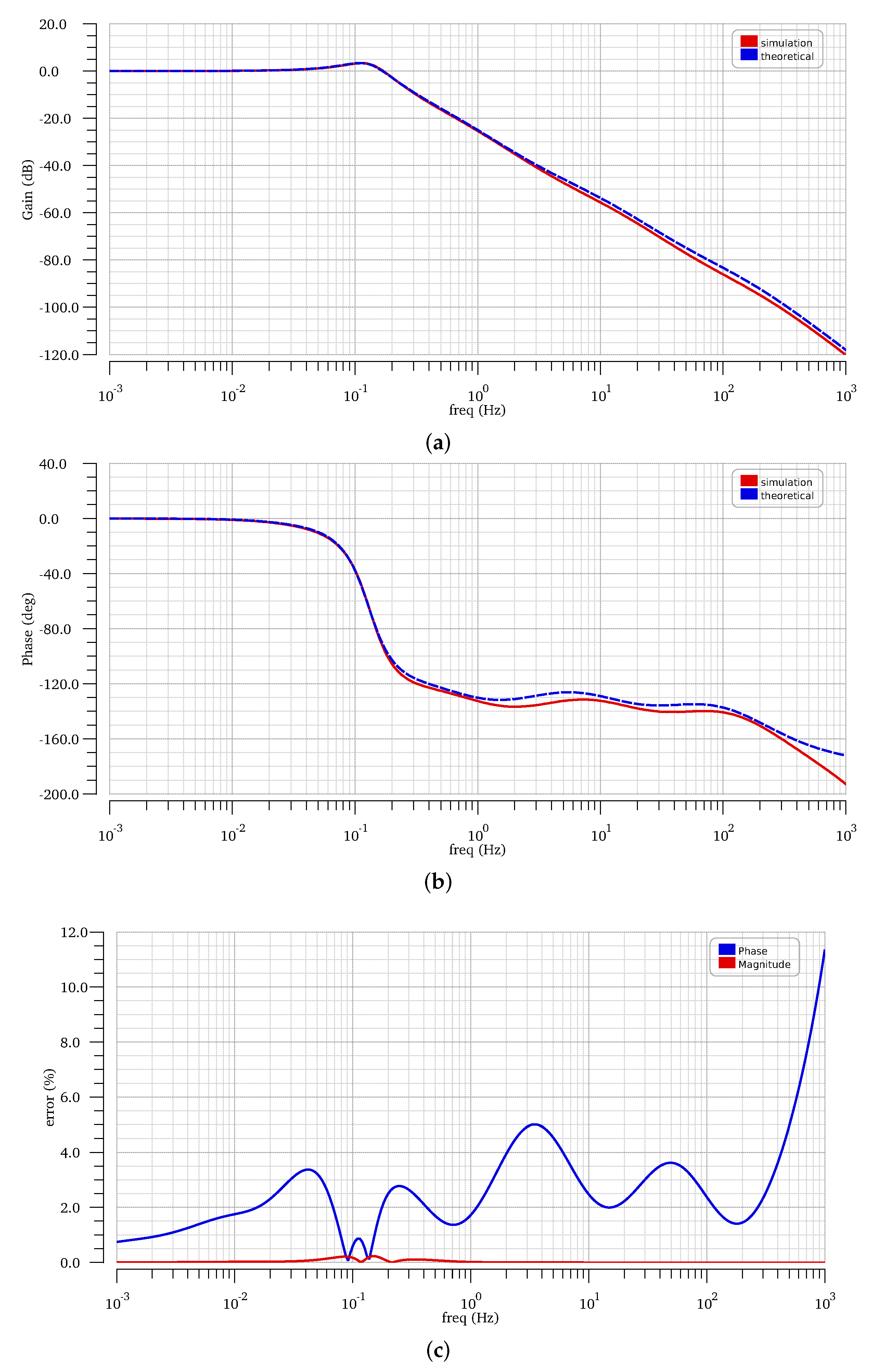
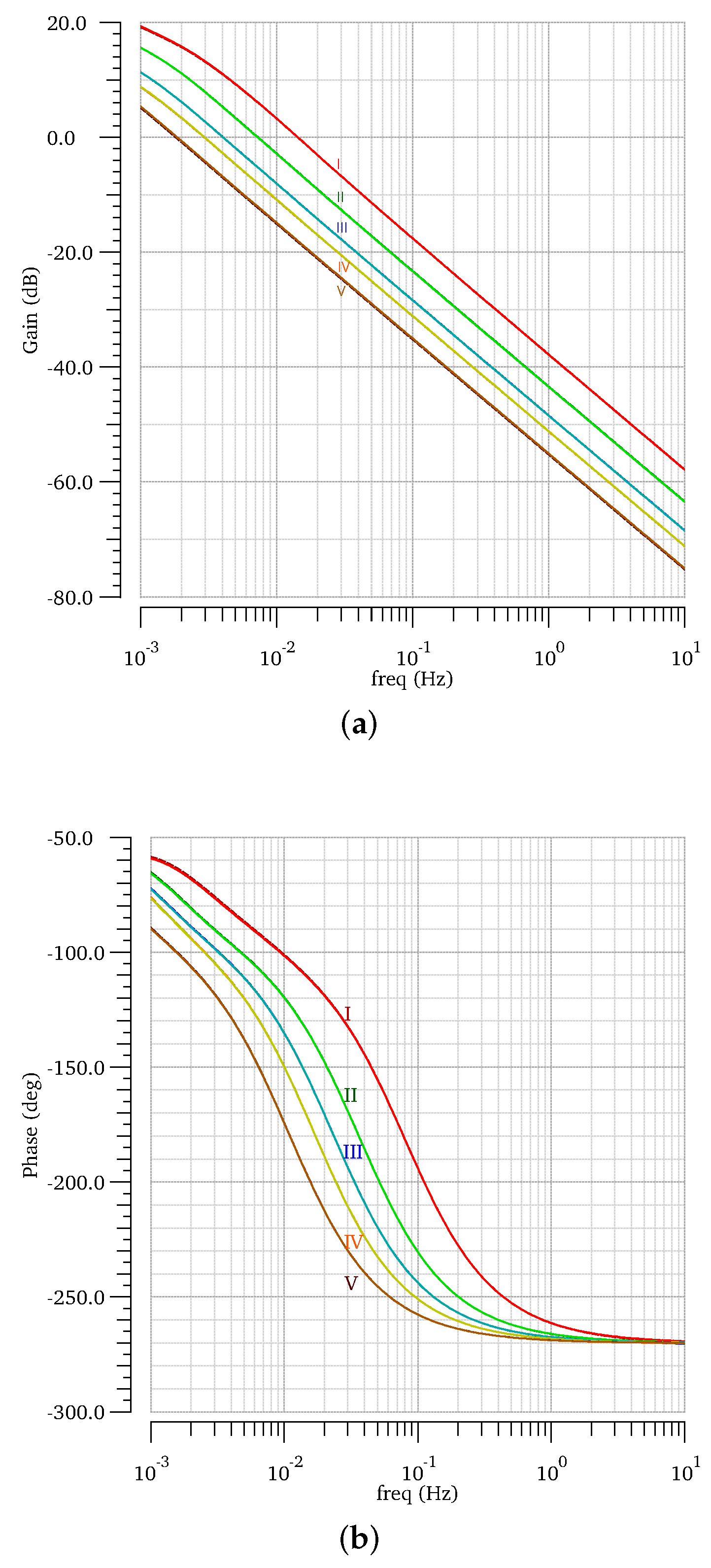
Figure 17. The obtained open-loop gain and phase responses of the controller-plant system are demonstrated in
Figure 18, for all the operating points presented in
Table 2. The phase margin for the operating points was measured as
,
,
,
, and
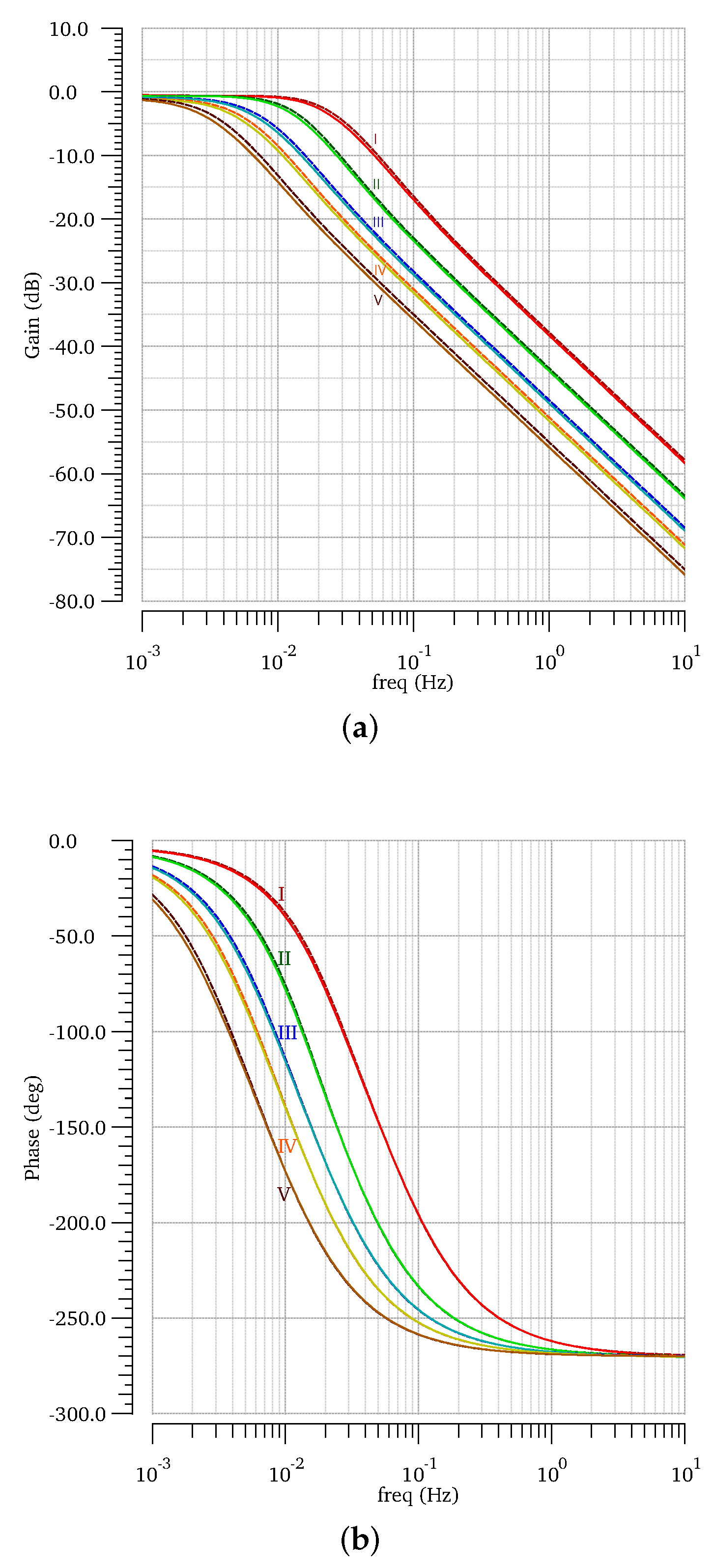
, respectively. From the derived results it is concluded that the phase margin increases as the height increases. The corresponding closed-loop responses are provided in
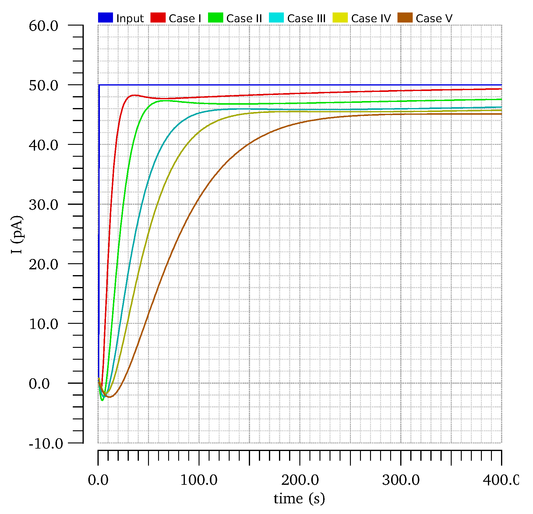
Figure 19, while the step responses for all the operating points are depicted in
Figure 20.
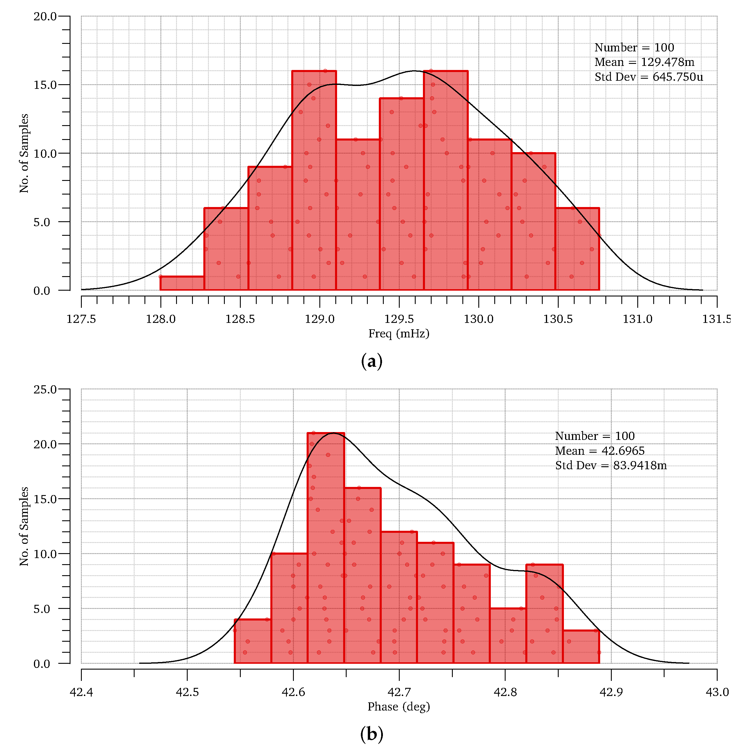
4. Conclusions
The proposed fractional-order DC motor I
D
controller offers an almost 50% reduction of the active component count as well as of power dissipation compared to that introduced in [
17]. With regards to the specifications, a 129.5 mHz gain-crossover frequency and 42.68
phase margin are achieved, with the corresponding nominal values being 158 mHz and 45
, respectively.
Moreover, a fully re-configurable controller topology suitable for controlling the level of liquid into two interacting tanks has also been presented in this work. The adjustment of the controller’s behavior into various conditions has been achieved through an appropriate adjustment of the corresponding DC bias currents, without altering the topology of the controller. The chip operates within V power supplies making the design very attractive from the reduced power dissipation point of view. In addition, the presented scheme is general and can be used in other applications, where a PI controller is required without changing its core, just by changing the values of the DC bias currents.
The simulation results presented in this article are very promising. Future research directions could be the following:
improvement of the consistency between theoretical and simulation results through the utilization of higher order approximation of fractional-order Laplacian operator,
fabrication and experimental verification of chips containing the proposed controller structures.

 ,
, 


