Exploring Efficient Acceleration Architecture for Winograd-Transformed Transposed Convolution of GANs on FPGAs ^†

Abstract

The acceleration architecture of transposed convolution layers is essential since transposed convolution operations, as critical components in the generative model of generative adversarial networks, are computationally intensive inherently. In addition, the pre-processing of inserting and padding with zeros for input feature maps causes many ineffective operations. Most of the already known FPGA (Field Programmable Gate Array) based architectures for convolution layers cannot tackle these issues. In this paper, we firstly propose a novel dataflow exploration through splitting the filters and its corresponding input feature maps into four sets and then applying the Winograd algorithm for fast processing with a high efficiency. Secondly, we present an underlying FPGA-based accelerator architecture that features owning processing units, with embedded parallel, pipelined, and buffered processing flow. At last, a parallelism-aware memory partition technique and the hardware-based design space are explored coordinating, respectively, for the required parallel operations and optimal design parameters. Experiments of several state-of-the-art GANs by our methods achieve an average performance of 639.2 GOPS on Xilinx ZCU102 and 162.5 GOPS on Xilinx VC706. In reference to a conventional optimized accelerator baseline, this work demonstrates an 8.6× (up to 11.7×) increase in processing performance, compared to below 2.2× improvement by the prior studies in the literature.

1. Introduction

With the wide application of deep neural networks [1], several convolution operation-based generative adversarial networks (GANs) [2,3,4] have emerged to accomplish computer vision-related tasks such as image generation/synthesis [5,6,7,8] and 3D object modeling [9,10]. We have also observed that transposed convolution, a specific-domain convolution kernel, is the primary operation involved in the generator component of GANs, while convolution is involved in another component of GANs called discriminator. Abundant prior acceleration works for convolution operation in several CNN models were presented based on field programmable gate arrays (FPGAs) [11,12,13,14,15,16]. More recently, increasing the performance of transposed convolution has been considered in a few works [17,18,19,20,21]. Transposed convolutions are always implemented by the way of the conventional convolution form directly. Unfortunately, such an equivalent convolution-based dataflow causes more than 70% ineffective operations. GNA [17] and Zhang’s work [18] solved the issue by designing a distinct computing strategy, so-called “Input-Oriented Mapping (IOM) method”, to eliminate expanding the sparsity of matrix at the origin. Referring to Eyerss [22] who focused on the common convolution, the authors of [19,20,21] concerned removing all the invalid operations in the sparse matrix multiplication.

By a different method from the works mentioned above, the fast Winograd algorithm is explored in this work for efficiently deploying the transposed convolution layers of GANs on FPGAs. The fast Winograd algorithm provides an efficient means of transforming 2D convolution operation into element-wise multiplication manipulation (EWMM) operation to reduce the computational complexity. In Winograd domain, multiplications of the elements in a constant transformation matrix are transformed to addition and shift operations, while implementing the addition and shift operations by logic units such as look-up-tables (LUTs) and flip-flops (FFs) on the FPGA should incur a lower computational cost. Several reported implementations [23,24] have demonstrated higher performance through deploying the Winograd-transformed common convolutional layers on FPGAs. To the best of our knowledge, this is the work to target extending the fast Winograd algorithm to the implementation of the transposed convolution layers of GANs on FPGAs.

This paper makes the following contributions:

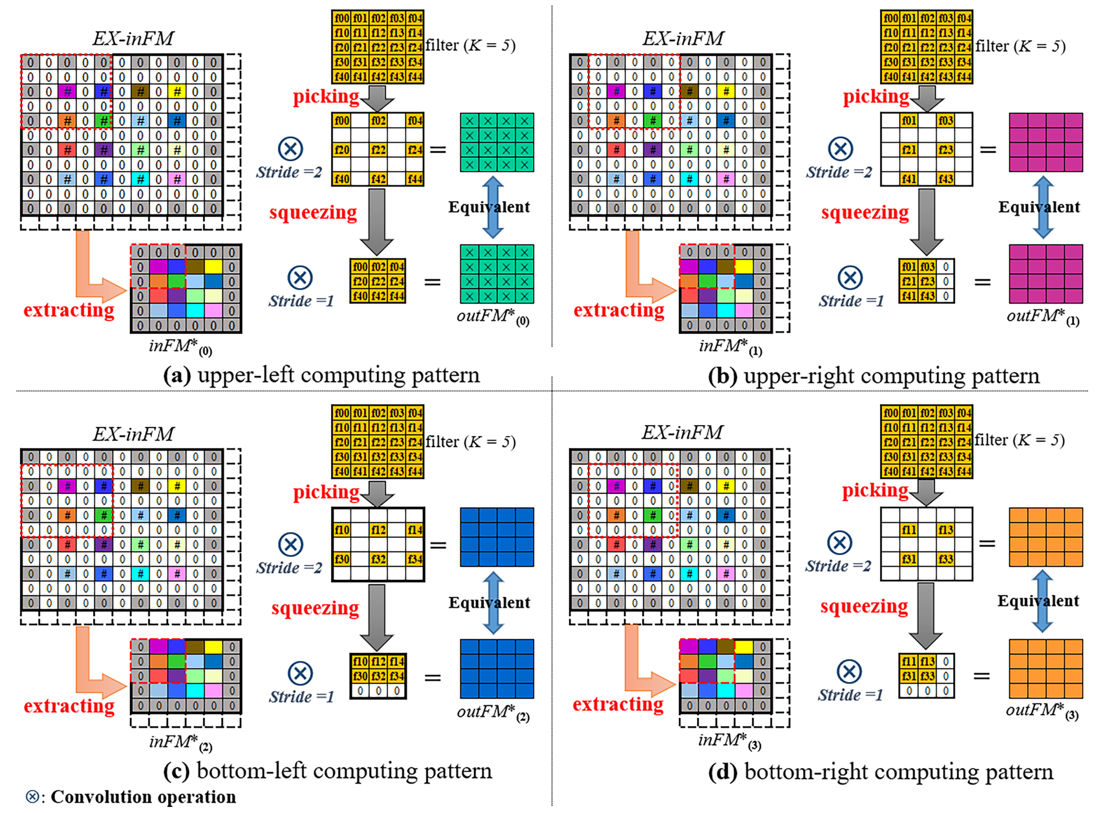
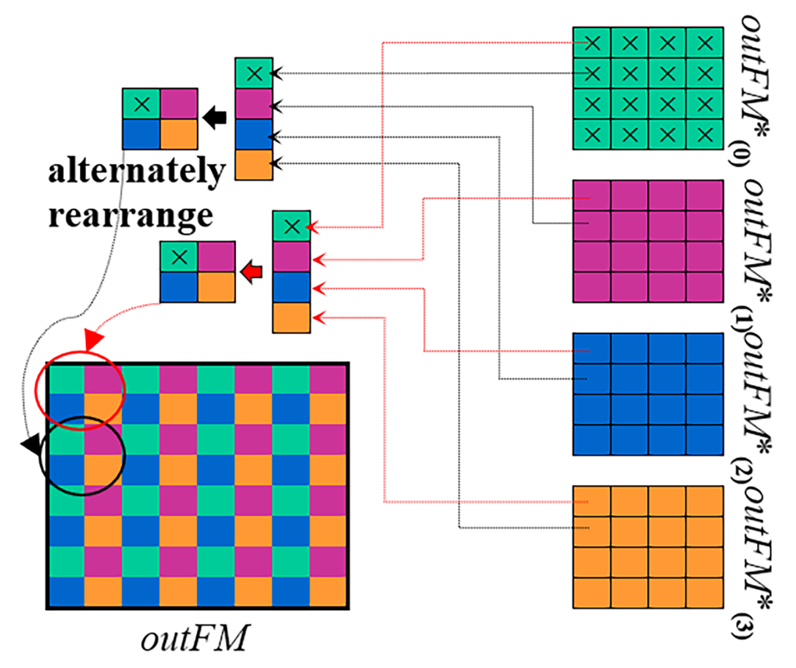
• We present a novel dataflow exploration, so-called Wino-transCONV, which eliminates all the computations involving 0 values and then implements the transposed convolution operation through adding the DECOMPOSITION and REARRANGEMENT stages in a regular Winograd-transformed convolution dataflow. This dataflow optimization allows a significant reduction in computational complexity.
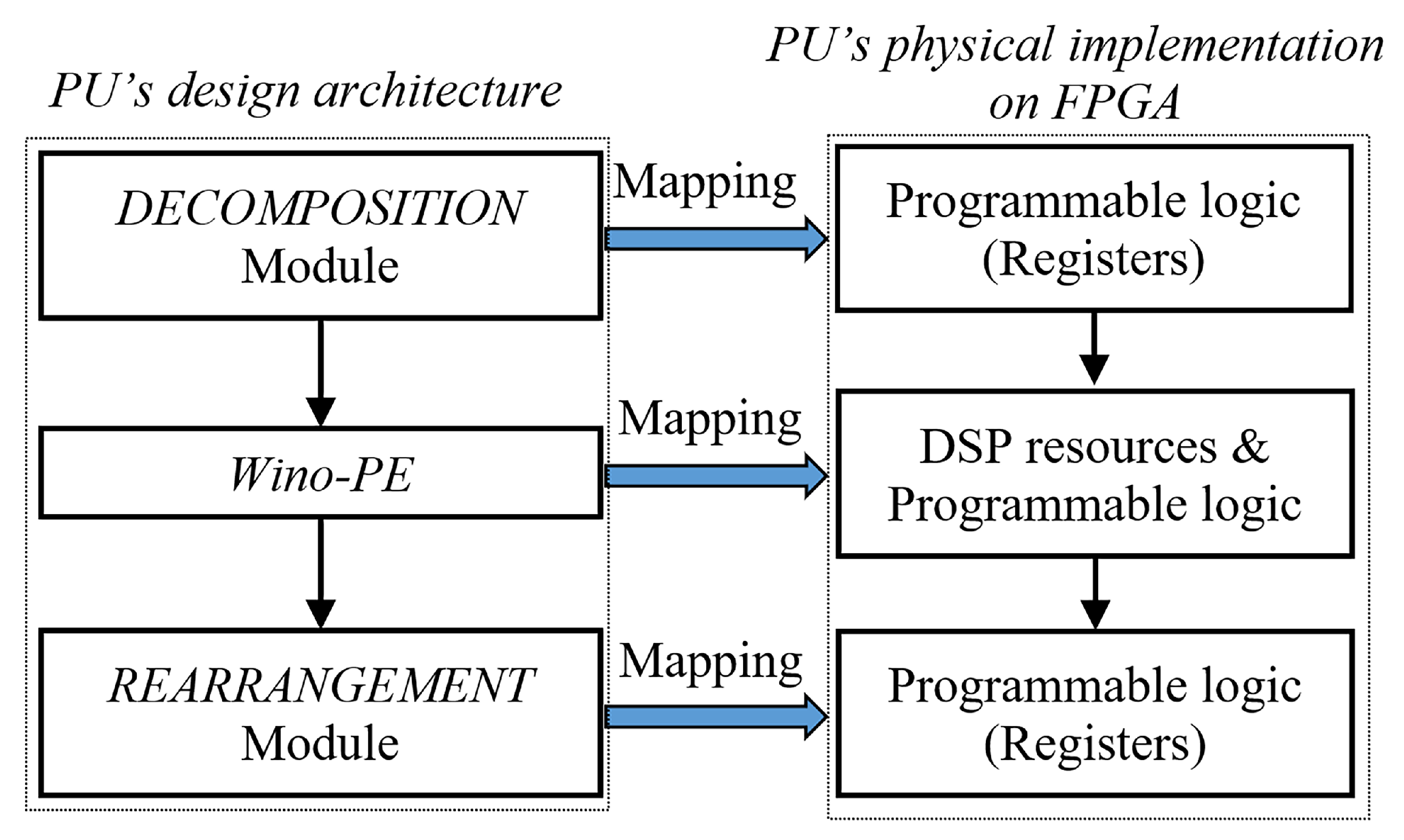
• We propose a custom architecture for implementing transposed convolution layers efficiently by mapping the multiple-stage Wino-transCONV dataflow to FPGA device with pre- and post-processing in place. The design structures include the processing unit and Buffer operating in a combined pipelined and parallel fashion.
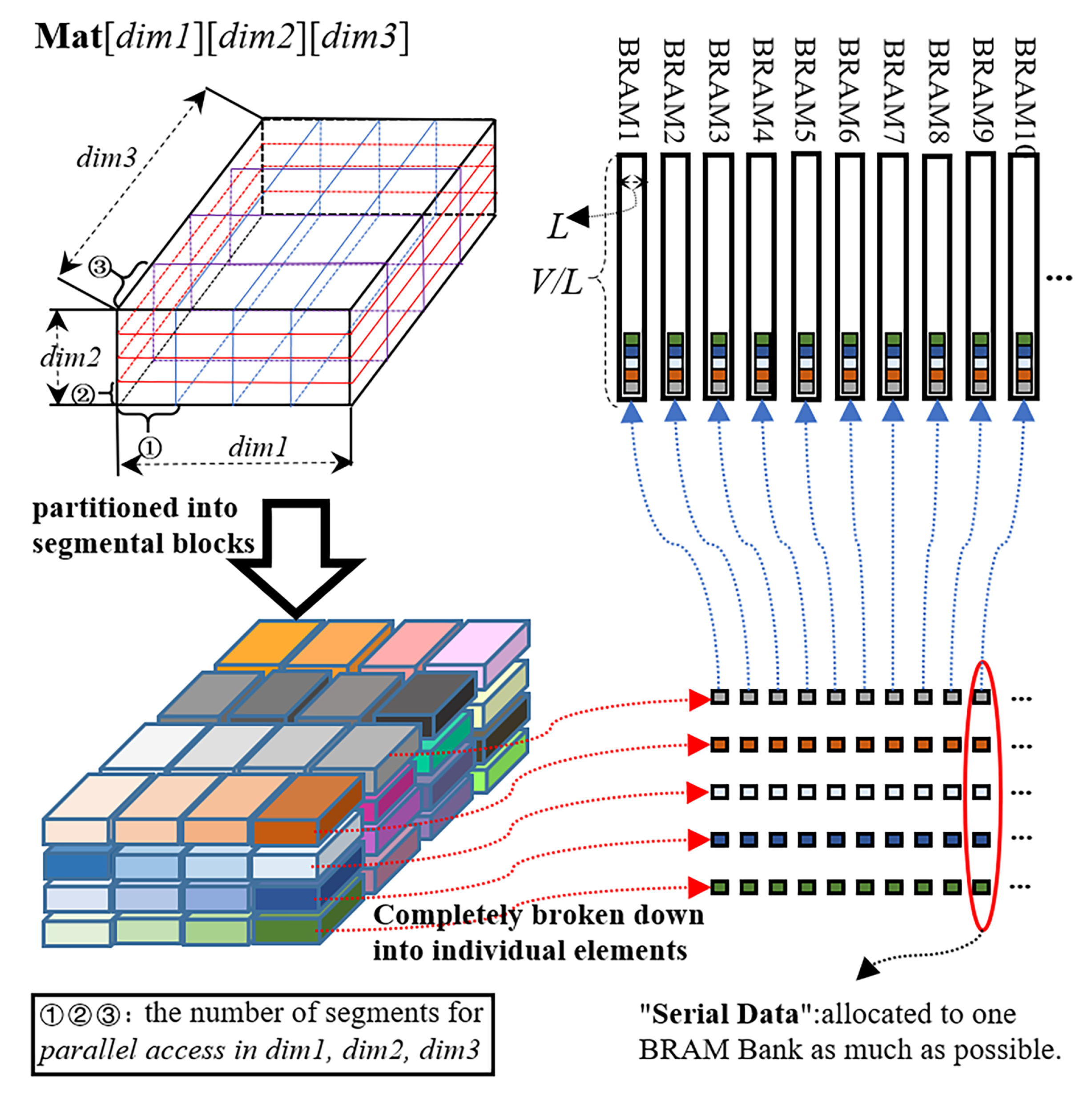
• We devise the memory parallelism-aware partition to achieve efficient data access in the paper. Meanwhile, the optimal hardware-based design space is also explored by analyzing the efficiency in resource allocations and the performance in computational executions.
• Several state-of-the-art GANs are verified on Xilinx FPGA devices by employing the proposed approaches in this paper.

The rest of this paper is organized as follows. Section 2 provides a brief description of some concepts regarding the fast Winograd algorithm and transposed convolution.The dataflow exploration is also highlighted in this section. Section 3 presents the custom architecture design optimized and implemented on FPGAs. Section 4 discusses the experimental verification results. Section 5 concludes this paper.

2. Dataflow Exploration

2.1. Transposed Convolution Dataflow Basics

The generator component of GANs features taking noise as input and generating samples, which involves a vast amount of transposed convolution operations. Figure 1 illustrates a representative data processing flow with regard to the Generative model of a GAN used for large-scale scene understanding challenge (LSUN) scene modeling [4]. Four layers of transposed convolutions (alias for fractionally-strided convolutions) are connected in series to convert the random noise representations into a high-resolution image. This paper is interested in exploring how to resource-efficiently boost the processing capabilities of implementing transposed convolution layers on FPGAs.

Similar to a general convolutional layer, a transposed convolution layer carries out the feature generation by applying N groups of the filters (each of the groups owning C×K×K filters) to C channels of the two-dimensional input feature maps (inFM, C×W×H) and then outputting N channels of the two-dimensional output feature maps (outFM, N×2W×2H), as shown in Figure 2. As detailed in Figure 3, transposed convolution can be mapped into the conventional convolution dataflow, after the inFM is inserted and padded with zeros where appropriate to obtain the expanded input feature map (EX-inFM).

2.2. Winograd Transformation Basics

As shown in the equation below, the 2D convolution can be transformed in the fast Winograd algorithm [25].

$$\mathbf{OUT}={\mathbf{A}}^T·\left[(\mathbf{G}·\mathit{F}·{\mathbf{G}}^T)\odot ({\mathbf{B}}^T·\mathit{IN}·\mathbf{B})\right]·\mathbf{A}$$

(1)

Suppose that: IN has a size of n×n (n = m + r - 1); OUT has a size of m×m; F has a size of r×r; and “⊙” symbolizes an Element-Wise Matrix Multiplication (EWMM).

Both transformation matrices, G and B, are applied to, respectively, convert the weight filter ($\mathbf{F}$) and the input feature map ($\mathbf{IN}$) to the Winograd domain first. Then, in the Winograd domain, the two results are multiplied befor their outcome is further converted back by the third transformation matrix, A, to obtain the output feature map OUT. In one example case, in which m = 2 and r = 3, the Winograd transformation matrices ${\mathbf{A}}^T$, ${\mathbf{B}}^T$, and G are defined as follows:

$${\mathbf{B}}^T=\left[\begin{array}{cccc}1& 0& -1& 0\\ 0& 1& 1& 0\\ 0& -1& 1& 0\\ 0& 1& 0& -1\end{array}\right],\mathbf{G}=\left[\begin{array}{ccc}1& 0& 0\\ \frac{1}{2}& \frac{1}{2}& \frac{1}{2}\\ \frac{1}{2}& -\frac{1}{2}& \frac{1}{2}\\ 0& 0& 1\end{array}\right],{\mathbf{A}}^T=\left[\begin{array}{cccc}1& 1& 1& 0\\ 0& 1& -1& -1\end{array}\right]$$

(2)

2.3. Wino-transCONV Dataflow Exploration

As discussed above, our purpose is to remove void operations and reduce computational complexity. Foremost, we present DECOMPOSITION processing to eliminate void operations. As exhibited in Figure 4, there exist four (2×2) computing patterns for a 5×5 sized filter sliding up, down, left, and right over a 6×6 sized tile-window of the EX-inFM for operations. Specifically, the upper-left computing pattern in Figure 5 correspondingly generates the green-colored grids (also denoted with “×”) for the outFM, as depicted in Figure 5a and  Figure 6. For the three other computing patterns, the same principle is applied to generate pink, blue and orange colored grids as, respectively, shown in Figure 5b–d. Those 25 grids ($f_{0\sim 4,0\sim 4}$) belonging to the filter window are divided into and distributed across the four sub-filters with the irregular numbers of non-zero values (9+6+6+4). Figure 5 illustrates the detailed evolution dissolving a transposed convolution into four equivalent convolutions during the DECOMPOSITION process. More clearly, we pick the non-zero values of the filter and then squeeze the sparse matrix to the dense matrix. This way, one transposed convolution processing task over the 5×5 sized filters can be distributed into the four common convolution subroutines operated with smaller 3×3 sized filters.

Subsequently, the standard Winograd algorithm is possibly applied to implement the four general convolutions subroutines to reduce computational cost. It is noted that Figure 5 demonstrates the effectiveness of the offered data compression pre-processing for exploring the application of fast Winograd algorithm, when the filter is taken on the route of picking and squeezing for the minimum operations with inFM*. This matches the fact that, for an effective transformation, those conventional convolutions with the core size not exceeding 3×3 [23,24] are required by the execution of the fast Winograd algorithm.

Eventually, the four intermediate outputs in Figure 6 are alternately rearranged into the final outFM as necessary for the post-processing shown in Figure 5.

An overview of the provided Wino-transCONV dataflow is exhibited in Figure 7. With the exception of the standard fast Winograd algorithm ($S2$–$S4$), the two new stages, namely DECOMPOSITION (S1) and REARRANGEMENT (S5), are involved in this paper. A detailed explanation for DECOMPOSITION is given above (cf. Figure 4 and  Figure 5). Particularly during the processing of S1, the complete filter window with a size of K×K, which slides over the (n+1)×(n+1) sized tile-window of inFM, is split into four effective sub-filter windows. Next, each of those four effective sub-filter windows is operated on its corresponding sub-inFM window pattern. The processing of S5 is relatively simple, as four m × m sized intermediate output patterns are produced after S4 and alternately rearranged into one 2 m×2 m sized outFM. According to the standard fast Winograd algorithm, S2 implements matrix transformations for both the input feature map and the filter, while S3 implements EWMMs and S4 implements matrix transformations for the output feature map.

The computational complexity of Wino-transCONV dataflow can be measured via the amount of the multiplication operands required to occupy the DSP resources on an FPGA device. For quantitative estimation, the following equations are derived:

$$Mul{t}_{Direct-CONV}=\left(2H-1\right)\times \left(2W-1\right)\times K\times K$$

(3)

and

$$Mul{t}_{Direct-CONV-eff}=H\times W\times K\times K$$

(4)

Here, $Mul{t}_{Direct-CONV}$ represents the number of multipliers needed for the convolution descendent from a direct transformation of the transposed convolution [4] when a K×K sized filter is applied on a W×H sized inFM. $Mul{t}_{Direct-CONV-eff}$ corresponds to the number of multipliers needed after a further removal of all the invalid operations [17,18,19,20,21].

For our Wino-transCONV dataflow, the number of multipliers required may be determined as follows simultaneously.

$$Mul{t}_{Wino-transCONV}=4·⌊\frac{H-(n-m)+2}{m}⌋·⌊\frac{W-(n-m)+2}{m}⌋·n^2$$

(5)

Table 1. Computational resource usage analysis.

inFM	Filter	Methods	Mum_of Operations			Normalized
(W×H)	(K×K)		mult (*)	add (+)	total_equiv_add ${}^1$
8×8	5×5	Direct-CONV [4]	5625	5400	95,400	1
		Direct-CONV-eff [17,18,19,20,21]	1600	1536	27,136	0.284
		Wino-transCONV(m = 4)	576	10,048	19,264	0.201
		Wino-transCONV(m = 2)	1024	4928	21,312	0.223
	4×4	Direct-CONV [4]	3600	3375	60,975	1
		Direct-CONV-eff [17,18,19,20,21]	1024	960	19,394	0.318
		Wino-transCONV(m = 4)	576	10,048	19,264	0.315
		Wino-transCONV(m = 2)	1024	4928	21,312	0.349
16×16	5×5	Direct-CONV [4]	24,025	23,064	407,464	1
		Direct-CONV-eff [17,18,19,20,21]	6400	6144	108544	0.266
		Wino-transCONV(m = 4)	2304	40,192	77,056	0.189
		Wino-transCONV(m = 2)	4096	19,712	85,248	0.209
	4×4	Direct-CONV [4]	15,376	14,415	260,431	1
		Direct-CONV-eff [17,18,19,20,21]	4096	3840	77564	0.297
		Wino-transCONV(m = 4)	2304	40,192	77,056	0.295
		Wino-transCONV(m = 2)	4096	19,712	85,248	0.327
64×64	5×5	Direct-CONV [4]	403,225	387,096	6,838,696	1
		Direct-CONV-eff [17,18,19,20,21]	102,400	98,304	1,736,704	0.253
		Wino-transCONV(m = 4)	36,864	643,072	1,232,896	0.18
		Wino-transCONV(m = 2)	65,536	315,392	1,363,968	0.199
	4×4	Direct-CONV [4]	258064	241,935	4,370,959	1
		Direct-CONV-eff [17,18,19,20,21]	65,536	61440	1,241,084	0.283
		Wino-transCONV(m = 4)	36,864	643,072	1,232,896	0.282
		Wino-transCONV(m = 2)	65,536	315,392	1,363,968	0.312
128×128	5×5	Direct-CONV [4]	1,625,625	1,560,600	27570600	1
		Direct-CONV-eff [17,18,19,20,21]	409,600	393,216	6,946,816	0.251
		Wino-transCONV(m = 4)	147,456	2,572,288	4,931,584	0.178
		Wino-transCONV(m = 2)	262,144	1,261,568	5,455,872	0.197
	4×4	Direct-CONV [4]	1040400	975,375	17,621,775	1
		Direct-CONV-eff [17,18,19,20,21]	262,144	245,760	4,964,352	0.281
		Wino-transCONV(m = 4)	147,456	2,572,288	4,931,584	0.279
		Wino-transCONV(m = 2)	262,144	1,261,568	5,455,872	0.309

${}^1$ total_equiv_add = mult * L + add, where L = 16.

lists some comparison analysis results for the computing resource usage deemed among different acceleration platforms. In the table, the terms mult, add, and total_equiv_add denote the respective numbers of multiplications, additions, and  total equivalent additions thus calculated. Without loss of generality, an L bit-width (fixed point) multiplication can be equivalently dissolved into L times the same bit-width additions. In this analysis, L = 16 is assumed. In Table 1, the Wino-transCONV dataflow results in the minimized multiplications through being replaced with reasonably increased additions. Thus, we advantageously trade the DSP resources with the LUT-plus-FF resources, which should be abundantly available nowadays on FPGAs. In this way, it should deliver a higher degree of implementation parallelism than the prior studies. In terms of the normalized factor, the Wino-transCONV approach reduces the number of operations approximately by 70–80%, compared to the Direct-CONV. It also requires fewer resources than Direct-CONV-eff by almost one third. Further referring to Table 1, a close examination suggests that the transforming properties associated with the Wino-transCONV should not be influenced by the size of inFM, although they exert the reduction effect more prominently with 5 × 5 filters than 4 × 4 ones.

3. Design and Implementation

3.1. Architecture-Wise Optimization

Figure 8 illustrates the overall custom architecture design for the proposed dataflow exploration. In the figure, numerous datasets are involved, including inFMs, filters, and outFMs, all in batches to transport between on- and off-chip via, e.g., the AXI-Stream interface connection provided by the FPGA device. To overlap the computation time and data transfer time, the double line buffer [23] is adopted to realize ping-pang data exchange operations in this paper. A processing unit (PU) is specifically designed to accommodate the execution procedure, as specified in Figure 8 for a common transposed convolution operation. Then, Multiple PUs will be formed in an array to complete the entire Wino-transCONV dataflow in parallel. A tile-window of the inFM would be taken from the line buffer and then subsequently sent to a relevant PU along with a filter, while the PU generates the result to an outFM. As  detailed in Figure 8, each of those PUs consists of a DECOMPOSITION pre-processing module, a Winograd Processing Element (Wino-PE) module, and a REARRANGEMENT post-processing module, all being mapped into DSPs or LUT-register resources on FPGA, as exhibited in Figure 9.

To raise the processing capabilities at the architecture level, this paper investigates some possible implementation strategies for optimally balancing various design conditions such as hardware parallelism vs. network performance. We have observed that the transposed convolution in the algorithm can tap into two kinds of concurrent executions, namely the parallel processing among FMs and inside an FM [26]. Moreover, pipeline is regarded as an indispensable means that could possibly be taken to lift up the performance of an accelerator system. The strategies of inter-PU parallelism, intra-PU parallelism, and intra-PU pipeline are used for balancing the various conditions such as parallelism, peak performance, and resource consumption as follows:

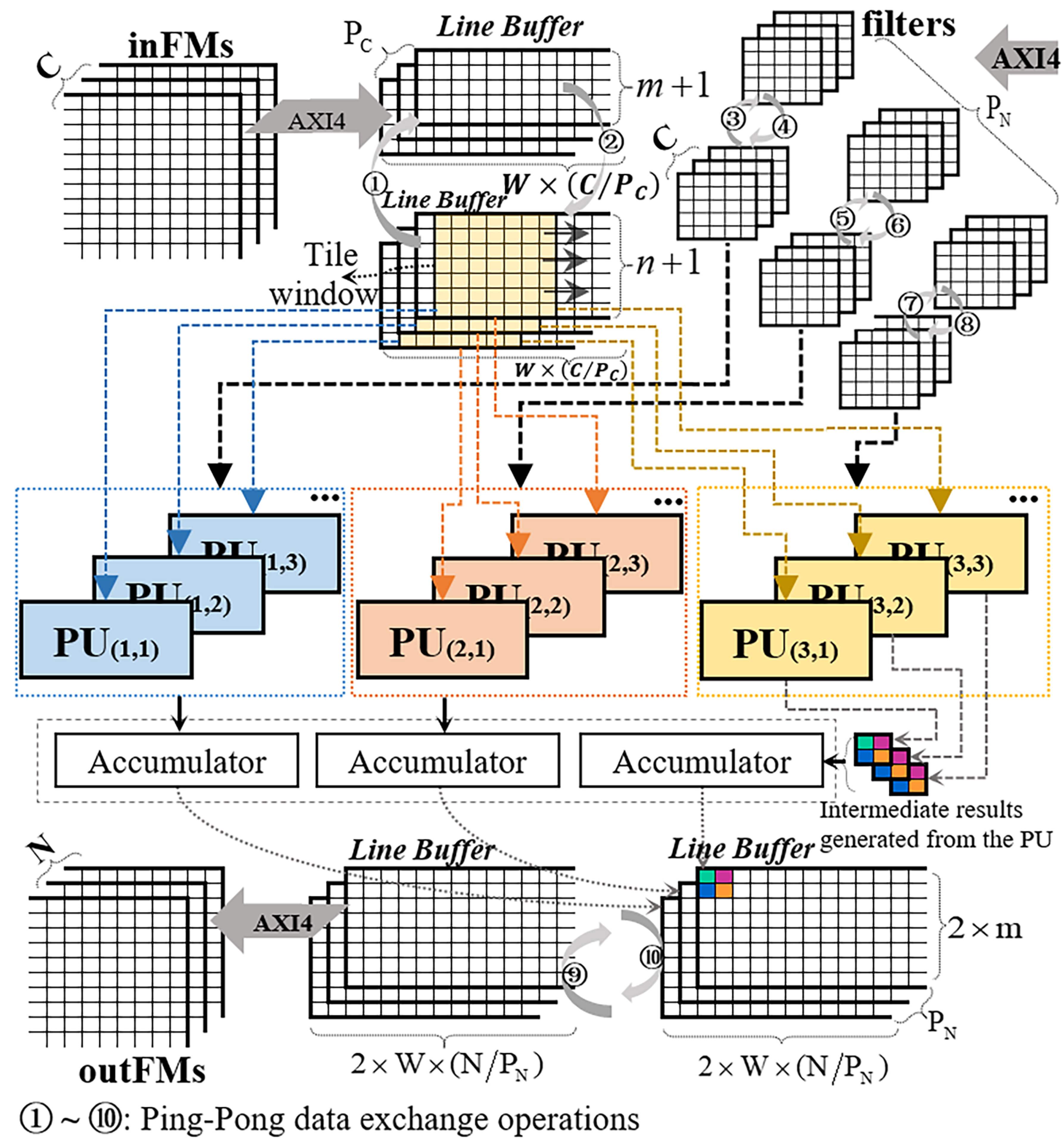
• Inter-PU parallelism: In the design, each PU is accountable for processing the data from one of the C channels of inFMs to one of the N channels of outFMs. Suppose that $P_C$ and $P_N$ denote parallel undertakings of inFMs and outFMs, respectively. Therefore, there are in total ($P_C$×$P_N$) PUs to execute their individual operations in parallel.
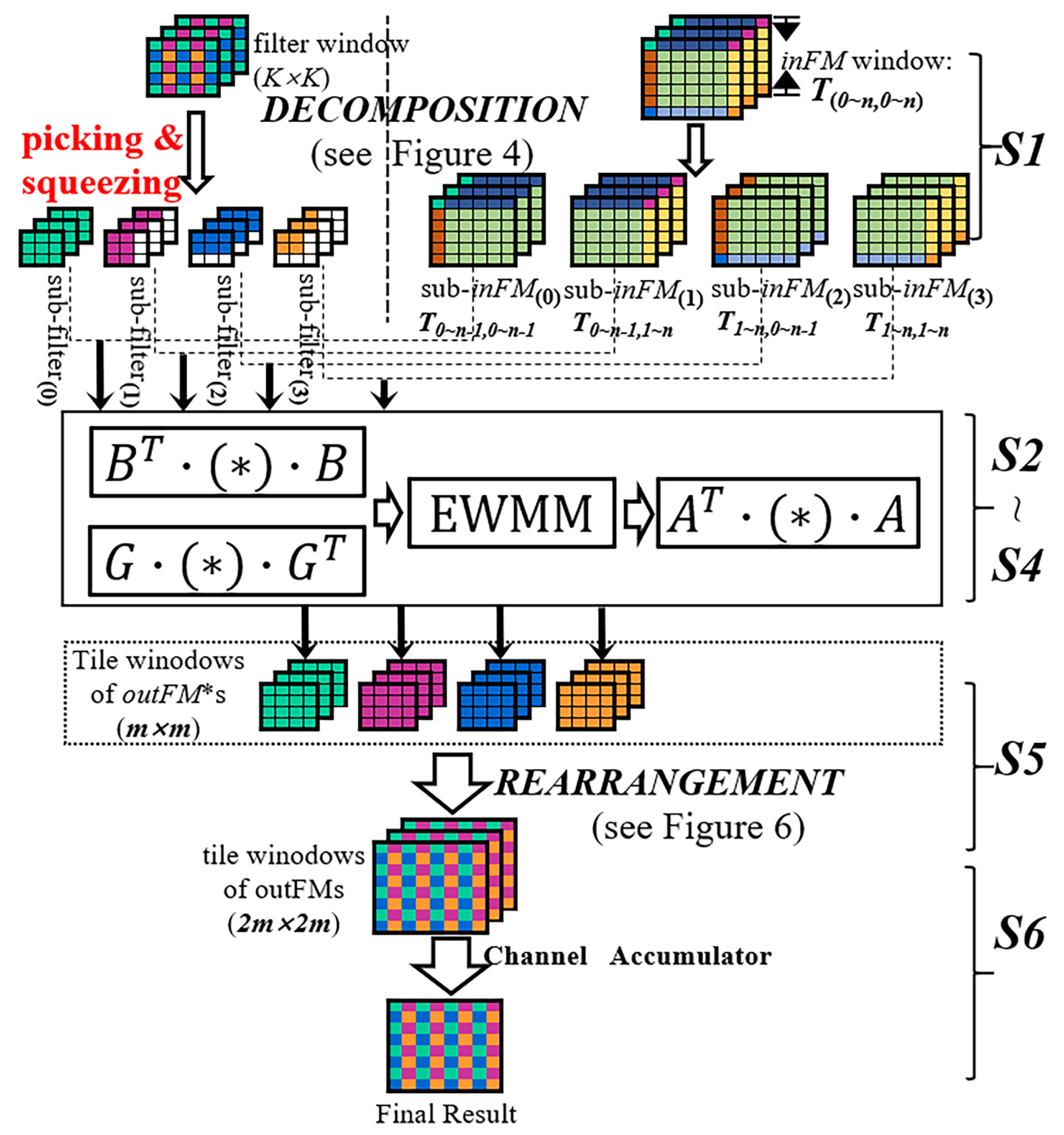
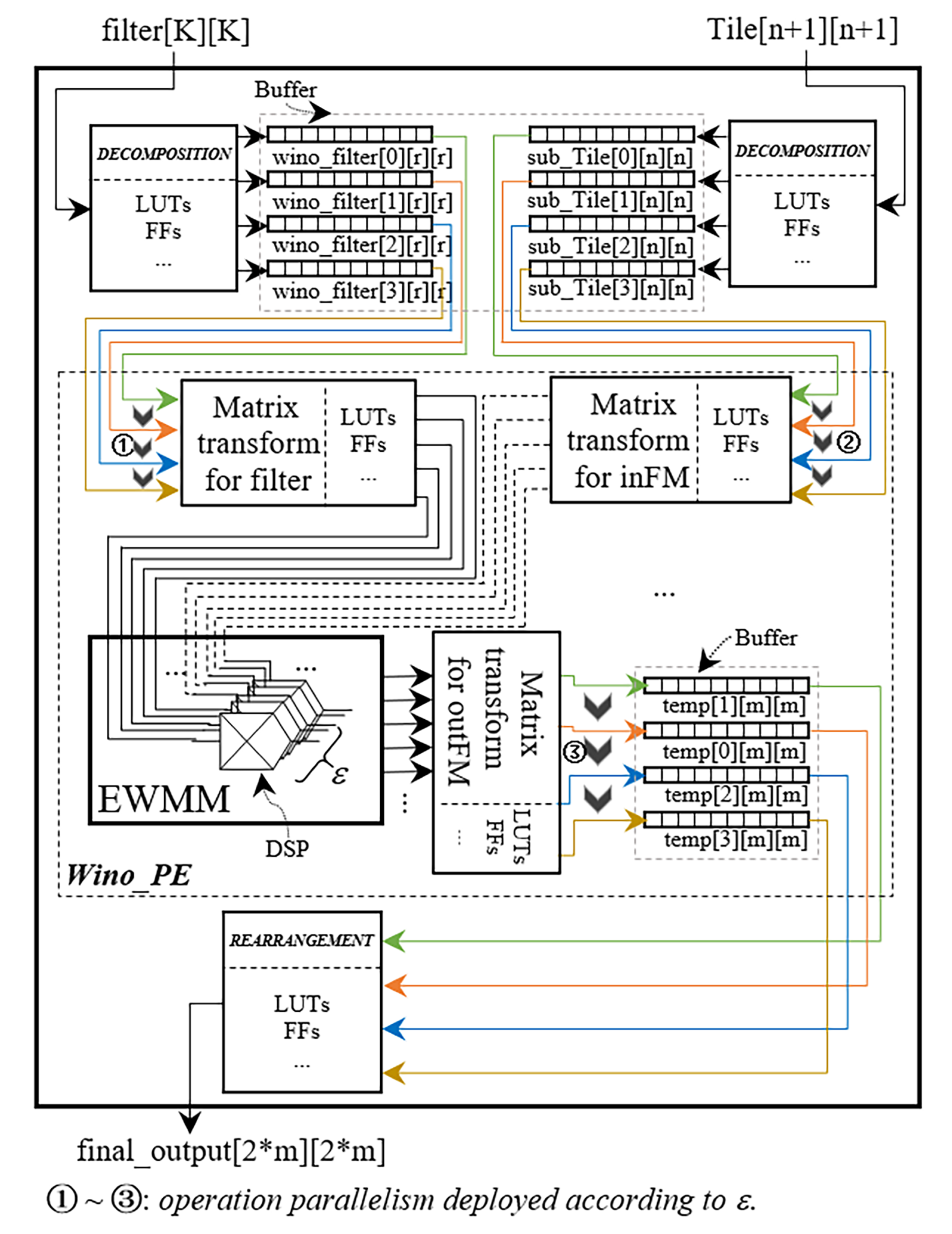
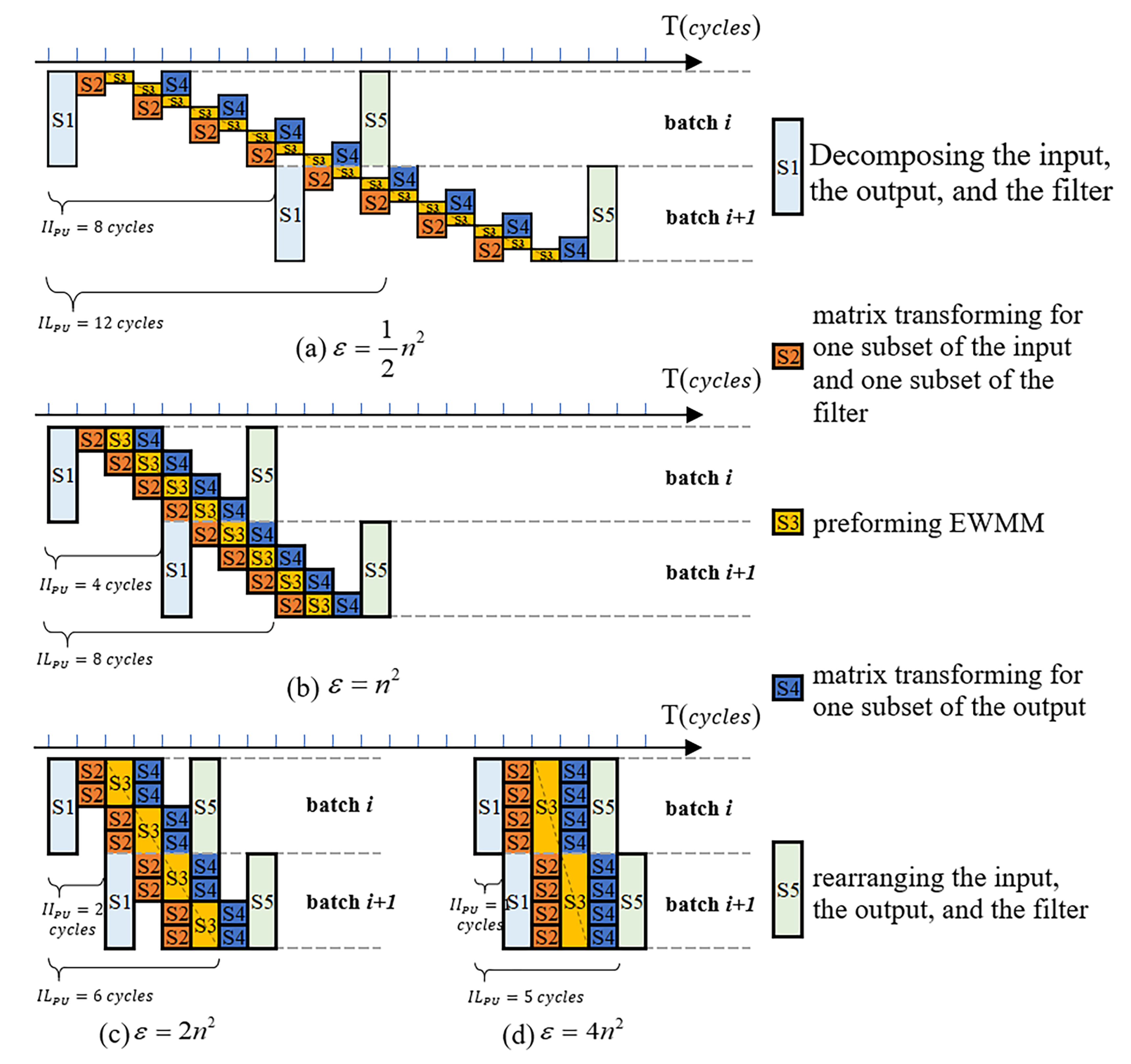
• Intra-PU parallelism: According to Figure 7, the function of Winograd processing inside a single PU is responsible for sequentially processing four pairs of the decomposed data, i.e., (sub-inFMs and sub-filters). Nevertheless, those four pairs can also be individually operated upon in parallel. Thus, the operational speed is improved, although at the expense of additional DSP blocks and programable logic resources being needed. It should be conceded that a single PU having consumed excessive DSP blocks would in practice result in the reduction to the degree of inter-PU parallelism, which must fall towards a smaller measure in terms of the number of ($P_C$×$P_N$). This is because the total number of DSP resources available on an FPGA device is always capped.
• Intra-PU Pipeline: In a PU structure, Steps S–S4 can be effectively pipelined according to the dataflow of Wino-transCONV given in Figure 7 except for S1 and S5. This is because the DECOMPOSITION (S1) and the REARRANGEMENT (S5) for those four pairs of data (sub-inFMs and sub-filters) cannot share one common set of hardware on a time division multiplexing basis.

3.2. Processing Unit Detail vs. Intra-PU Parallelism & Pipeline

Figure 10 describes a design structure for the PU. The programmable logic resources abundantly available in FPGA are utilized to execute all the matrix transformations (in the Wino-PE module), DECOMPOSITION processing, and REARRANGEMENT processing. The values of matrices (i.e., A, B, and G) in matrix transformations are computed offline and they normally take simple constants such as +1, −1, and $\raisebox{1ex}{$1$}\!\left/ \!\raisebox{-1ex}{$2$}\right.$, while both DECOMPOSITION and REARRANGEMENT only involve the operations regarding data formatting.

Element-wise matrix multiplication in the Wino-PE is the only module that is performed by the DSP blocks in the form of MAC units. Assuming it is denoted as the number of DSP (MAC) blocks required to achieve such EWMM in a PU, necessitating for execution in parallel and, further, one DSP block carries out fixed point multiplication in a bit-width of on FPGA device, to exercise the maximum parallelism, $\epsilon =4\times n\times n\times (\raisebox{1ex}{$\chi $}\!\left/ \!\raisebox{-1ex}{$\eta $}\right.$) DSP blocks would be required to operate, where $\chi$ symbolizes the original bit-width dictated by the algorithm itself. In this work $\chi$ and $\eta$ and are specifically chosen to be the same and equal to 16 bits (considering an elementary DSP unit as 18b × 25b multiplier embedded in FPGA).

It is preliminarily emphasized with regard to the intra-PU parallelism and pipeline in Section 3.1 that, on the one hand, there exist six possible configurations of concurrency for a typical instance where n = 6, i.e., $\epsilon$⊆{144, 72, 36, 18, 9, 3}. As exhibited in

Table 2. Concurrency vs. throughput for EWMM (in the case of the 6 × 6 sized tile-window).

$\left(\mathit{\epsilon }\right)$	144	72	36	18	9	3
Cycles required to complete EWMM	1	2	4	8	16	48

, the larger $\epsilon$ is, the fewer cycles are required to complete the operations, which indicates that the latency becomes shorter over a single PU. As a result, more EWMM operations would be conducted in concurrency, hitherto increasing the overall processing throughput.

On the other hand, the pipeline technique is applied in conjunction with a parallel strategy. The timing diagrams for a single PU with four typical values are given in Figure 11. They demonstrate a coherent parallel–pipeline scheme for executing all the necessary operations in PU. Actually, the actual value of $\epsilon$ should have impact on the initiation interval and the interval latency (II and IL [27,28]) as far as the pipeline design considered. ${\mathit{II}}_{PU}$ and ${\mathit{IL}}_{PU}$ can be estimated referring to the above analysis:

$$I{I}_{PU}=\frac{4n^2}{\epsilon }·I{I}_s,I{L}_{PU}=\left(\frac{4n^2}{\epsilon }-1\right)I{I}_s+I{L}_s$$

(6)

where ${\mathit{II}}_S$ and ${\mathit{IL}}_S$ are the values of II and IL$@\epsilon =4n^2$ supposing ${\mathit{II}}_S$ = 1 cycles while ${\mathit{IL}}_S$ = 5 cycles in Figure 11 for simplicity, which are denoted as the standard reference measure. ${\mathit{II}}_S$ and ${\mathit{IL}}_S$ are further utilized to explore the design space in Section 3.4.

The correlation regarding operational performance vs. $\epsilon$ is characterized on the Xilinx ZCU102 platform and evaluated with Xilinx Tool. As proposed in Figure 12, the processing performance in terms of Giga Operations Per Second (GOPS) goes up linearly with $\epsilon$, while the energy efficiency denoted as GOPS/W somehow increases logarithmically with $\epsilon$. This means that, although the processing performance does proportionally increase with the number of DSP blocks working in parallel, the pace to raise the energy efficiency by aligning more DSP blocks in concurrency may gradually slow down with $\epsilon$ growing larger. The reason may be attributed to the fact that a high degree of parallelism may cause lengthy and excessive interconnect wires on FPGA device and, in such conditions, the ratio of the DSP over the whole implementation with regard to power consumption would also gradually go up, typically from 1% (when $\epsilon$ = 3) to 40% (when $\epsilon$ = 144).

Based on inter-PU parallelism and intra-PU parallelism, the total number of DSP blocks required to realize all the ($P_C$×$P_N$) PUs in an FPGA may be predicted by:

$$num\_DSP=\epsilon \times P_C\times P_N$$

(7)

3.3. Memory Sharing—Access and Partition

To have memory availble to be accessed, a parallelism-aware partition technique is taken into consideration. The on-chip data of inFMs, filters, and outFMs can be described as respective multi-dimensional matrices (Mats).

In principle, the data in a relevant Mats are partitioned into a certain number of segments; thus, they can be accessed in parallel to coordinate the parallel operations required.

Table 3. Specifications of memory partition.

	(Number of segments for parallel access)×(size of the segment)				Total number of the		Data volume defined for one memory block in
	dim1	dim2	dim3	dim4	memory blocks required		type (= 16 bits)
inFM	(m+n+2)×(1)	(n+1)×[W/(n+1)]	(PC)×(C/ PC)	–	(m+n+2)×(n+1)×(PC)		(1)×[W/(n+1)]×(C/ PC)
outFM	(4m)×(1)	(2m)×(2W/2m)	(PN)×(N/ PN)	–	(4m)×(2m)×(PN)		(1)×(2W/2m)×(N/ PN)
filter	(PC)×(C/ PC)	(2PN)×(1)	(K)×(1)	(K)×(1)	(PC)×(2 PN)×(K) ×(K)		(C/ PC)×(1)×(1)×(1)
(a)    General model
	(Number of segments for parallel access)×(size of the segment)				Total number of the		Data volume defined for one memory block in
	dim1	dim2	dim3	dim4	memory blocks required		type (= 16 bits)
inFM	(12)×(1)	(7)×(1)	(8)×(256)	—	(12)×(7)×(8) = 672	1728	(1)×(1)×(256)
outFM	(16)×(1)	(8)×(1)	(2)×(512)	—	(16)×(8)×(2) = 256		(1)×(1)×(256)
filter	(8)×(256)	(4)×(1)	(5)×(1)	(5)×(1)	(8)×(4)×(5)×(5)=800		(256)×(1)×(1)×(1)
(b)    Instantiation for the second layer of DCGAN
	(Number of segments for parallel access)×(size of the segment)				Total number of the		Data volume defined for one memory block in
	dim1	dim2	dim3	dim4	memory blocks required		type (= 16 bits)
inFM	(12)×(1)	(7)×(1)	(8)×(512)	-	(12)×(7)×(8) = 672	1440	(1)×(1)×(512)
outFM	(16)×(1)	(8)×(1)	(2)×(512)	-	(16)×(8)×(2) = 256		(1)×(1)×(512)
filter	(8)×(512)	(4)×(1)	(4)×(1)	(4)×(1)	(8)×(4)×(4)×(4)=512		(512)×(1)×(1)×(1)
(c)    Instantiation for the second layer of EB-GAN

gives the partition explorations of the inFMs, outFMs, and  filters, all of which are subject for possible concurrent access in order to maximize the parallelism in the computation. Table 3a estimates the number of segments in line for the parallel access as well as the size of such a segment for each dimension (dim) in the Mat. In addition, it gives the total memory banks hence required and the volume of each memory bank specified for a layer implementation. It is noted that the data belonging to one segment are the minimum dataset necessarily arranged for serial access. More clearly, Figure 13 illustrates the process of partitioning the memory requirements into a group of concurrently accessible memory segments. The benefit of having this memory partition measure in place is to enable more parallel operations and hence increase the processing performance as well as the energy efficiency.

Two specification examples of implementation are presented in Table 3b,c based on the Xilinx FPGA device integrated into the ZCU102 board. Here, there are a total of 1824 18K BRAM banks available for use. In line with our method, the numbers of BRAMs needed in the partition technique are, for instance, 1728 and 1440, respectively, for realization of the second layers of DCGAN and EB-GAN. In practice, to fully exploit the multi-port features offered by the BRAM in FPGA, it is possible to have two data segments packed into one single BRAM bank through a true dual-port arrangement, provided that such data segments were properly fitting. In comparison to Table 3b,c, the total number of BRAM banks needed should hence be halved.

According to Table 3, we can estimate the number of BRAM banks required as follows:

$$\begin{array}{c}num\_BRAM={\alpha }_{in}{\left[{\mathrm{P}}_{\mathrm{C}}\times \left(m+n+2\right)\times (n+1)\right]}_{input}\hfill \\ +{\alpha }_{out}{\left[2\times {\mathrm{P}}_{\mathrm{N}}\times 2m\times 2m\right]}_{output}\hfill \\ +{\alpha }_f{\left[2\times {\mathrm{P}}_{\mathrm{N}}\times {\mathrm{P}}_{\mathrm{C}}\times K^{{}^2}\right]}_{filter}\hfill \end{array}$$

(8)

Here, ${\alpha }_{in}$, ${\alpha }_{out}$, and ${\alpha }_f$ mean that ${\alpha }_{*}$ BRAM banks are required if one single BRAM bank does not have enough capacity to store the data for serial access (see Figure 13). ${\alpha }_{in}$,${\alpha }_{out}$, and ${\alpha }_f$ are expressed as follow:

$$\left\{\begin{array}{c}{\alpha }_{in}={\displaystyle \prod _{i=0}^{i=2}}{(size\_of\_the\_segment\_in\_inFM)}_{dimi}/\phantom{{\displaystyle \prod _{i=0}^{i=2}}{(size\_of\_the\_segment\_in\_inFM)}_{dimi}\frac{V}{L}}\frac{V}{L}\hfill \\ {\alpha }_{out}={\displaystyle \prod _{i=0}^{i=2}}{(size\_of\_the\_segment\_in\_outFM)}_{dimi}/\phantom{\prod _{i=0}^{i=2}{(size\_of\_the\_segment\_in\_outFM)}_{dimi}\frac{V}{L}}\frac{V}{L}\hfill \\ {\alpha }_{filter}=\prod _{i=0}^{i=3}{(size\_of\_the\_segment\_in\_filter)}_{dimi}/\phantom{\prod _{i=0}^{i=3}{(size\_of\_the\_segment\_in\_filter)}_{dimi}\frac{V}{L}}\frac{V}{L}\hfill \end{array}\right.$$

(9)

Specifically, V = 18K and L=16 in this paper.

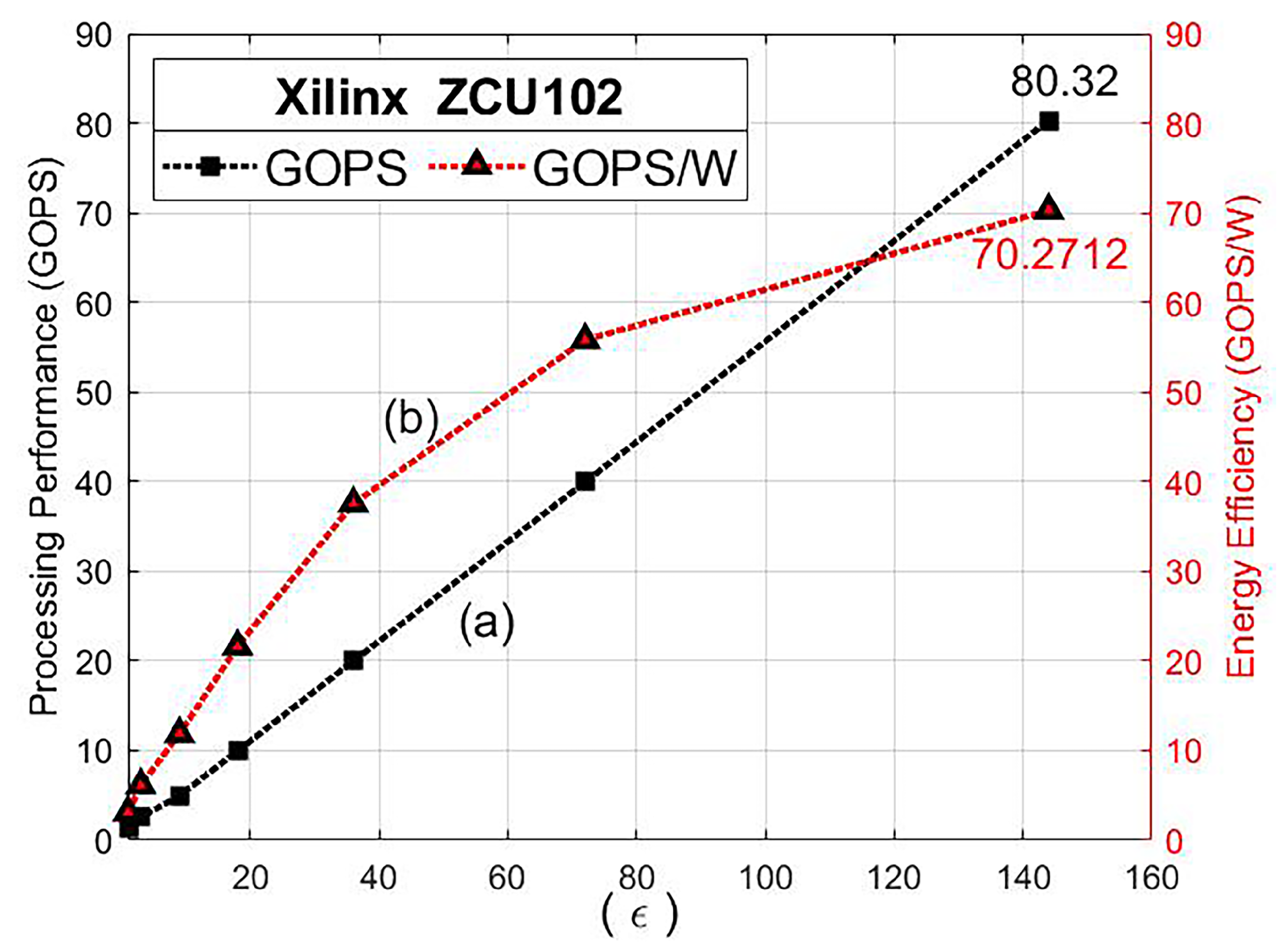
3.4. Design Space Exploration

Among various FPGA devices, the density of their processing resources available, such as DSPs, BRAMs, LUTs, and Flip-Flops, differs in combinations. The number of DSP blocks and BRAM banks required is predicted in Section 3.2 and  Section 3.3, respectively. Notably, the bandwidth bottleneck emerges when the data processing time is not well matched to that of the data transfer, hence compromising the peak performance. In the design space specified by the FPGA device parameters, we need to find ways of acquiring optimal solutions under the constraints of the algorithm parameters.

Balancing between the computation and the transfer times is considered in this paper as well, especially when it is taken to process C channels of W×(n+1)inFMs and finally output 2W×2m outFMs, as expressed in Equations (10)–(12).

$$\left\{\begin{array}{c}{T}_{i\_transfer}=\frac{16\times (m+1)\times W\times C}{AchievedBandwidth}\hfill \\ T_{o\_transfer}=\frac{16\times 2m\times 2W\times N}{AchievedBandwidth}\hfill \\ T_{f\_transfer}=\frac{16\times C\times N\times K^2}{AchievedBandwidth}\hfill \end{array}\right.$$

(10)

$$T_{transfer}=T_{i\_transfer}+T_{o\_transfer}+T_{f\_transfer}$$

(11)

Here, $T_{i\_transfer}$, $T_{o\_transfer}$, and $T_{f\_transfer}$ are the respective transferring times of the inFMs, outFMs, and filters. Bandwidth is the device constraint provided by FPGA.

$$T_{computer}=\left(⌈\frac{W}{m+1}⌉\times ⌈\frac{C}{{\mathrm{P}}_{\mathrm{C}}}⌉\times ⌈\frac{N}{{\mathrm{P}}_{\mathrm{N}}}⌉\times I{I}_{PU}+I{L}_{PU}\right)\times 1/\phantom{1freq}freq$$

(12)

where ${\mathit{II}}_{PU}$ and ${\mathit{IL}}_{PU}$ are characterized in Equation (6).

Our goal is to find the minimal $T_{computer}$ under the premise of $T_{computer}$≥$T_{transfer}$ since the peak performance must match the bandwidth. {$P_C$, $P_N$, $\epsilon$, m} are unknown parameters to be explored. In Equation (6), ${\mathit{II}}_S$ and ${\mathit{IL}}_S$ can be obtained via a few small-scale experiments. {W, C, N, K} are parameters relevant to the transposed convolution while {freq, Achieved, and Bandwidth} are related to the FPGA hardware. In this paper, Algorithm 1 is devised to explore the optimal solution of {$P_C$, $P_N$, $\epsilon$, m} based on the above analysis.

Algorithm 1$:\mathbf{Design}\mathbf{space}\mathbf{exploration}$.

Require: $T:\left\{WCKN\right\}$,      $F:\left\{freqAchievedBandwidthI{I}_{s}I{L}_s\right\}$,      $F:\left\{AvailableDSPAvailableBRAM\right\}$ Ensure: {P${}_C$  P${}_N$   $\epsilon$   m} functionExplore_minTime($T,F$)   $init{T}_{min}=ANumberLargeEnough$   $initOptimization\_parameter\left[\right]=\{0,0,0,0\}$   $init\epsilon \_table\left[2\right]\left[\right]=\left\{\right\{144,72,36,18,9,3\},\{64,32,16,8,4,2\left\}\right\}$   $initm\_map\left[2\right]=\{4,2\}$   for each $indexin\{0,1\}$ do     $m\leftarrow m\_map\left[index\right]$     $I{N}_{buffer}\leftarrow (m+n+2)\times (m+1)$     $OU{T}_{buffer}\leftarrow 8(m\times m)$     $FILTE{R}_{buffer}\leftarrow 2(K\times K)$     for $each{\epsilon }_{i}in\epsilon \_table\left[index\right]$ do       $P_C{P}_N$←$\lfloor \frac{AvailableDSPBlocks}{{\epsilon }_i}\rfloor$       for each pair of {P${}_C$,P${}_N$} in results of Factorization(P${}_C$P${}_N$) do         if $P_C\times I{N}_{buffer}+P_N\times OU{T}_{buffer}+P_C\times P_N\times FILTE{R}_{buffer}$                           $<=$$AvailableBRAM$ then           $T_{computer}\leftarrow Equation\left(6\right)\left(12\right)$           $T_{transfer}\leftarrow Equation\left(10\right)\left(11\right)$           if $T_{computer}<=T_{transfer}$ then             $T_{computer}\leftarrow T_{transfer}$           end if           $T_{total\_computer}\leftarrow T_{computer}\times \lceil \frac{H}{m+1}\rceil$           if $T_{total\_computer}<T_{min}$ then             $T_{min}\leftarrow T_{total\_computer}$             $Optimization\_parameter\leftarrow \left\{P_C{P}_N\epsilon m\right\}$           end if         end if       end for     end for   end for   return $Optimization\_parameter$ end function

4. Experiment Verification

4.1. Experimental Cases for GANs

The design configurations for some of its transposed convolution layers regarding seven typical GAN models are listed in

Table 4. Design configurations of GANs.

GANs	Transposed Convolution Layers			GANs	Transposed Convolution Layers
	#num	input	filters		#num	input	filters
	#2	4×4×1024	5×5×1024×512		#2	4×4×512	4×4×512×256
DCGAN [4]	#3	8×8×512	5×5×512×256	GP-GAN [7]	#3	8×8×256	4×4×256×128
	#4	16×16×256	5×5×256×128		#4	16×16×128	4×4×128×64
	#5	32×32×128	5×5×128×3		#5	32×32×64	4×4×64×3
	#2	4×4×1024	4×4×1024×512		#2	4×4×4×512	4×4×4×512×256
Disco-GAN [5]	#3	8×8×512	4×4×512×256	3D-GAN [10]	#3	8×8×8×256	4×4×4×256×128
	#4	16×16×256	4×4×256×128	3D-ED-GAN [9]	#4	16×16×16×128	4×4×4×128×64
	#6	32×32×128	4×4×128×3		#5	32×32×32×64	4×4×4×64×1
	#2	4×4×512	4×4×512×256		#2	4×4×2048	4×4×2048×1024
	#3	8×8×256	4×4×256×128		#3	8×8×1024	4×4×1024×512
Art-GAN [6]	#4	16×16×128	4×4×128×128	EB-GAN [8]	#4	16×16×512	4×4×512×256
	#6	16×16×128	4×4×128×3	(256×256 model	#5	32×32×256	4×4×256×128
				on IMAGENET)	#6	64×64×128	4×4×128×64
					#7	128×128×64	4×4×64×64

. In the table, the label #num denotes an order of the layer in the network. For networks such as DCGAN [4], Disco-GAN [5], Art-GAN [6], GP-GAN [7], and EB-GAN [8], they are mainly applied for the purpose of synthesizing images, while the others such as 3D-ED-GAN [9] and 3D-GAN [10] fulfill the tasks of generating 3D object.

4.2. Experimental Setup

To evaluate our design approach, those state-of-the-art transposed convolution layers of GANs were tested on the Xilinx FPGA platform with Vivado HLS (v2018.2). HLS provides abundant optimization directives for pipeline, parallelism, and memory partition by adding #pragma to the C/C++ code. The RTL representation of the design in terms of the Verilog HDL code can be exported as a Vivado’s IP core after running C Synthesis and C/RTL Co-simulation. Finally, the Vivado Tool synthesizes the exported RTL codes and records the design specifics in the report file. In addition, the XPower analyzer tool integrated into Vivado performs the power estimation. Two Xilinx devices were adopted in this experiment: XCZU9EG and XC7Z045. They were integrated into the ZCU102 board and ZC706 board, respectively, together with the ARM core, and offer high-speed serial connectivity taking advantage of integrated AXI IP.

We implemented the networks in Table 4 using our techniques.

Table 5. Parameters for devices.

Device	$\left(\mathit{\epsilon }\right)$	m	${\mathit{P}}_{\mathit{C}}$×${\mathit{P}}_{\mathit{N}}$
XCZU9EG	144	4	16
XC7Z045	144	4	4

delivers the parameters for FPGA devices in our implementations.

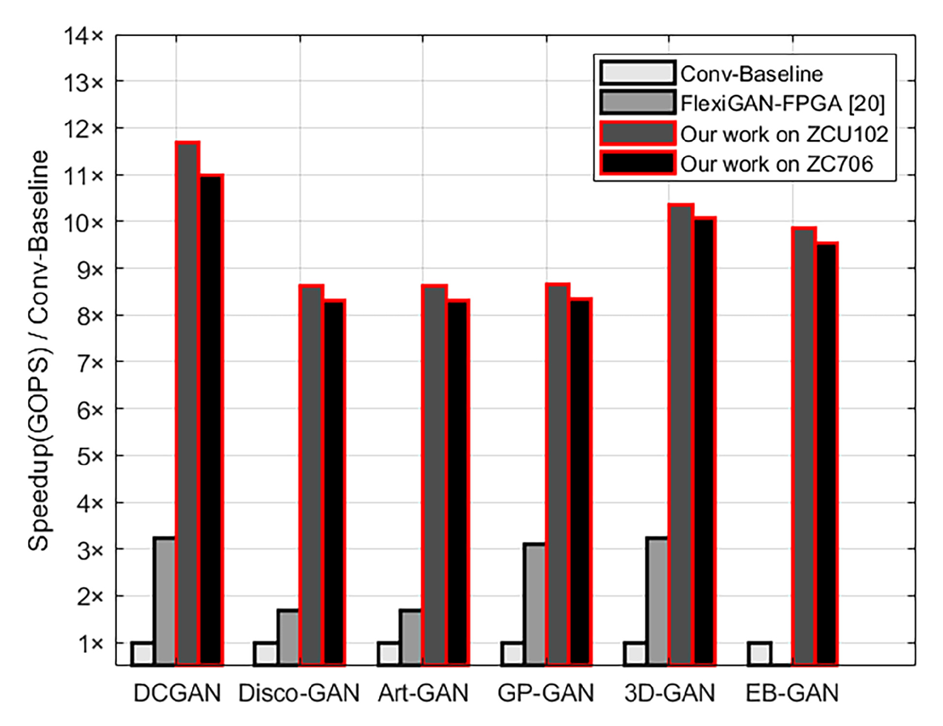
4.3. Experimental Results

In this subsection, our experimental results are reported. We adopt the previous view [18] about the computation means of GOP of transposed convolution. Therefore, the processing capability of our implementation is defined by Equation (13):

$$GOPS=\frac{2\times C\times W\times H\times N\times K^2}{T_{prepare}+T_{total\_computer}}$$

(13)

where $T_{prepare}$ denotes the time of loading the first (n+1) rows of inFMs and the first batch of filters into on-chip BRAM banks.

Table 6. Performance and resource report.

GAN Models	Layers	Performance (GOPS)		GAN Models	Layers	Performance (GOPS)
		ZCU102	ZC706			ZCU102	ZC706
	#2	717.2	223.7		#2	406.8	136.6
	#3	915.9	243.4	3D-GAN [10]	#3	536.4	151.3
DCGAN [4]	#4	1058.7	254.3	3D-ED-GAN [9]	#4	627.9	159.1
	#5	320.2	133.8		#5	213.7	87.5
	avg	851.8	236.9		avg	482.4	142.8
	#2	544.9	152.1		#2	654.9	161.1
	#3	651.8	161.2		#3	727.1	166.3
Disco-GAN [5]	#4	719.4	165.5	EB-GAN [8]	#4	768.5	168.5
	#6	252.1	94.5	(256×256 model	#5	789.1	169.6
	avg	616.1	157.6	on IMAGENET)	#6	795.9	170.2
Art-GAN [6]	#2	406.8	136.6		#7	805	170.5
	#3	536.4	151.3		avg	759.9	168.2
	#4	627.9	159.1	Freq (MHz)		200	167
	#6	213.7	87.5	LUT Utilization (%)		97	90
	avg	486.9	145.4	DSP Utilization (%)		91.4	67
GP-GAN [7]	#2	406.8	136.6	BRAM Utilization (%)		90	57
	#3	536.4	151.3	Performance (GOPS)		639.2*(avg)	162.5*(avg)
	#4	627.9	159.1	DSP Efficiency (GOPS/DSP)		0.254${}^{♯}$(avg)	0.181${}^{♯}$(avg)
	#5	213.7	87.5	Power (W)		15.6	5.8
	avg	486.9	145.4	Energy Efficiency (GOPS/W)		40.9	27.9

shows the experimental results in terms of performance and power as well as resource utilization. We also provide avg GOPS and avg DSP Efficiency. In

Table 7. Comparison to prior implementations.

Models	Works	Device	Precision	DSP	Freq	GOPS	GOPS/DSP
AlexNet [21]	[13]	VX485T	float	2800	100	61.62	0.022
(Convolution)	[23]	ZC706	16 fixed	900	167	271.8	0.224
		ASIC	8 fixed			409.6
	GAN [17]	(TSMC	16×8 fixed		200	204.8
Transposed		28 nm)	16 fixed			102.4
Convolution	[18]	7Z020	12 fixed	220	100	2.6	0.012
	Ours	ZCU102	16 fixed	2520	200	639.2 *	0.245 ${}^{♯}$
	Ours	ZC706	16 fixed	900	167	162.5 *	0.181 ${}^{♯}$
* Our avg GOPS = The total GOP of GANs in Table 4/The total time occupation
${}^{♯}$ Our avg GOP/DSP = The total GOP of GANs in Table 4 /the total time occupation/DSPs

, we compare the prior implementations, showing that our accelerator yields 15× (up to 21×) increase in DSP efficiency over prior work [18]. Actually, neither the work of Zhang [18] nor GNA [17] implements real-life GAN models. Moreover, GNA’s partial study on transposed convolution layers focuses on the bit-width flexibility optimization based on TSMC 28nm ASIC. The meanings of GOPS given by Lu [23] and Zhang [13] differ from ours since they implemented the general convolutional neural network called AlexNet [29].

To further compare with prior work that implements real-life GAN models, we directly mapped the transposed convolution to general convolution utilizing the optimized FPGA-based conventional accelerator as the baseline, which is the same as that employed by FlexiGAN-FPGA [20]. Figure 14 records the speedup (GOPS) with our work and prior work [20] vs. Conv-baseline separately. We produce 8.6× (up to 11.7×) improvement in processing throughput over the Conv-baseline.

5. Conclusions

To address the two issues of having ineffective operations and being computationally intensive inherently when implementing transposed convolution layers of GANs on FPGAs, we present the novel Wino-transCONV dataflow as well as its corresponding hardware architecture design. In this work, the distinct memory partition technique and the hardware-based design space are also explored. Our final implementations of seven state-of-the-art GANs achieve an overall performance of 639.2 GOPS on the Xilinx ZCU102 platform and 162.5 GOPS on the VC706 platform. The experiment results also show that our accelerator design yields 21× improvement in DSP efficiency over other prior works. In addition, in comparison to the best-known work, which delivers 2.2× higher performance than the optimized conventional accelerator baseline, the proposed design achieves 8.6× (up to 11.7×) increase in processing throughput over the Conv-baseline.

References

1. Zhang, Y.; Pezeshki, M.; Brakel, P.; Zhang, S.; Laurent, C.; Bengio, Y.; Courville, A. Towards End-to-End Speech Recognition with Deep Convolutional Neural Networks. In Proceedings of the International Symposium on Computer Architecture (ISCA), Seoul, Korea, 8–22 June 2016; pp. 410–414. [Google Scholar]
2. Goodfellow, I.J.; Pouget-Abadie, J.; Mirza, M.; Xu, B.; Warde-Farley, D.; Ozair, S.; Courville, A.; Bengio, Y. Generative Adversarial Networks. Adv. Neural Inf. Process. Syst. 2014, 3, 2672–2680. [Google Scholar]
3. Mirza, M.; Osindero, S. Conditional Generative Adversarial Nets. arXiv 2014, arXiv:1411.1784. [Google Scholar]
4. Radford, A.; Metz, L.; Chintala, S. Unsupervised representation learning with deep convolutional generative adversarial networks. arXiv 2015, arXiv:1511.06434. [Google Scholar]
5. Taeksoo, K.; Moonsu, C.; Hyunsoo, K.; Lee, J.K.; Kim, J. Learning to discover cross-domain relations with generative adversarial networks. In Proceedings of the 34th International Conference on Machine Learning (ICML), Sydney, Australia, 6–11 August 2017; Volume 70, pp. 1857–1865. [Google Scholar]
6. Tan, W.R.; Chan, C.S.; Aguirre, H.E.; Tanaka, K. ArtGAN: Artwork synthesis with conditional categorical GANs. In Proceedings of the 2017 IEEE International Conference on Image Processing (ICIP), Beijing, China, 17–20 September 2017; pp. 3760–3764. [Google Scholar]
7. Wu, H.; Zheng, S.; Zhang, J.; Huang, K. GP-GAN: Towards Realistic High-Resolution Image Blending. In Proceedings of the 27th ACM International Conference on Multimedia (ACMMM), Nice, France, 21–25 October 2019; Association for Computing Machinery: New York, NY, USA, 2019; pp. 2487–2495. [Google Scholar]
8. Zhao, J.; Mathieu, M.; Lecun, Y. Energy-based Generative Adversarial Network. In Proceedings of the 5th International Conference on Learning Representations (ICLR), Toulon, France, 24–26 April 2017; pp. 100–109. [Google Scholar]
9. Wang, W.; Huang, Q.; You, S.; Yang, C. Ulrich Neumann. Shape Inpainting Using 3D Generative Adversarial Network and Recurrent Convolutional Networks. In Proceedings of the 2017 IEEE International Conference on Computer Vision (ICCV), Venice, Italy, 22–29 October 2017; pp. 2317–2325. [Google Scholar]
10. Wu, J.; Zhang, C.; Xue, T.; Freeman, B.; Josh, T. Learning a Probabilistic Latent Space of Object Shapes via 3D Generative-Adversarial Modeling. In Proceedings of the Conference and Workshop on Neural Information Processing Systems (NIPS), Barcelona, Spain, 5–10 December 2016; pp. 82–90. [Google Scholar]
11. Wei, W.; Yu, C.H.; Zhang, P.; Chen, P.; Wang, Y.; Hu, H.; Liang, Y.; Cong, J. Automated Systolic Array Architecture Synthesis for High Throughput CNN Inference on FPGAs. In Proceedings of the 2017 54th ACM/EDAC/IEEE Design Automation Conference (DAC), Austin, TX, USA, 18–22 June 2017; pp. 1–6. [Google Scholar]
12. DiCecco, R.; Lacey, G.; Vasiljevic, J.; Chow, P.; Taylor, G.; Areibi, S. Caffeinated FPGAs: FPGA Framework for Convolutional Neural Networks. In Proceedings of the 2016 International Conference on Field-Programmable Technology (FPT), Xi’an, China, 7–9 December 2016; pp. 265–268. [Google Scholar]
13. Zhang, C.; Li, P.; Sun, G.; Guan, Y.; Xiao, B.; Cong, J. Optimizing fpga-based accelerator design for deep convolutional neural networks. In Proceedings of the 2015 ACM/SIGDA International Symposium on Field-Programmable Gate Arrays, Monterey, CA, USA, 22–24 February 2015; ACM: New York, NY, USA, 2015; pp. 161–170. [Google Scholar]
14. Ma, Y.; Cao, Y.; Vrudhula, S.; Seo, J. Optimizing the Convolution Operation to Accelerate Deep Neural Networks on FPGA. IEEE Trans. Very Large Scale Integr. Syst. 2018, 26, 1354–1367. [Google Scholar] [CrossRef]
15. Chen, T.; Du, Z.; Sun, N.; Wang, J.; Wu, C.; Chen, Y.; Temam, O. A High-Throughput Neural Network Accelerator. IEEE Micro 2019, 35, 24–32. [Google Scholar]
16. Liu, Z.; Chow, P.; Xu, J.; Jiang, J.; Dou, Y.; Zhou, J. A Uniform Architecture Design for Accelerating 2D and 3D CNNs on FPGAs. Electronics 2019, 8, 65. [Google Scholar] [CrossRef] [Green Version]
17. Yan, J.; Yin, S.; Tu, F.; Liu, L.; Wei, S. GNA: Reconfigurable and Efficient Architecture for Generative Network Acceleration. IEEE Trans. Comput.-Aided Des. Integr. Circuits Syst. 2018, 37, 2519–2529. [Google Scholar] [CrossRef]
18. Zhang, X.; Das, S.; Neopane, O.; Kreutz-Delgado, K. A Design Methodology for Efficient Implementation of Deconvolutional Neural Networks on an FPGA. arXiv 2017, arXiv:1705.02583. [Google Scholar]
19. Yazdanbakhsh, A.; Falahati, H.; Wolfe, P.J.; Samadi, K.; Kim, N.S.; Esmaeilzadeh, H. GANAX: A unified MIMD-SIMD acceleration for generative adversarial networks. In Proceedings of the 2018 ACM/IEEE 45th Annual International Symposium on Computer Architecture (ISCA), Los Angeles, CA, USA, 2–6 June 2018; pp. 650–661. [Google Scholar]
20. Yazdanbakhsh, A.; Brzozowski, M.; Khaleghi, B.; Ghodrati, S.; Samadi, K.; Kim, N.S.; Esmaeilzadeh, H. FlexiGAN: An End-to-End Solution for FPGA Acceleration of Generative Adversarial Networks. In Proceedings of the 2018 IEEE 26th Annual International Symposium on Field-Programmable Custom Computing Machines (FCCM), Boulder, CO, USA, 29 April–1 May 2018; pp. 65–72. [Google Scholar]
21. Chang, J.W.; Kang, K.W.; Kang, S.J. An Energy-Efficient FPGA-based Deconvolutional Neural Networks Accelerator for Single Image Super-Resolution. IEEE Trans. Circuits Syst. Video Technol. 2020, 30, 281–295. [Google Scholar] [CrossRef] [Green Version]
22. Chen, Y.-H.; Krishna, T.; Emer, J.S.; Sze, V. Eyeriss: An Energy-Efficient Reconfigurable Accelerator for Deep Convolutional Neural Networks. IEEE J. Solid-State Circuits 2017, 52, 127–138. [Google Scholar] [CrossRef] [Green Version]
23. Lu, L.; Liang, Y.; Xiao, Q.; Yan, S. Evaluating Fast Algorithms for Convolutional Neural Networks on FPGAs. In Proceedings of the 2017 IEEE 25th Annual International Symposium on Field-Programmable Custom Computing Machines (FCCM), Napa, CA, USA, 30 April–2 May 2017; pp. 101–108. [Google Scholar]
24. Aydonat, U.; O’Connell, S.; Capalija, D.; Ling, A.C.; Chiu, G.R. An OpenCL™ Deep Learning Accelerator on Arria 10. In Proceedings of the ACM/SIGDA International Symposium on Field-Programmable Gate Arrays (FPGA), Monterey, CA, USA, 22–24 February 2017; pp. 55–64. [Google Scholar]
25. Lavin, A.; Gray, S. Fast Algorithms for Convolutional Neural Networks. In Proceedings of the 2016 IEEE Conference on Computer Vision and Pattern Recognition (CVPR), Las Vegas, NV, USA, 27–30 June 2016; pp. 4013–4021. [Google Scholar]
26. Guo, K.; Zeng, K.; Yu, J.; Wang, Y.; Yang, H. A Survey of FPGA Based Neural Network Accelerator. arXiv 2017, arXiv:1712.08934. [Google Scholar]
27. Xilinx, Inc. UG871-Vivado High Level Synthesis Tutorial; Xilinx: San Jose, CA, USA, 3 April 2013; pp. 120–130. [Google Scholar]
28. Xilinx, Inc. UG902 Vivado High Level Synthesis; Xilinx: San Jose, CA, USA, 20 December 2018; pp. 6–8. [Google Scholar]
29. Krizhevsky, A.; Sutskever, A.; Hinton, G.E. ImageNet Classification with Deep Convolutional Neural Networks. In Proceedings of the 25th International Conference on Neural Information Processing Systems (NIPS), Lake Tahoe, NV, USA, 3–8 December 2012; pp. 1097–1105. [Google Scholar]
Figure 1. DCGAN: An actual GAN generator for LSUN scene modeling.
Electronics 09 00286 g001
Figure 2. Data processing flow of transposed convolution layer.
Electronics 09 00286 g002
Figure 3. An illustration of the data transformation flow through inserting and padding with zeros.
Electronics 09 00286 g003
Figure 4. An illustration of picking the effective filter values in alignment to the non-zero grids in inFM.
Electronics 09 00286 g004
Figure 5. An illustration to the data operations in dissolving a transposed convolution into four equivalent convolutions during the DECOMPOSITION processing.
Electronics 09 00286 g005
Figure 6. The data REARRANGEMENT process.
Electronics 09 00286 g006
Figure 7. An algorithmic chart for the proposed Wino-transCONV dataflow.
Electronics 09 00286 g007
Figure 8. An illustration of the Wino-transCONV design architecture.
Electronics 09 00286 g008
Figure 9. The architecture-to-implementation mapping on FPGA for a PU.
Electronics 09 00286 g009
Figure 10. Design of processing unit.
Electronics 09 00286 g010
Figure 11. Timing diagrams of four typical parallel implementations for S1–S5 operations in a PU.
Electronics 09 00286 g011
Figure 12. Characterization of performance vs. ε for a PU design.
Electronics 09 00286 g012
Figure 13. An illustration of memory partition.
Electronics 09 00286 g013
Figure 14. Comparison between our work and the prior work [20] on the speedup ratio against Conv-Baseline.
Electronics 09 00286 g014