A Detection Approach Using LSTM-CNN for Object Removal Caused by Exemplar-Based Image Inpainting

1
Beijing Key Lab of Intelligent Telecommunication Software and Multimedia, Beijing University of Posts and Telecommunications, Beijing 100876, China
2
School of Computer Science and Software Engineering, University of Science and Technology Liaoning, Anshan 114051, China
*
Authors to whom correspondence should be addressed.
Electronics 2020, 9(5), 858; https://0-doi-org.brum.beds.ac.uk/10.3390/electronics9050858
Submission received: 29 April 2020
/
Revised: 14 May 2020
/
Accepted: 20 May 2020
/
Published: 22 May 2020
(This article belongs to the Section Computer Science & Engineering)
Abstract
:Exemplar-based image inpainting technology is a “double-edged sword”. It can not only restore the integrity of image by inpainting damaged or removed regions, but can also tamper with the image by using the pixels around the object region to fill in the gaps left by object removal. Through the research and analysis, it is found that the existing exemplar-based image inpainting forensics methods generally have the following disadvantages: the abnormal similar patches are time-consuming and inaccurate to search, have a high false alarm rate and a lack of robustness to multiple post-processing combined operations. In view of the above shortcomings, a detection method based on long short-term memory (LSTM)-convolutional neural network (CNN) for image object removal is proposed. In this method, CNN is used to search for abnormal similar patches. Because of CNN’s strong learning ability, it improves the speed and accuracy of the search. The LSTM network is used to eliminate the influence of false alarm patches on detection results and reduce the false alarm rate. A filtering module is designed to eliminate the attack of post-processing operation. Experimental results show that the method has a high accuracy, and can resist the attack of post-processing combination operations. It can achieve a better performance than the state-of-the-art approaches.
1. Introduction
1.1. Motivation
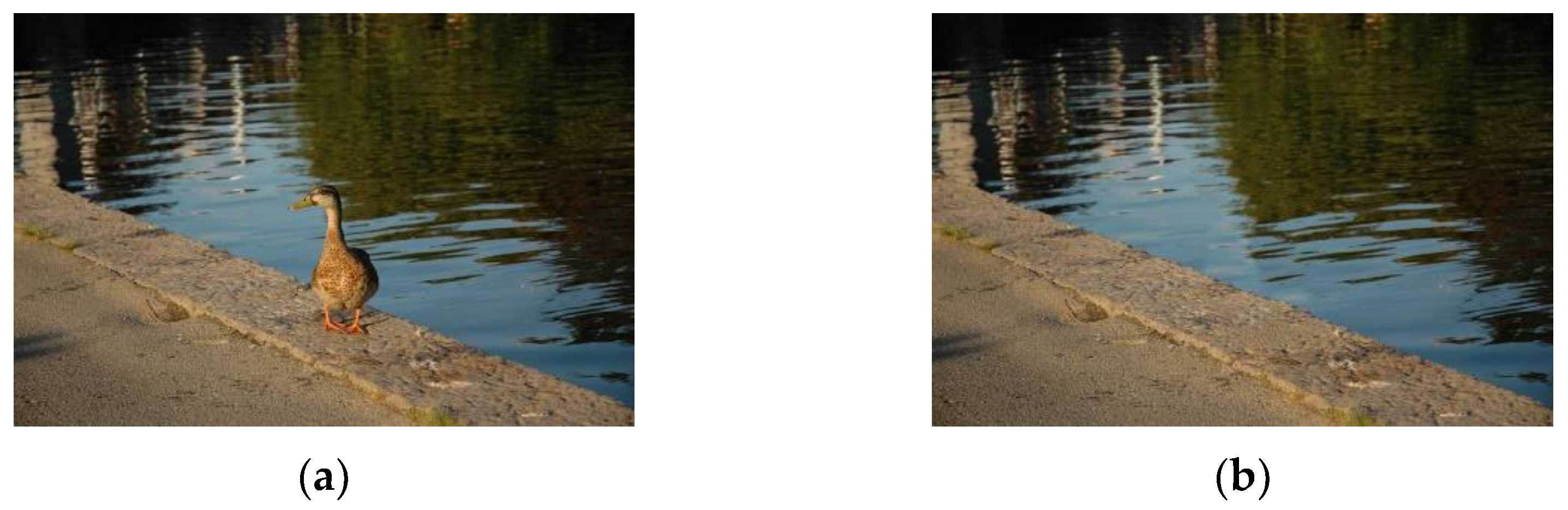
Image inpainting is a new image processing algorithm, which has been studied deeply by many scholars. Inspired by the real painting restoration technology, a method of image inpainting based on image patches copy and paste is proposed by Criminisi et al. [1], which can effectively inpaint the damaged or removed image regions in a visually reasonable way, using the information preserved in the surrounding regions. As an important subject in the field of computer vision and image processing, image inpainting has made great progress in recent years, and plays an important role in image restoration [2], image coding and transmission, image editing [3]. However, image inpainting can also be used to tamper with image content maliciously, which provides a useful tool for object removal, and brings the trust crisis to image content [1]. Object removal achieved by image inpainting leaves no obvious visually traces of tampering, which can simultaneously maintain texture and structure consistency [4]. As a result, it makes passive image forensics extremely challenging. For example, in Figure 1, the duck is removed from the original image by image inpainting, and then the inpainted image is processed by post-processing operation, such as JPEG compression, which not only changes the semantic information of image, but also causes a loss of forensic information, thus increasing the difficulty of image forensics.
1.2. Related Work
There are few existing researches on passive blind forensics of digital image inpainting. Wu et al. [5] took the lead in proposing a passive forensics algorithm to distinguish between a natural image and an inpainted image. This method uses zero-connectivity features to screen out suspicious regions, and computed fuzzy membership between similar patches to identify tampered regions. However, the suspicious regions need to be manually selected in advance, resulting in low efficiency and high false alarm rate. In addition, the algorithm uses full search to find suspicious patches, which leads to high computational complexity. Bacchuwar et al. [6] proposed an improved algorithm based on skip block matching; compared with the algorithm in reference [5], the computational costs are obviously reduced, but the detection regions still need to be selected manually, so it is still a semi-automatic method. In addition, all of the above algorithms produce serious false detection for the sky, grassland and other texture consistent regions in the image background. To overcome the drawbacks of the above methods, a two-stage searching forensics algorithm based on multi-region relations is proposed by Chang et al. [7]. This method uses vector filtering to remove false alarm blocks in the uniform background, multi-region relations, to identify tampered blocks and the mapping method based on weight transformation to speed up the search of suspicious blocks. It improves the false-alarm performance and calculation efficiency, but it limits the further improvement of search speed and detection accuracy. Liang et al. [8] proposed a fast search algorithm using central pixel mapping to search suspicious areas; the detection algorithm was further optimized and the search speed was improved. However, this method is not universal and cannot be applied to the detection of all image inpainting forgery methods. In addition, the forger can further hide the tampering trace of image inpainting through some post-processing technologies, which makes forensic work more complex. Although a few detection methods increase the resistance to the attack of post-processing, they have some limitations and shortcomings. The method [9] detects the forgery operation of the compressed inpainted image, by computing and segmenting the averaged sum of absolute difference between the forged image and the JPEG compressed image with different quality factors. In reference [10], a large feature mining method based on discrete transform domain is proposed. In order to prevent from the overfitting of classifiers under high feature dimension, this method applies ensemble learning to deal with the problem of high feature dimension, exposes inpainting forgery under post recompression attacks. However, these two methods [9,10] are only suitable for JPEG image compression attack, not for other post-processing operations. Although reference [11] proposed the detection method of image inpainting forgery, which can resist post-processing attacks such as JPEG compression and Gaussian noise to some extent, it is unable locate the tampered region of the image. Therefore, almost none of the existing methods can resist a variety of post-processing attacks, and accurately locate the tampered region for the detection of image inpainting, simultaneously.
1.3. Main Contribution
In order to make up for the shortcomings of existing methods in the images inpainting forensics, reveal the image inpainting with post-processing attacks, this paper proposes an image inpainting forensics method based on long short-term memory (LSTM)-convolutional neural network (CNN), which uses a convolutional neural network (CNN) to identify suspicious similar patches in the tampered image, and exploits LSTM to distinguish the texture consistent regions from suspicious regions, so as to greatly reduce the false alarm rate. In order to resist post-processing attacks effectively, this paper designed a filter module to eliminate the disturbances caused by the post-processing operations for the detection of image inpainting.
The main contributions of this paper are as follows:
- We present a CNN based nearest neighbor image patch matching algorithm to quickly search for abnormal similar patches in images;
- We design a false alarm removal module based on the CNN and LSTM network. In this module, CNN and LSTM are combined to identify the normal texture consistent area in the image, and then remove the false alarm patches from the suspicious patches;
- We present a post-processing feature filtering algorithm. In the detection of tampered images, the CNN network is more focused on learning the trace features introduced by image tampering;
- The LSTM-CNN network, based on the encoder-decoder architecture for image inpainting forensics, is proposed in this paper.
The article has been organized in the following way: the research motivation, related work and the main contributions are introduced in Section 1. Section 2 describes the background knowledge of image inpainting. Section 3 gives the solution of key problems in image inpainting forensics. The LSTM-CNN network for image inpainting forensics is described in Section 4. In Section 5, a series of experiments are designed to verify the effectiveness of the proposed detection method. Finally, the work is concluded in Section 6.
2. Background
The existing image inpainting methods can be roughly divided into two categories: one is the method based on diffusion; the other is the method based on exemplar. The former solves the partial differential equation describing diffusion, so as to diffuse the information of known regions to the damaged or removed regions [12,13,14,15]. However, they do not perform well in inpainting regions with complex texture or large regions; it is not suitable for large object removal from images. The latter propagates the known exemplars to the missing patches gradually. In order to produce better inpainting effect for large missing regions, exemplar priority is defined to encourage inpainting on the structure. The method can also be used to remove object in the image, so as to tamper with the image. It is the main focus of image forensics in this paper.
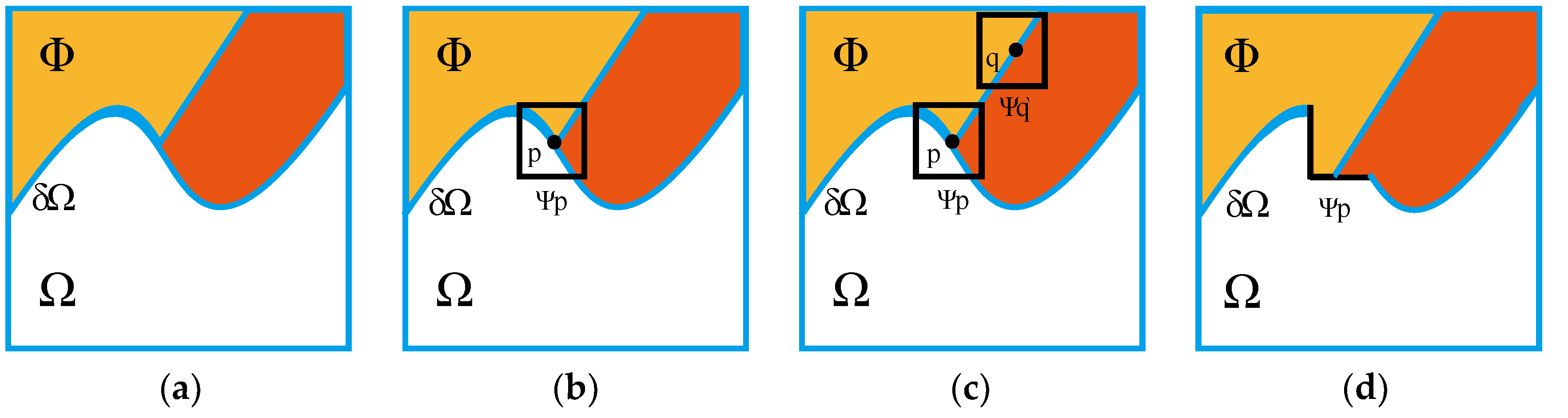
The classic algorithm of image inpainting based on exemplar is Criminisi’s algorithm. At present, most of the image inpainting algorithms are improved in Criminisi’s algorithm, such as the algorithms in reference [16,17]. The following is an example of Criminisi’s algorithm to illustrate its inpainting process, as shown in Figure 2, in which Ω is the region to be inpainted, δΩ is the boundary of region to be inpainted, and Φ is the known complete region without missing information in the image. The specific steps of Criminisi’s algorithm are as follows:
Step 1: The priority for each point on δΩ is calculated to get the point p with the highest priority, and then select the image patch Ψp centered at the point p as the current patch to be inpainted, as shown in Figure 2b. For any patch Ψp centered at the point p, where p ∈ δΩ, its priority P(p) will be defined as the product of two items, as in Equation (1):
P(p) = C(p) D(p)
C(p) is the confidence term and D(p) is the data term, defined as follows:
where |Ψp| denotes the area of patch Ψp, α is the normalization factor, np is the unit orthogonal vector, and ┴ is the orthogonal operator.
Step 2: Search the image patch Ψq` which is most similar to Ψp in the known image region Φ, as shown in Figure 2c. The measure of similarity between patches follows Equation (4):
where d (Ψp`, Ψq) is the distance between two patches, and Ψp` is the patch with the highest priority.
Step 3: The missing region in Ψp is filled by the pixels at the corresponding position in the best matching patch Ψq`. Then, the boundary δΩ and the confidence term C(p) are updated by new Ψp`, as shown in Figure 2d. The update rule of C(p) conforms to the following Equation (5):
C(p)` is the confidence value which has been updated.
Step 4: Repeat the above steps, until the region to be inpainted is filled completely.
The Criminisi’s algorithm can keep the image structure and texture consistent when inpainting the damaged area; it is difficult to find traces with the naked eye. It brings the performance advantage to Criminisi’s algorithm. There are a few improved inpainting algorithms [16,17,18] proposed based on the main idea of Criminisi’s algorithm, which only focus on improving priority calculation and optimizing search strategy. However, Criminisi’s algorithm and its improved algorithm are not invulnerable. While maintaining both perception quality and efficiency well, they introduce the abnormal similarity between the best matching patch and the filled patch. Although there are also a lot of irregular patches in normal images that look the same or similar, there are actually subtle differences. It provides a useful clue for the detection of image inpainting.
3. The Solutions to Key Problems
According to the existing image inpainting forensics methods, the process of image inpainting forensics is roughly as follows: first, according to certain patch matching rules (such as Euclidean distance), the whole image is searched to find the best matching patch for each patch in the image. Then, between the matching patches, the patch features reflecting the inpainting information is extracted. Next, the classification rule (such as a fuzzy membership function) is exploited; the pixels of patch are divided into the inpainted set and the uninpainted set. Finally, in order to reduce the false alarm rate, the correction is performed in combination with the observation of the false alarm area.
Through the in-depth analysis of the existing methods for image inpainting forensics, we find that they have the following common shortcomings:
- (1)
- Due to the need of similarity measurement between any two patches in the whole image, the search for similar patches is very time-consuming, especially for large images.
- (2)
- The detection of image inpainting only depends on finding the abnormal similarity of patches. In a normal image, there are some very similar patches (such as blue sky, grassland and other uniform regions), although there are still differences in the details. However, it is very easy to be confused in the actual feature classification, and it is difficult to correctly identify the classification of pixels in such kinds of patches.
- (3)
- There is no robust and effective forensics method for image inpainting with multiple post-processing combined operations.
In view of the above shortcomings, this paper proposes the solutions to these key problems for the detection of exemplar-based image inpainting.
3.1. The Search of Abnormal Similar Patches
In order to search the abnormal similar patches in the image, the reference patch and the target patch must be determined. Since the specific location of image inpainting is not known at first, the easiest way is to select the reference patch randomly from the training image through an exhaustive search. In order to reduce the computation, we propose a CNN based nearest neighbor image patch matching algorithm to quickly search for abnormal similar patches in images. The general idea of the algorithm: firstly, the selected reference patch in the input image is given a label, and the label of patch Ψp is defined as Equation (6):
where Ψp is any patch, and
is the selected reference patch in the image. When patch Ψp is selected as the reference patch, the label value is 1, otherwise, it is 0. When the label value of a reference patch is 1, in a search for the target patch around the reference patch, the similarity between pixels is calculated by using the hidden layer [19], and the similarity between pixels is measured by Euclidean distance, as shown in Equation (7):
where f (x) represents the pixel strength of the target patch, and f (x0) represents the pixel strength of the reference patch. According to Equation (7), when the target patch is the most similar to the selected reference patch, the algorithm updates the reference patch through the label value and the central pixel of reference patch, and the update way adopts the propagation. The specific steps are as follows:
Ec (f(x), f(x0)) = ||f(x) − f(x0)||22
- (1)
- The nearest neighborhood patch is defined as the function f: A→R2, where A represents the reference patch, and R is the offset between the possible nearest neighborhood patches (with the center of patch as the reference).
- (2)
- For the selected reference patch, check the nearest neighborhood patch and its corresponding relationship. If the nearest neighbor patch produces the best similarity value, the corresponding benchmark of the reference patch is updated through the activation function [20]. Assuming that a reference patch centered at the pixel p(x, y) is selected, propagation starts from the neighborhood patch to search for the current match; for example, q = (x + R, y + R) ↔ s = (i, j, k), where (i, j) is the center of the kth neighborhood patch. Then, check whether the Euclidean distance between q and s = (i − j, j − 1, k) is less than the current Euclidean distance stored by p. If less than, update the corresponding benchmark and reference patch, and repeat the above steps iteratively.
- (3)
- In order to further speed up the matching of similar patches, the activation tensor of hidden layer in the network is used as the image descriptor to extract the patch representation. The image descriptor of the reference patch is compared with the image descriptor of each nearest neighbor patch, and then the first k pairs of the most similar patch pairs are selected. In this way, the calculation cost can be reduced and the matching efficiency can be improved.
3.2. Reduction of False Alarm Rate
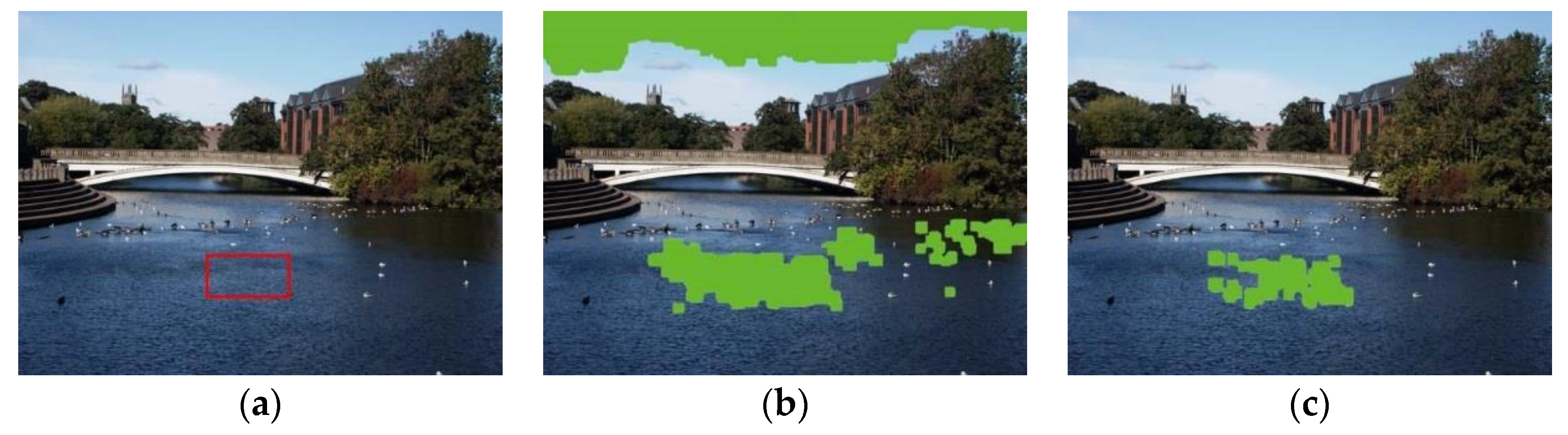
The natural image may have some very similar patches in the background, especially in areas with the same texture, such as sky or lake. They have a high matching degree with their adjacent patches, and are easy to be marked as tampering in the suspicious patches. Such patches are called “false alarm patches”. In order to reduce the false alarm rate of object removal image detection, this paper designs a false alarm removal module based on the analysis of CNN and LSTM network structure. In this module, CNN and LSTM are combined to identify the normal texture consistent area in the image, and then remove the false alarm patches from the suspicious patches, so as to improve the detection accuracy. Figure 3 shows the influence of false alarm patches on the detection results, where Figure 3a is the object removal image with blue sky and water surface background, and the red box indicates the object removal region. In the suspicious patches search, a large number of abnormal similar blocks are detected, including a large number of false alarm patches, as shown in Figure 3b. Obviously, the same texture false alarm regions will interfere with the detection results. Therefore, it is necessary to exclude the false alarm region with consistent texture from the suspicious region. Figure 3c shows the result of filtering suspicious patches by the false alarm elimination module, in which the false alarm caused by the real texture consistent area is removed.
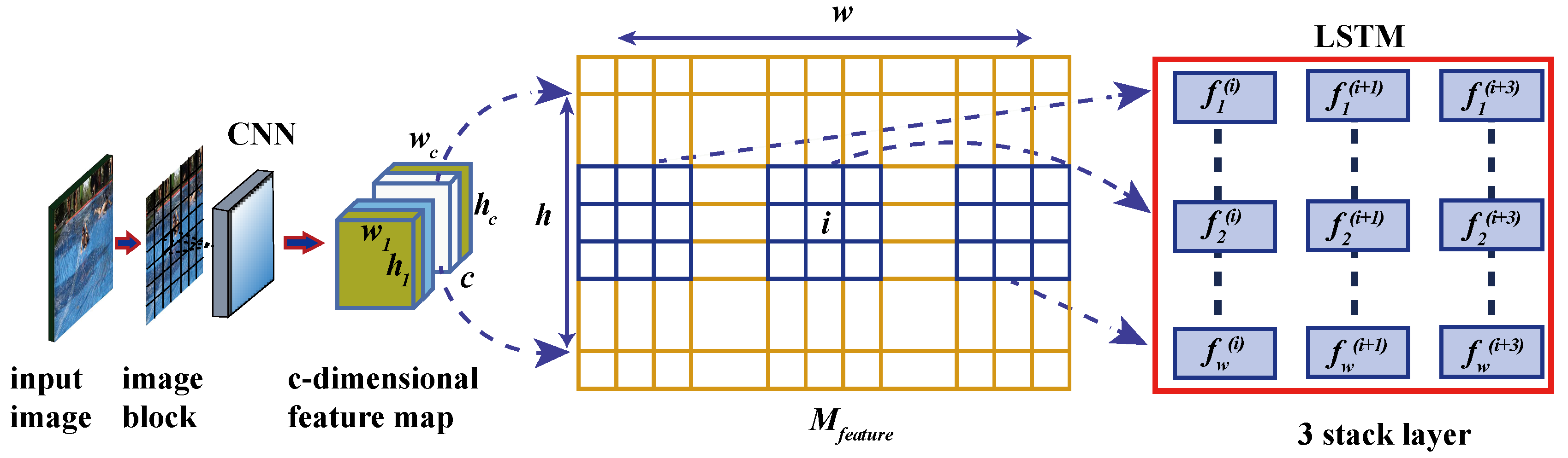
The module consists of a convolution layer [21] and three stacked LSTM stacks. The convolution layer consists of different filters with adaptive weights and biases. The block image is used as the input, and the size is 64 × 64 × 3 (width, height, color channel). The size of the convolution kernel is 3 × 3 × d, where d is the depth of the filter. The filter will create a feature map of the local area connected to the previous layer. The activation function is ReLU [20]. The convolution layer can extract different low-level features from image, which is very important for recognizing false alarm patches. LSTM network is often used to capture the dependency between sequence pixels [22,23]. In this paper, LSTM is used to detect the boundary transformation between different patches in the image, so as to distinguish the normal region and the false alarm region accurately. The specific workflow of the false alarm elimination module is as follows:
Firstly, the image blocks are sent into the convolution layer to generate c feature maps. Each feature map is a feature image Mfeature with the height and width of h and w respectively. Then, a 3 × 3 window is used to slide Mfeature from left to right with step size 1 to obtain h different feature sequences. Then, the filtering vector v is set according to the feature sequence, as shown in Equation (8):
among them, fj(i) ∈ R3 × 3 × c, 1 ≤ j ≤ w, 1 ≤ i ≤ h.
Fi = {(f1(1), f2(1)…, fw(1)), (f1(2), f2(2)…, fw(2)), …, (f1(h), f2(h)…, fw(h))}
Then, the above feature sequences are input into the LSTM network, and each LSTM unit learns the correlation between adjacent patches, by calculating the logarithmic distance between them. The extraction process and LSTM structure of the serialized fj(i) region of each feature map are shown in Figure 4, where i ∈ {1, 2, …, w}, w and h are the width and height of Mfeature respectively, and c is the number of channels. The LSTM network adopts a three-layer stack structure, each layer uses 64 LSTM units, and 64-dimensional feature vectors are obtained from each LSTM unit in the last layer. The feature vectors of all patches are concatenated to form a new c-dimensional feature map. If the feature map of false alarm patches from LSTM is F_LSTM, and the feature map of suspicious patches from CNN is F_CNN, then F_LSTM and F_CNN are isomorphic.
Finally, according to Equation (9), the final feature is selected and projected to the feature map. After decoding, the tamper region location and prediction are represented by the binary mask.
Among them [~] is defined as the selection operation of feature mapping.
F = [F_CNN ~ F_LSTM]
3.3. Filtering of Post-Processing Features
JPEG compression and Gaussian noise are common post-processing operations for tampering images, which are often used by anti-forensics researchers to mask tampering traces. Although the existing methods of image inpainting forensics have achieved some results, the tampered image which has been compressed by JPEG with lower quality factor or added with Gaussian noise with lower signal-to-noise ratio (SNR), or processed by the combination of the above two operations, still cannot be recognized accurately. Aiming at the attacks of the above two post-processing operations, this chapter fully analyzes the influence of post-processing operations on the trace features left by image tampering and the learning characteristics of CNN network itself, and proposes a post-processing feature filtering algorithm. In the detection of tampered images, the CNN network is more focused on learning the trace features introduced by image tampering.
3.3.1. The Filter of JPEG Compression
CNN can extract classification features from data through self-learning, so it is very suitable for the recognition and classification of tampered image trace features [24]. However, JPEG compression belongs to lossy compression, which will inevitably destroy the correlation of discrete cosine transform (DCT) coefficients among pixels and other statistical features. CNN cannot actively select the type of learning features. Generally, CNN tends to learn the features related to image content. Compared with the artificial features introduced by image tampering, they tend to focus on some statistical features, such as the distribution features of the DCT coefficient correlation. In order to make CNN focus more on learning the trace features introduced by image tampering and reduce the impact of post-processing operations. In this paper, a post-processing feature filter module is designed to detect the object removal, based on image inpainting with post-processing operation. The post-processing feature filter module is constrained by the prediction error filter when training the network, to suppress the damage of post-processing operation to the tamper feature.
The module is divided into two layers: the first layer is JPEG compression feature filter layer; the second layer is Gaussian noise filter layer. The post-processing feature filtering module consists of a group of prediction error filters, which are based on the central pixel value of the recommendation window, and the difference between other pixels and the central pixel value is taken as the prediction error. In this way, we need to define learning rules for all k filters in the first layer, as shown in Equation (10):
where ωk (x, y) is the filter weight at (x, y) in the recommended window, and ωk (0, 0) is the filter weight at the center (0, 0) of the recommendation window. Each filter in this layer is initialized by random weight selection, and then the ωk (x, y) weight is reduced according to the learning rules defined in Equation (10). In order to prevent gradient disappearance or gradient explosion, the filter weight is updated by Adam optimization algorithm, and the constraints in Equation (10) are checked again during each iteration. It enables CNN to learn the tampering trace features adaptively, without the influence of JPEG compression. Specifically, the JPEG compression feature filtering algorithm is described as follows:
| Algorithm 1. JPEG compression feature filtering algorithm |
| 1: Input: test image I |
| 2: Output: feature map |
| 3: Initial: the filter weight ωk (k = 1) is randomly selected, and the batch data size is N |
| 4: Begin: |
| 5: The test image I is decomposed into M blocks (i) with size of 32 × 32, where i = 1, 2, …, M; |
| 6: for each block(i) |
| 7: the back-propagation algorithm is used to train the network; |
| 8: ωk is updated with Adam algorithm and back propagation error; |
| 9: the center position (0, 0) of recommended window is determined with ωk; |
| 10: for k <= max_filter_number |
| 11: ωk (0, 0) = 0; |
| 12: ωk (x, y) is updated according to the learning rule as Equation (10); |
| 13: k = k + 1; |
| 14: end for |
| 15 i = i + 1; |
| 16 end for |
| 17: End. |
3.3.2. Gaussian Noise Feature Filtering
Against Gaussian noise attack, this paper fully analyzes the influence of Gaussian noise on the image tampering trace features, and proposes an effective anti-Gaussian noise attack strategy. On this basis, a Gaussian noise feature filter layer is designed to effectively suppress the change of image tampering trace features caused by Gaussian noise features, so as to improve the robustness of the proposed method.
The main idea of Gaussian noise filtering algorithm is to make the loss of local neighborhood caused by Gaussian noise relatively stable. A penalty term needs to be added to the loss function, which is L2 norm of loss gradient. The loss function can be expressed as Equation (11):
where λ is the weight coefficient and E (x, y) is the binary weighted cross entropy, which can be defined as Equation (12):
where z is the output of filter layer, αi, j and βi, j are the weights in x and y directions respectively, and Equation (13) is satisfied:
L (x, y) = E (x, y) + λ ||▽x E (x, y)||2
αi, j + βi, j = 1, αi, j ≥ 0, βi, j ≥ 0
This penalty term makes the loss relatively stable and suppresses the influence of Gaussian noise on CNN feature recognition to the greatest extent. The training process of Gaussian noise filter layer is as follows:
- The training set including image IG-noise and image Iclean is created;
- Assuming that the batch size is N, N images are extracted from the training set each time. The first k images are Gaussian noise images, i.e., {I1G-noise, I2G-noise, …, IKG-noise, IK+1clean, IK+2clean, …, INclean};
- Through the weighted sum of IG-noise image and Iclean image, the losses of batch N images are calculated, which are expressed as Equation (14):where α is the weight parameter, generally 0.2;
- Create a class label for the input image. LGn-true is the real label of IG-noise image, LC-true is the real label of Iclean image, LGn-pre is the prediction label of IG-noise image, LC-pre is the prediction label of Iclean image. In order to make the prediction label closer to the real label, the Adam optimization algorithm is used to update the weight of loss function.
- The gradient direction can be found by calculating the partial derivative of LGn-pre label image. Using the least likelihood class method (LLCM) [25], noise images are classified into the least likelihood class, and the losses of batch N images are minimized in the gradient direction.
In order to ensure that the proposed method can resist different degrees of post-processing attacks, the counter examples of different JPEG quality factors and SNR with uniform distribution are used. No matter whether the input image is post-processing image or not, the model will converge to a relatively small loss point, near which the loss is relatively stable.
4. Network Architecture
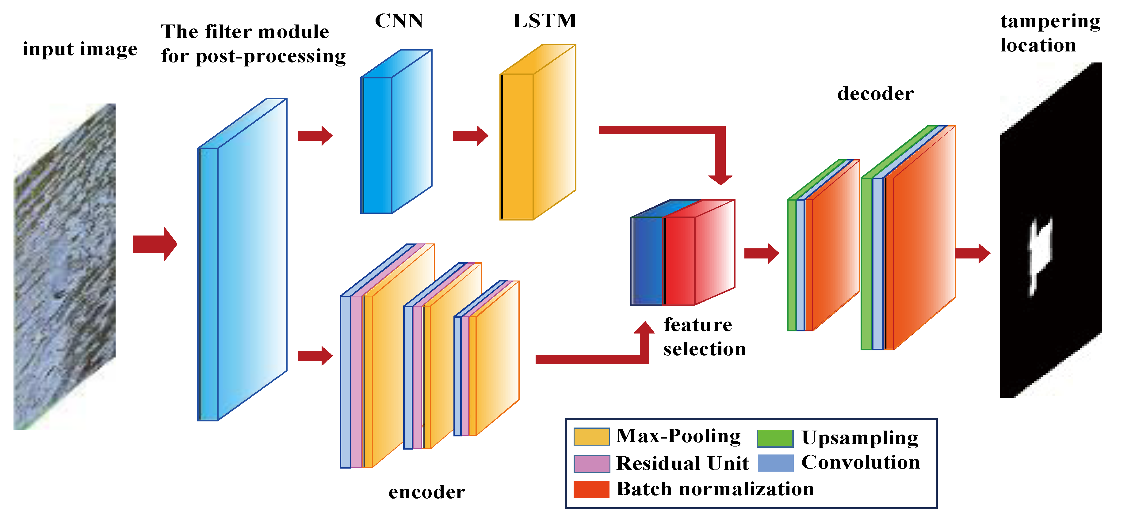
The LSTM-CNN network proposed in this paper is based on the encoder-decoder [26] architecture. The network is divided into three parts: (1) encoder network; (2) decoder network; (3) LSTM network. The encoder and decoder are mainly composed of convolutional neural network (CNN), including convolution layer, residual unit, maximum pooling layer, upper sampling layer and batch normalization layer. Figure 5 shows the overall structure of the LSTM-CNN network, which mainly includes a filter module, two branches and a feature selection module. One branch uses the LSTM network to detect the false alarm patches, the other uses the CNN encoder to search the abnormal similar patches. Finally, the tampered region is located by selecting the feature.
4.1. Encoder Network
In order to effectively identify the abnormal similar region at the pixel level, considering the importance of spatial information to the location of the inpainting region, we exploit the convolution layer to design the encoder, so that the network can identify the abnormal similar region according to the appearance, shape and spatial association between inpainted and uninpainted regions. In the references [27,28,29], some deep structures of image tampering forensics are proposed by using convolution layer. Inspired by this, we designed a new encoder-decoder architecture.
The encoder network consists of different layers of CNN. Each encoder consists of a convolution layer, a residual unit and a pooling layer. The data of each layer are three-dimensional arrays with the size of h × w × c, where h and w are the height and width of image, and c is the dimension of color channel, the size of input image is 256 × 256 × 3 (width, height, color channel).
4.1.1. Convolution Layer
The convolution layer consists of three parts: convolution, activation function and batch normalization, the convolution process follows Equation (15):
where represents the convolution process, Z(∙) is the activation function. The rectifier linear unit (ReLU) [30] is used as the activation function, as shown in Equation (16):
fm,n = max (xm,n, 0)
The convolution layer contains self-learning filters of different sizes. The filters in each layer will create feature maps that connect to the local regions of the previous layer. In each convolution layer, the convolution kernel size is 3 × 3 × d, where d is the filter depth, and different layers in the network use different depths. If the filter depth is too low, it is easy to lead to under fitting, otherwise, it is easy to lead to over fitting if the depth is too high, so it is necessary to select a suitable value. There are three layers in encoder network; the first layer, the second layer and the third layer use 64, 128 and 256 convolution kernels, respectively. In order to prevent the gradient disappearance or gradient explosion caused by data migration in neural network, batch normalization [31] is used in the convolution layer.
4.1.2. Residual Unit
Residual unit is a kind of fast connection without parameters. The main advantage of using residual unit here is that it can easily optimize residual mapping and train more layers. Assuming that the input of the residual element is x and the mapping of the residual element from input to output is M (∙), the output of residual element is M(y) + y.
4.1.3. Pooling Layer
In order to compress the number of image feature parameters and reduce over fitting, a pooling layer [32] is added in the middle of multiple convolution layers to realize feature dimensionality reduction. Pooling method is to use the statistical value of features in the region as the feature value of the region. The common methods are maximum pooling and average pooling. In this paper, the maximum pooling kernel size is 2 × 2 and stride size is 2.
4.2. Decoder Network
The decoder network consists of two layers of the CNN network; each decoder consists of an upper sampling layer, a convolution layer and a batch normalization layer. The upper sampling layer only performs the upper sampling operation on the feature mapping learnt from the previous convolution layer, which does not involve the learnable parameters; the convolution layer uses different multi-channel filters to convolute with the sparse representation of the upper sampling heat map, and then performs the batch normalization operation to generate a denser heat map. Overall, 64 and 16 convolutional kernels of size 3 × 3 are used in the first and second layers of decoder network. Finally, the network outputs a binary mask to represent the tampered region in the image.
In order to compensate for the loss of image spatial resolution caused by the convolution of the encoder, the upper sampling layer is used to enlarge the image. The commonly used upper sampling methods are interpolation, including region interpolation, edge interpolation and bilinear interpolation. In this paper, the bilinear interpolation method [33] is used. In fact, this method makes a linear transformation on the x-axis and y-axis, respectively. The bilinear interpolation method has a large amount of computation, but the image quality is high after processing, and the pixel value will not be discontinuous. The bilinear interpolation up sampling method is used in the two upper sampling layers of decoder network.
4.3. LSTM Network
LSTM is a new type of recurrent neural network (RNN). RNN often encounters the problem of gradient disappearance. LSTM can solve this problem by introducing storage units to determine when to forget some information [34]. LSTM network consists of input layer, hidden layer and output layer. Its main characteristics are the storage unit and three multiplication units in the hidden layer, i.e., input gate, output gate and forgetting gate. The multiplication unit provides read, write and reset operations to the storage unit. The input gate determines the transmission of new information, the output gate determines the output of the current hidden state, and the forgetting gate determines whether to retain the previous information. In this paper, the three gate structures of the LSTM unit adopted by LSTM-CNN are defined as follows (in the following Equation, W represents the weight, b represents the offset term, v represents the filter vector, and σ represents the sigmoid activation function):
- (1)
- Input gate is defined as Equation (17):It = σ (xt W xi + ht−1 W hi + v W vi + yt−1 W yi)
- (2)
- Output gate is defined as Equation (18):Ot = σ (xt W xo + ht−1 W ho + v W vo + yt−1 W yo)
- (3)
- Forget gate is defined as Equation (19):each gate has a value from 0 to 1, which is activated by σ function, and the candidate update unit state (Ct) ~, generated by each LSTM unit, is activated by tanh function, then (Ct) ~ can be expressed as Equation (20):Ft = σ (xt W xf + ht−1 W hf + v W vf + yt−1 W yf)(Ct) ~ = tanh (xt W xc + ht−1 W hc + v W vc + yt−1 W yc)
If the LSTM unit state at the current time t is expressed as Ct, and the output state is expressed as ht, the final unit state Ct can be determined by the unit state Ct−1 at the previous time t − 1 and the candidate update unit state(Ct) ~, and the specific update rules meet the Equation (21):
where ° represents point by point multiplication.
Ct =Ct−1 ° Ft + (Ct) ~ ° It
At the current time t, the hidden output state ht of the LSTM unit can be expressed as Equation (22):
ht = tanh (Ct) ° It
In this paper, xt is the index of patches to be detected, ht is the previous hidden state, v is the filter vector, and yt is the last output false alarm patch index, which can be calculated according to Equation (23):
yt = σ (ht Wyi + b)
5. Experimental Results and Analysis
It is verified that the performance of the proposed LSTM-CNN network for image inpainting forensics through a series of experiments. The hardware environment used in the experiment is Intel® core (TM) i5 7300hq CPU @ 2.5 GHz, memory 8 GB, personal computer with NVIDIA GTX 1050 4G RAM GPU, and software environment is Anaconda Python 3 development tool under Windows 7 system.
5.1. Experimental Setup
The LSTM-CNN network proposed in this paper is based on tensorflow framework [35]. In the process of training, the key step is to select the appropriate optimization algorithm to obtain the best training effect. The commonly used optimization algorithms are stochastic gradient descent (SGD), root mean square propagation (RMSProp) and adaptive moment estimation (Adam). Adam algorithm [36] is selected here. This algorithm combines SGD and RMSProp, and introduces momentum to accelerate the descent in the right direction and suppress the oscillation. At the same time, it avoids the disadvantage of single learning rate.
Because deep learning needs a lot of data to train the network, it usually needs tens of thousands of normal images and tampered images. In order to meet this condition, MIT place2 data set [37] is selected as the training set of data samples in the experiment, which contains 10 million images and more than 400 different types of scene environments. It can be used for visual cognitive tasks with scenes and environments as application contents. We randomly selected 2 × 10⁴ color images, with the size of 256 × 256 as the original image training set.
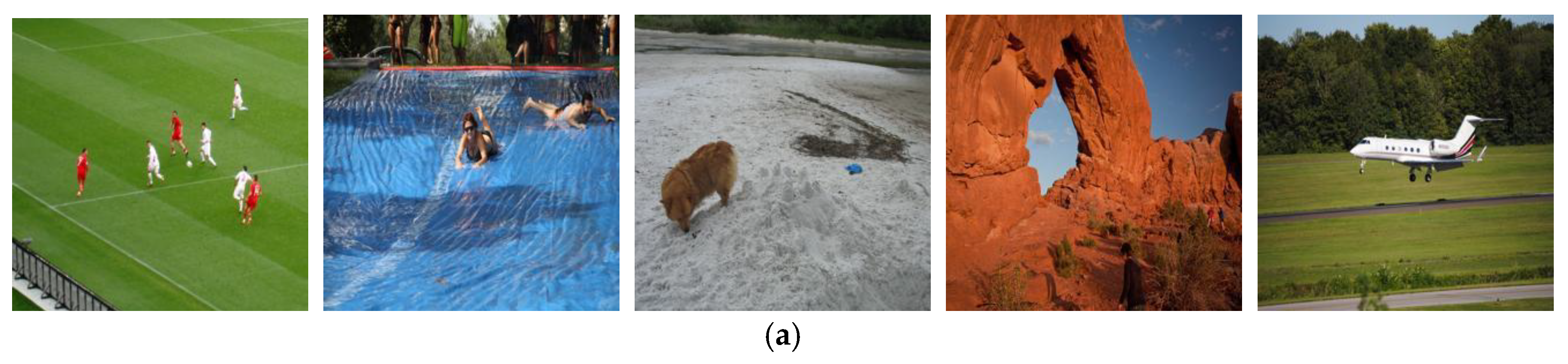
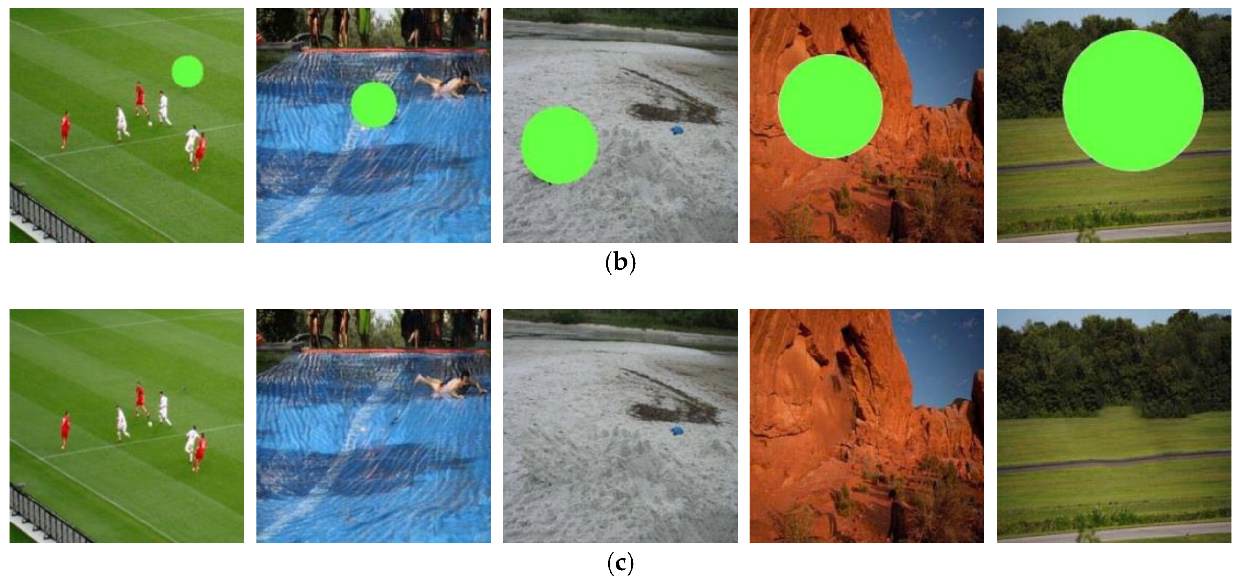
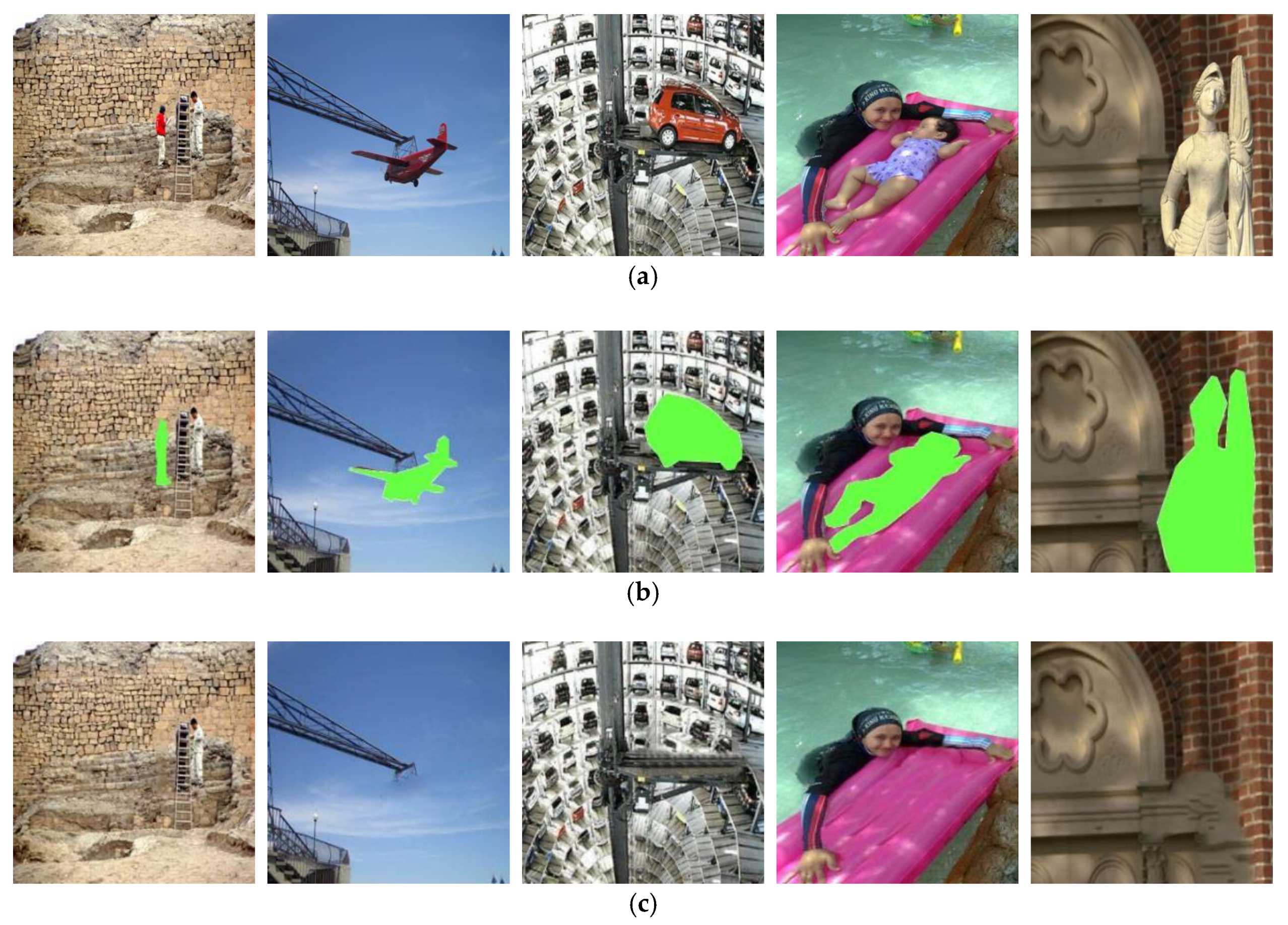
Since there is no public image database for image inpainting forensics, all the tampered images used in the experiment are created by Criminisi’s algorithm. 1 × 10⁴ images are extracted from the original training set, and then tampered by using Criminisi’s algorithm to form tampered regions with different sizes and shapes. In order to facilitate the experimental comparison, the five kinds of images with tampering ratios of 2%, 5%, 10%, 20% and 30% are created respectively. The tampered region is circular or rectangular in shape, and the tampered position is determined by removing a certain object. At the same time, the image with tampered region irregular in shape is generated by the same method, the tampering ratios are 0–5%, 5–10%, 10–20%, 20–30% and 30–40%, respectively. Figure 6 and Figure 7 show the samples of training images with tampered region that are regular and irregular in shape.
In order to fully verify the generality of proposed method for different types of image files and facilitate comparison with other methods, the test samples required for the experiment are taken from uncompressed color image database (UCID) [38], which is widely used in the image forensics. This is because there are only 1338 images in UCID, which cannot meet the needs of deep learning network for the number of data test samples. We enhanced the data of test samples, and took each UCID image as the reference point, which is the upper left point, the upper right point, the lower left point, the lower right point and the center point, and cut the image into the size of 256 × 256. Such an image corresponds to five cropped images, and the number of test image samples can reach 6690. Half of the images in the test set are made in the same way as the tampered images training set, tampered by Criminisi’s algorithm, while the remaining images are retained as normal test images.
In order to verify the robustness of the proposed method to the post-processing, the experiment will verify the performance of method from the following three aspects: (1) the detection for image object removal without post-processing; (2) the detection for image object removal with single post-processing; (3) the detection for image object removal with combined post-processing. In order to make the proposed method comparable, two representative methods are selected, the methods in preference [7] and preference [8], and the accuracy is compared in the same hardware and software environment.
5.2. The Detection for Image Object Removal Without Post-Processing
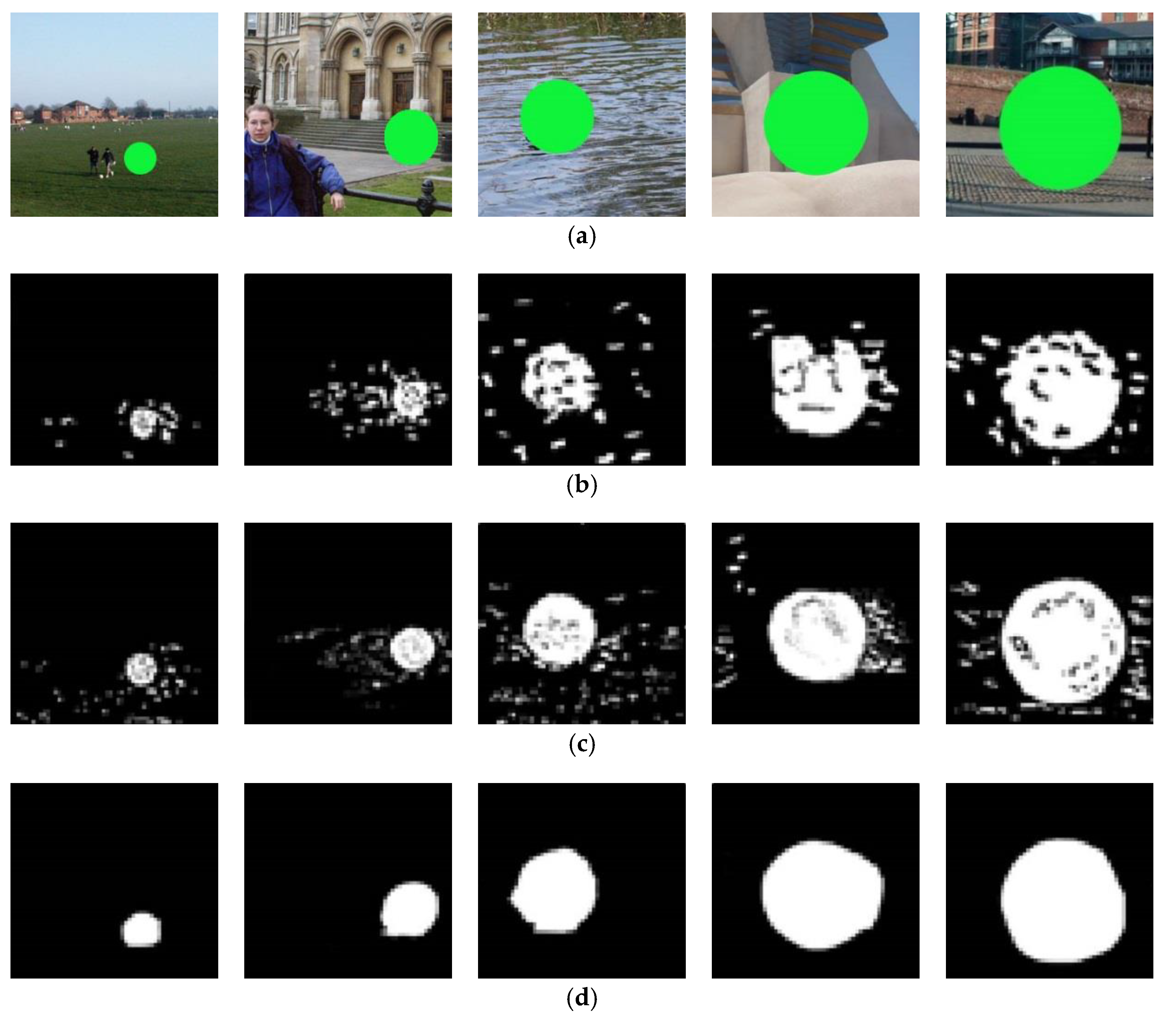
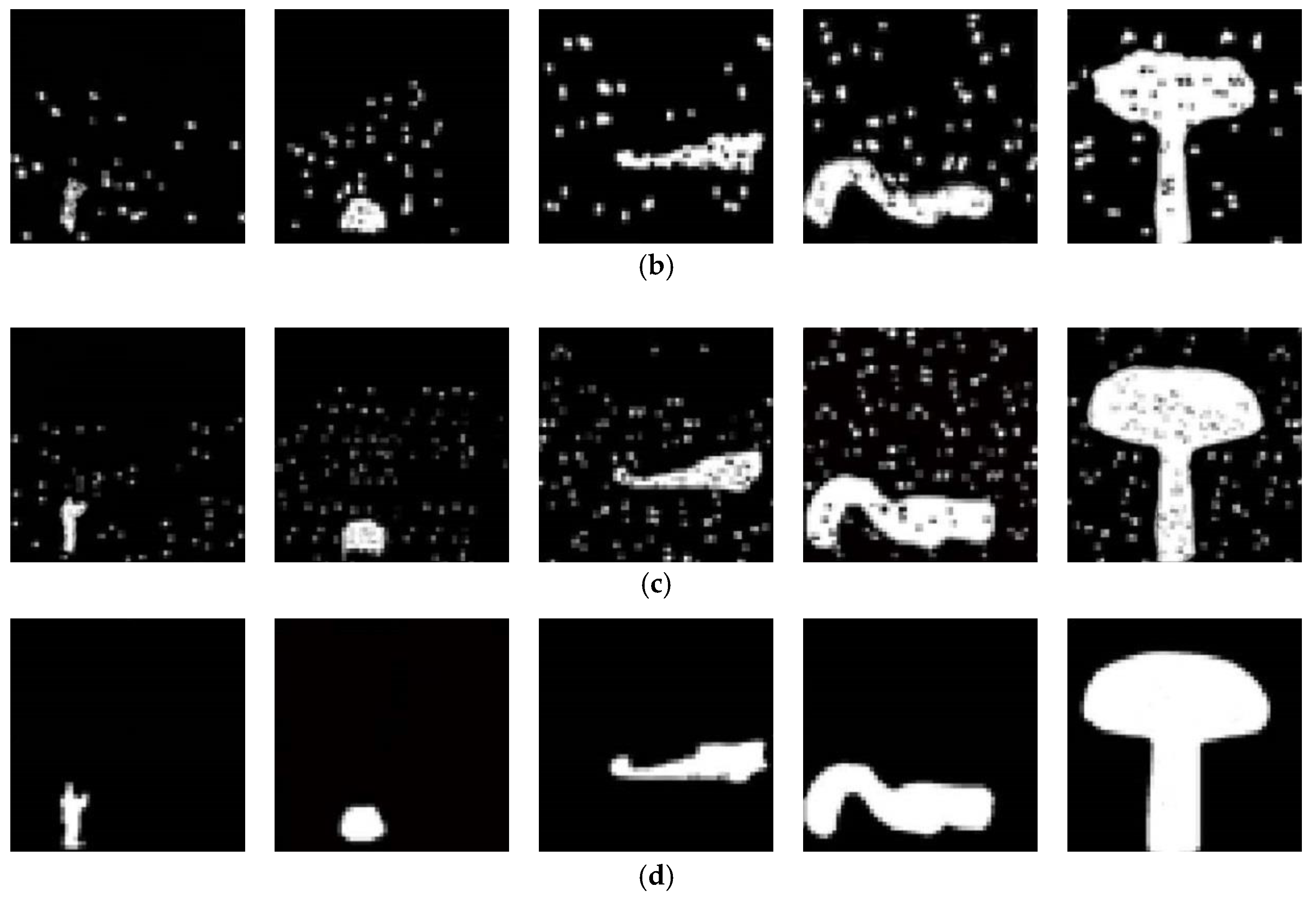
In order to verify the effectiveness of the proposed method, the experiment is divided into two stages: the detection of images with tampered region regular in shape and the detection of images with tampered region irregular in shape. It can be seen from Figure 8 and Figure 9 that, with the increase of the tampering ratio, the identify ability of the three methods for tampered region is enhanced, whether the tampered region is regular or not. However, no matter the size of tampered region, compared with the other two methods, the proposed method can identify tampered region more accurately in position and shape, and get a more consistent detection result with the real tampered region.
As shown in Figure 8d and Figure 9d, due to the similar texture and color distribution in the texture consistent region, it is easy to introduce false alarm pixels, which leads to the increase of false alarm rate. The other two methods output false alarm pixels in different degrees, but the proposed method almost does not output any false alarm pixels.
Table 1 and Table 2 show the accuracy comparison of three methods. The detection accuracy of three methods increase with the tampering ratio, whether the tampering region is regular or not in shape. It is because with the increase of tampering ratio, the abnormal similarity between patches in the image is more obvious, and the boundary between the tampered region and adjacent region is also more obvious. For image detection with low tampering ratio, because the correlation between the tampered region and its adjacent region pixels is not obvious, it is more vulnerable to the influence of false alarm area, resulting in the accuracy of methods to detect image tampering based on this correlation between pixels being low. The proposed method uses the LSTM network to exclude the false alarm region, so it can obtain higher detection accuracy. For the detection of tampered region regular in shape, the performance of the proposed method is slightly poor, and is similar to that of other two methods; for the detection of the tampered region irregular in shape, the difference is obvious. It is mainly that CNN is driven to learn to the regular shape features of tampered region, resulting in a certain over fitting phenomenon. In a word, for all types of tampered regions to be detected, the accuracy of the proposed method is obviously better than other two methods. When the tampering ratio is more than 30%, the accuracy can reach 97.89%. Finally, the mixed tampering ratio (MIX) is tested, the accuracy of proposed method is higher than the other two methods.
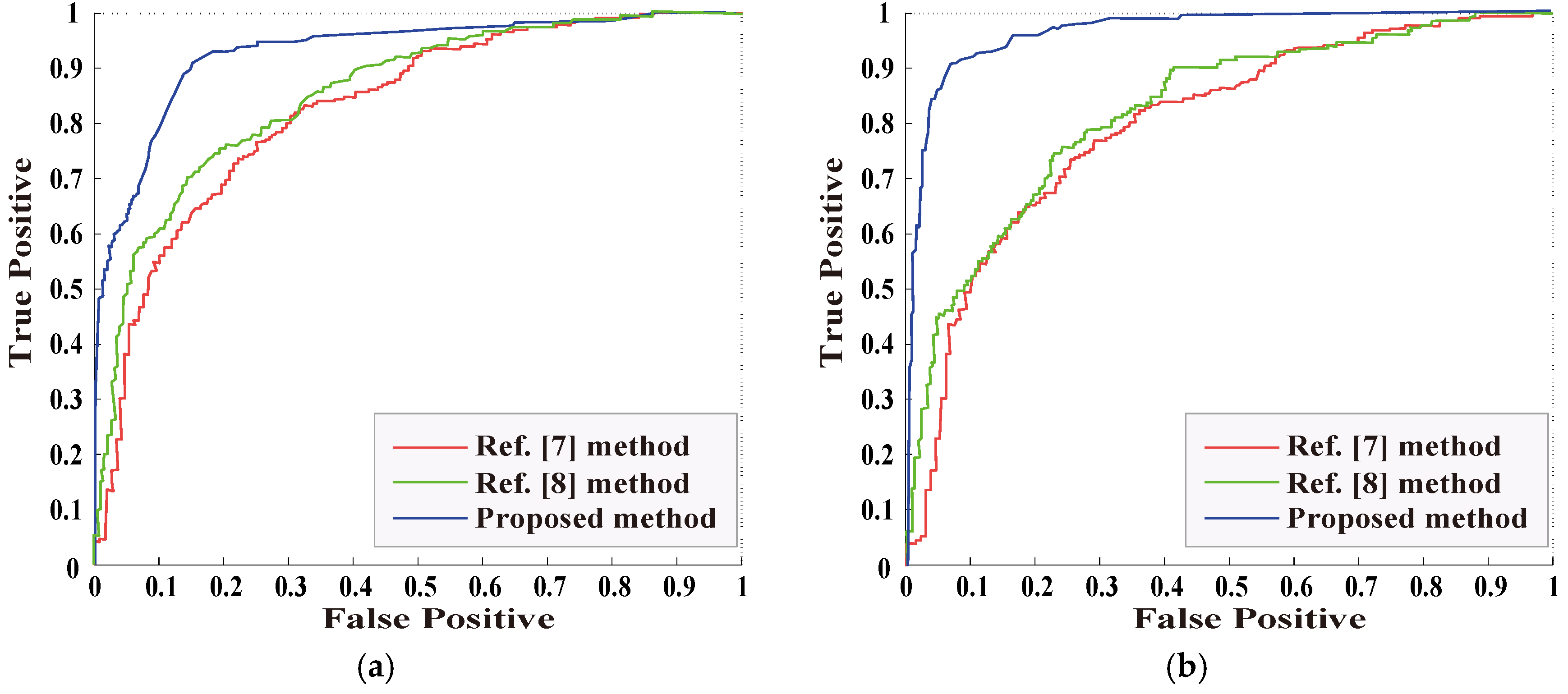
In the experiment, receiver operating characteristic (ROC) curve is used to evaluate the performance of LSTM-CNN model. By selecting the threshold of ROC curve as the point where the sensitivity (true positive rate) and the specificity (true negative rate) are equal, this is the best state of the model performance. Figure 10 shows the ROC curve comparison of the three methods in the case of the mixed test (i.e., the tamper ratio is MIX), where Figure 10a shows the ROC curve when detecting the tampered region regular in shape, and Figure 10b shows the ROC curve when detecting the tampered region irregular in shape. Obviously, the proposed method has a higher AUC value, higher sensitivity and lower false alarm rate.
5.3. The Detection for Image Object Removal with Single Post-Processing
In order to further verify the robustness of the proposed method, the robustness experiment is essential. The post-processing operations include JPEG compression, Gaussian noise, and so on. First of all, we study the object removal detection with single post-processing, then we discuss the detection of post-processing combined operations. The so-called post-processing combined operations refer to the comprehensive application of the above-mentioned post-processing.
5.3.1. The Detection for Object Removal with JPEG Compression
JPEG compression is often used in image post-processing. In this experiment, the images in the test set are compressed into the JPEG image, and their quality factors (QF) are 65%, 70%, 80%, 90% and 95%, respectively. In the experiment, for all the normal images and tampered images in the test set, the tampering ratios and the shape of tampered region are not distinguished, and all of them are mixed together for the test. Table 3 lists the accuracy of the three methods for object removal detection, with JPEG compressed. It can be seen from Table 3 that compared with the other two methods, the proposed method has the highest detection accuracy. When the image quality factor is low, such as QF = 65, the detection accuracy of the methods in [7,8] is obviously low, and the detection results are not ideal. The two methods do not fully consider the impact of JPEG compression on the forensics clues of image inpainting. JPEG compression will change the correlation between DCT coefficients of the image, which is not conducive to those image tampering detection methods that seek the correlation between the tamper region and its neighborhood DCT coefficients as forensics clues. The proposed method restrains CNN’s learning about JPEG compression features, and makes it more focused on learning the trace features of image tampering, thus avoiding this problem.
5.3.2. The Detection for Object Removal with Gaussian Noise
In order to cover up the image tampering trace, adding Gaussian noise to a tampered image is also a kind of image post-processing operation commonly used by tampers. It is also necessary to carry out the robustness experiment for the post-processing of Gaussian noise. For all images in the test set, Gaussian noise with signal noise ratio (SNR) of 25 dB, 30 dB, 35 dB, 40 dB and 45 dB is added. Table 4 shows the detection accuracy of the three methods under Gaussian noise. From the data in the table, it can be clearly found that when SNR is low, such as SNR = 25 dB, the accuracy of the methods in preference [7] and preference [8] are very low, but the proposed method can obtain high accuracy. It is because the correlation of adjacent pixels has changed due to the addition of Gaussian noise. In this paper, by adjusting the filter, the feature loss caused by Gaussian noise is minimized, thus improving the detection accuracy.
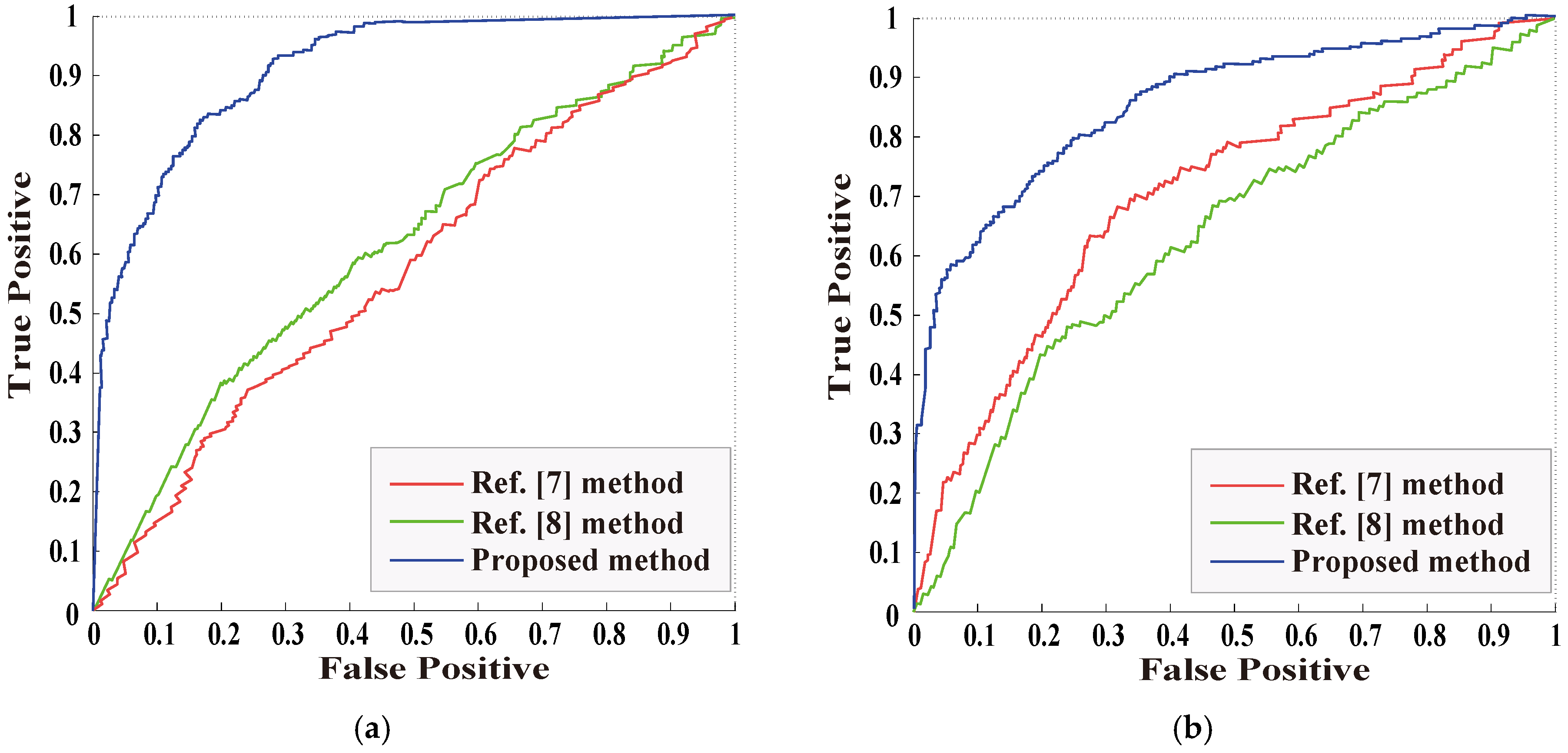
For the object removal detection performance with JPEG compression and Gaussian noise, ROC curve is used to evaluate the experiment. Figure 11 shows the ROC curve comparison of the three methods. Figure 11a shows the ROC curve of the object removal image detection with JPEG compression, and Figure 11b shows the ROC curve of the object removal image detection with Gaussian noise. As can be seen from Figure 11, the proposed method has superior performance and strong robustness to JPEG compression and Gaussian noise post-processing.
5.4. The Detection for Image Object Removal with Combined Post-Processing
In order to eliminate the trace features left by image tampering to a great extent, the researchers of anti-forensics technology not only use a kind of post-processing operation, but also use a variety of post-processing combined operations, which makes the detection performance of forensics technology greatly reduced or invalid. Therefore, it is necessary to carry out the robustness experiment for tampered image detection with combined post-processing. The experiment mainly verifies the performance of the proposed method to resist the combined attack of JPEG compression and Gaussian noise. In order to fully study the influence of JPEG compression and Gaussian noise on forensics performance, data samples are prepared in the following way: JPEG compression and Gaussian noise are performed on all images in the test set respectively, and the quality factor and SNR are taken from the extreme cases of the above experimental data samples, namely QF = 65 and QF = 95, SNR = 25 dB and SNR = 45 dB, and then four groups of data samples are obtained through combination. The accuracy of the three methods for object removal detection with combined post-processing operation is shown in Table 5. When the quality factor and SNR are both low, the accuracy of the proposed method is much higher than other two methods, which shows that the proposed methods have a strong ability to resist the combined post-processing operation attack; when the quality factor and SNR are both high, the accuracy of the proposed method is slightly higher than the other two methods, which shows that the advantages of the proposed method are not fully played. When quality factor is high and SNR is low, the accuracy of the method in reference [7] is slightly higher than that in reference [8]; when quality factor is low and SNR is high, the accuracy of the method in reference [8] is slightly higher than that in reference [7]. Although the proposed method is superior to the other two methods in both cases, the performance is better in the case of low-quality factor and high SNR.
It is mainly because the methods in reference [7,8] use slightly different forensics features, and the influence of JPEG compression and Gaussian noise on forensics is different. The proposed method is to identify the occurrence of object removal by pixel level, so it is more affected by Gaussian noise, but the overall detection performance is better than the other two methods.
6. Conclusions
In this paper, an object removal detection method of exemplar-based image inpainting is proposed. Aimed at the shortcomings of existing image inpainting forensics methods, such as time-consuming for similar patches search, high false alarm rate and poor robustness of post-processing, a new encoder-decoder network is constructed by combining CNN and LSTM to detect the image inpainting with single and combined post-processing operations. First, CNN identifies suspicious similar patches in tampered images. Different from other supervised learning methods, which need to input pairs of patches to calculate the similarity between patches, the proposed method can learn the similarity between pixels point by point, so it is suitable for large-scale data sets. Then, the LSTM network is used to identify the normal texture consistent regions from suspicious area. Finally, the interference of post-processing operation on image inpainting detection is eliminated by the filtering module. A large number of experiments verify the effectiveness of this method; compared with the existing representative methods, the accuracy of proposed method is higher, and the prediction performance of the model is greatly improved.
Author Contributions
Conceptualization, M.L. and S.N.; methodology, M.L.; software, M.L.; validation, M.L. and S.N.; formal analysis, M.L.; investigation, M.L.; writing—original draft preparation, M.L.; writing—review and editing, M.L.; visualization, M.L.; supervision, S.N.; project administration, S.N.; funding acquisition, S.N. All authors have read and agreed to the published version of the manuscript.
Funding
The authors received no specific funding for this study.
Conflicts of Interest
The authors declare no conflict of interest.
References
- Criminisi, A.; Prez, P.; Toyama, K. Region filling and object removal by exemplar based image inpainting. IEEE Trans. Image Process. 2004, 13, 1200–1212. [Google Scholar] [CrossRef]
- Awati, P. Digital image inpainting based on median diffusion and directional median filtering. Int. J. Comput. Appl. 2014, 3, 35–39. [Google Scholar]
- Guillemot, C.; Meur, O.L. Image inpainting: Overview and recent advances. IEEE Signal Process. Mag. 2014, 31, 127–144. [Google Scholar] [CrossRef]
- Bertalmio, M.; Sapiro, G.; Caselles, V.; Balleste, C. Image Inpainting. In Proceedings of the International Conference on Computer Graphics and Interactive Techniques, New York, NY, USA, 10–13 July 2000; pp. 417–424. [Google Scholar]
- Wu, Q.; Sun, S.; Zhu, W.; Li, G.H.; Tu, D. Detection of digital doctoring in exemplar-based inpainted Images. In Proceedings of the IEEE International Conference on Machine Learning and Cybernetics, Kunming, China, 12–15 July 2008; IEEE: Los Alamitos, CA, USA, 2008; pp. 1222–1226. [Google Scholar]
- Bacchuwar, K.; Ramakrishnan, K. A jump patch-block match algorithm for multiple forgery detection. In Proceedings of the IEEE International Multi-Conference on Automation, Computing, Communication, Control and Compressed Sensing, Kottayam, India, 12–14 June 2013; pp. 723–728. [Google Scholar]
- Chang, I.; Yu, J.; Chang, C. A forgery detection algorithm for exemplar-based inpainting images using multi-region relation. Image Vis. Comput. 2013, 31, 57–71. [Google Scholar] [CrossRef]
- Liang, Z.; Yang, G.; Ding, X.; Li, L. An efficient forgery detection algorithm for object removal by exemplar-based image inpainting. J. Vis. Commun. Image Represent. 2015, 30, 75–85. [Google Scholar] [CrossRef]
- Zhao, Y.; Liao, M.; Shih, F.; Shi, Y. Tampered region detection of inpainting JPEG images. Opt. Int. J. Light Electron Opt. 2013, 124, 2487–2492. [Google Scholar] [CrossRef]
- Liu, Q.; Zhou, B.; Sung, A.; Qiao, M. Exposing in painting forgery in JPEG images under recompression attacks. In Proceedings of the IEEE International Conference on Machine Learning and Applications, Anaheim, CA, USA, 18–20 December 2016; pp. 164–169. [Google Scholar]
- Zhang, D.; Liang, Z.; Yang, G.; Li, Q.; Li, L.; Sun, X. A robust forgery detection algorithm for object removal by exemplar-based image inpainting. Multimed. Tools Appl. 2018, 77, 11823–11842. [Google Scholar] [CrossRef]
- Jung, M.; Bresson, X.; Chan, T. Nonlocal Mumford–Shah regularizers for color image restoration. IEEE Trans. Image Process. 2011, 20, 1583–1598. [Google Scholar] [CrossRef] [PubMed] [Green Version]
- Shen, J.; Chan, T.F. Mathematic models for local non-Texture inpainting. Siam J. Appl. Math. 2001, 62, 1019–1043. [Google Scholar] [CrossRef]
- Xu, L.; W, Y.; Zhang, B. Image inpainting algorithm based on adaptive high order variation in eight neighbors. J. Graph. 2017, 38, 129–138. [Google Scholar]
- Chan, T.F.; Shen, J. Nontexture inpainting by curvature-driven diffusions. J. Vis. Commun. Image Represent. 2001, 12, 436–449. [Google Scholar] [CrossRef]
- Liu, Y.; Caselles, V. Exemplar-based image inpainting using multiscale graph cuts. IEEE Trans. Image Process. 2013, 22, 1699–1711. [Google Scholar] [PubMed]
- Jing, W.; Ke, L.; Pan, D.; He, B.; Bing, K.B. Robust object removal with an exemplar-based image inpainting approach. Neurocomputing 2014, 123, 150–155. [Google Scholar]
- Barnes, C.; Hechtman, E.; Goldman, D.; Finkelstein, A. The generalized patch match correspondence algorithm. Eur. Conf. Comput. Vis. 2010, 6313, 29–43. [Google Scholar]
- Sun, T.; Sun, L.; Yeung, D. Fine-grained categorization via CNN-based automatic extraction and integration of object-level and part-level features. Image Vis. Comput. 2017, 64, 47–66. [Google Scholar] [CrossRef]
- Kamaledin, G. Generalizing the convolution operator in convolutional neural networks. Neural Process. Lett. 2019, 2, 1–15. [Google Scholar]
- Hsieh, T.; Su, L.; Yang, Y.H. A Streamlined Encoder/decoder Architecture for Melody Extraction. In Proceedings of the 2019 IEEE International Conference on Acoustics, Speech and Signal Processing (ICASSP), Brighton, UK, 12–17 May 2019. [Google Scholar]
- Saman, S. French Word Recognition through a Quick Survey on Recurrent Neural Networks Using Long-Short Term Memory RNN-LSTM. Am. Sci. Res. J. Eng. Technol. Sci. 2018, 39, 250–267. [Google Scholar]
- Pinheiro, P.; Collobert, R. Recurrent convolutional neural networks for scene labeling. In Proceedings of the International Conference on Machine Learning, Beijing, China, 21–26 June 2014. [Google Scholar]
- Bondi, L.; Lameri, S.; Guera, D.; Bestagini, P.; Delp, E.J.; Tubar, S. Tampering detection and localization through clustering of camera-based cnn features. In Proceedings of the The IEEE Conference on Computer Vision and Pattern Recognition Workshops, Honolulu, HI, USA, 21–26 July 2017; pp. 1855–1864. [Google Scholar]
- Ishikawa, S.; Zhukova, A.; Iwasaki, W.; Gascuel, O. A Fast Likelihood Method to Reconstruct and Visualize Ancestral Scenarios. Mol. Biol. Evol. 2019, 9, 2069–2085. [Google Scholar] [CrossRef] [Green Version]
- Kendall, A.; Badrinarayanan, V.; Cipolla, R. Bayesian segnet: Model uncertainty in deep convolutional encoder-decoder architectures for scene understanding. Comput. Sci. 2015, 15, 1511–1613. [Google Scholar]
- Shi, Z.; Shen, X.; Kang, H.; Lv, Y. Image Manipulation Detection and Localization Based on the Dual-Domain Convolutional Neural Networks. IEEE Access 2018, 6, 76437–76453. [Google Scholar] [CrossRef]
- Chen, Y.; Kang, X.; Shi, Y.Q.; Wang, Z.J. A multi-purpose image forensic method using densely connected convolutional neural networks. J. Real Time Image Process. 2019, 16, 725–740. [Google Scholar] [CrossRef]
- Bondi, L.; Baroffio, L.; Güuera, D.; Bestagini, P.; Delp, E.J.; Tubaro, S. First Steps Toward Camera Model Identification with Convolutional Neural Networks. IEEE Signal Process. Lett. 2016, 24, 259–263. [Google Scholar] [CrossRef] [Green Version]
- Shan, C.; Guo, X.; Ou, J. Deep leaky single-peaked triangle neural networks. Int. J. Control Autom. Syst. 2019, 17, 5786. [Google Scholar] [CrossRef]
- Dong, N.; Li, W.; Adeli, E.; Lao, C.; Lin, W.; Shen, D. 3-d fully convolutional networks for multimodal isointense infant brain image segmentation. IEEE Trans. Cybern. 2019, 49, 1123–1136. [Google Scholar]
- Wang, Y.; Li, M.; Pan, Z.; Zheng, J. Pulsar candidate classification with deep convolutional neural networks. Res. Astron. Astrophys. 2019, 19, 133. [Google Scholar] [CrossRef] [Green Version]
- Hu, J.; Chen, Z.; Yang, M.; Zhang, R.; Cui, W. A multi-scale fusion convolutional neural network for plant leaf recognition. IEEE Signal Process. Lett. 2018, 25, 853–857. [Google Scholar] [CrossRef]
- Nguyen, V.-H.; Nguyen, M.-T.; Choi, J.; Kim, Y.-H. NLOS Identification in WLANs Using Deep LSTM with CNN Features. Sensors 2018, 18, 4057. [Google Scholar] [CrossRef] [Green Version]
- Chollet, F.; Keras, F. Deep Learning Library for Theano and Tensorflow. Available online: https://github.com/fchollet/keras (accessed on 6 November 2019).
- Yang, G.; Yang, J.; Li, S.; Hu, J. Modified cnn algorithm based on dropout and adam optimizer. J. Huazhong Univ. Sci. Technol. (Nat. Sci. Ed.) 2018, 46, 122–127. [Google Scholar]
- Zhou, B.; Lapedriza, A.; Xiao, J.; Torralba, A.; Oliva, A. Learning deep features for scene recognition using places database. Adv. Neural Inf. Process. Syst. 2014, 27, 487–495. [Google Scholar]
- Schaefer, G.; Stich, M. UCID-an uncompressed color image database. Storage Retr. Methods Appl. Multimed. 2004, 5307, 472–480. [Google Scholar]
Figure 1.
An example of object removal using image inpainting: (a) original image; (b) inpainted image.
Figure 1.
An example of object removal using image inpainting: (a) original image; (b) inpainted image.

Figure 2.
Schematic diagram of criminisi’s algorithm: (a) region Ω to be inpainted; (b) selecting patch Ψp to be inpainted; (c) searching the best matching patch Ψq`; (d) inpainting the patch Ψp with Ψq`.
Figure 2.
Schematic diagram of criminisi’s algorithm: (a) region Ω to be inpainted; (b) selecting patch Ψp to be inpainted; (c) searching the best matching patch Ψq`; (d) inpainting the patch Ψp with Ψq`.

Figure 3.
The effect of false alarm patches on object removal detection: (a) the image with object removed; (b) the search effect of suspicious block; (c) the effect of removing false alarm block.
Figure 3.
The effect of false alarm patches on object removal detection: (a) the image with object removed; (b) the search effect of suspicious block; (c) the effect of removing false alarm block.

Figure 4.
Serialization process of long short-term memory (LSTM) network feature mapping.

Figure 5.
LSTM-convolutional neural network (CNN) network structure.

Figure 6.
The sample of training images with tampered region regular in shape: (a) the sample of original image in training set; (b) tampered region marked by green mask; (c) the sample of tampered image generated from training set.
Figure 6.
The sample of training images with tampered region regular in shape: (a) the sample of original image in training set; (b) tampered region marked by green mask; (c) the sample of tampered image generated from training set.


Figure 7.
The sample of training images with tampered region regular in shape: (a) the sample of original image in training set; (b) tampered region marked by green mask; (c) the sample of tampered image generated from training set.
Figure 7.
The sample of training images with tampered region regular in shape: (a) the sample of original image in training set; (b) tampered region marked by green mask; (c) the sample of tampered image generated from training set.

Figure 8.
The detection results of tampered region regular in shape: (a) the sample images with the tampered region (the tampering ratio: 2%, 5%, 10%, 20% and 30%); (b) the detection results of preference [7] method; (c) the detection results of preference [8] method; (d) the detection results of proposed method.

Figure 9.
The detection results of tampered region irregular in shape: (a) the sample images with the tampered region (the tampering ratio: 0–5%, 5–10%, 10–20%, 20–30% and 30–40%); (b) the detection results of preference [7] method; (c) the detection results of preference [8] method; (d) the detection results of the proposed method.


Figure 10.
Receiver operating characteristic (ROC) curve of object removal image detection without post-processing: (a) the detection of tampered region regular in shape; (b) the detection of tampered region regular in shape.
Figure 10.
Receiver operating characteristic (ROC) curve of object removal image detection without post-processing: (a) the detection of tampered region regular in shape; (b) the detection of tampered region regular in shape.

Figure 11.
ROC curve of object removal image detection without post-processing: (a) the detection of tampered region regular in shape; (b) the detection of tampered region regular in shape.
Figure 11.
ROC curve of object removal image detection without post-processing: (a) the detection of tampered region regular in shape; (b) the detection of tampered region regular in shape.


Table 1.
The comparison of detection accuracy (tampered region regular in shape).
| Tampering Ratio (%) | Ref. [7] Method (%) | Ref. [8] Method (%) | Proposed Method (%) |
|---|---|---|---|
| 2 | 80.65 | 82.87 | 84.28 |
| 5 | 84.36 | 86.98 | 88.46 |
| 10 | 87.62 | 88.91 | 93.64 |
| 20 | 91.28 | 92.66 | 95.45 |
| 30 | 95.31 | 96.56 | 96.78 |
| MIX | 90.35 | 91.58 | 93.87 |
Table 2.
The comparison of detection accuracy (tampered region irregular in shape).
| Tampering Ratio (%) | Ref. [7] Method (%) | Ref. [8] Method (%) | Proposed Method (%) |
|---|---|---|---|
| 0–5 | 78.57 | 79.26 | 87.86 |
| 5–10 | 81.65 | 82.98 | 90.36 |
| 10–20 | 84.28 | 86.11 | 94.64 |
| 20–30 | 88.28 | 89.66 | 96.95 |
| 30–40 | 92.31 | 93.56 | 97.89 |
| MIX | 85.59 | 86.88 | 94.87 |
Table 3.
The detection accuracy of object removal image with JPEG compression.
| Quality Factor (%) | Ref. [7] Method (%) | Ref. [8] Method (%) | Proposed Method (%) |
|---|---|---|---|
| 65 | 45.75 | 45.89 | 86.63 |
| 70 | 52.95 | 53.28 | 88.86 |
| 80 | 66.48 | 66.96 | 91.64 |
| 90 | 82.58 | 83.66 | 93.95 |
| 95 | 92.03 | 93.56 | 96.89 |
| MIX | 71.92 | 72.38 | 91.75 |
© 2020 by the authors. Licensee MDPI, Basel, Switzerland. This article is an open access article distributed under the terms and conditions of the Creative Commons Attribution (CC BY) license (http://creativecommons.org/licenses/by/4.0/).
Share and Cite
MDPI and ACS Style
Lu, M.; Niu, S. A Detection Approach Using LSTM-CNN for Object Removal Caused by Exemplar-Based Image Inpainting. Electronics 2020, 9, 858. https://0-doi-org.brum.beds.ac.uk/10.3390/electronics9050858
AMA Style
Lu M, Niu S. A Detection Approach Using LSTM-CNN for Object Removal Caused by Exemplar-Based Image Inpainting. Electronics. 2020; 9(5):858. https://0-doi-org.brum.beds.ac.uk/10.3390/electronics9050858
Chicago/Turabian StyleLu, Ming, and Shaozhang Niu. 2020. "A Detection Approach Using LSTM-CNN for Object Removal Caused by Exemplar-Based Image Inpainting" Electronics 9, no. 5: 858. https://0-doi-org.brum.beds.ac.uk/10.3390/electronics9050858
Note that from the first issue of 2016, this journal uses article numbers instead of page numbers. See further details here.