Towards Efficient Neuromorphic Hardware: Unsupervised Adaptive Neuron Pruning
by
 , , , and
Wenzhe Guo
1 ,
,
Hasan Erdem Yantır
1,
Mohammed E. Fouda
2,
Ahmed M. Eltawil
1,2 and
Khaled Nabil Salama
1,*
1
Division of Computer, Electrical and Mathematical Sciences and Engineering, King Abdullah University of Science and Technology, Thuwal 23955, Saudi Arabia
2
Department of Electrical Engineering and Computer Science, University of California-Irvine, Irvine, CA 92612, USA
*
Author to whom correspondence should be addressed.
Electronics 2020, 9(7), 1059; https://0-doi-org.brum.beds.ac.uk/10.3390/electronics9071059
Submission received: 14 May 2020
/
Revised: 6 June 2020
/
Accepted: 23 June 2020
/
Published: 27 June 2020
(This article belongs to the Special Issue Low-Power Techniques for Embedded Systems and Network-on-Chip Architectures)
Abstract
:To solve real-time challenges, neuromorphic systems generally require deep and complex network structures. Thus, it is crucial to search for effective solutions that can reduce network complexity, improve energy efficiency, and maintain high accuracy. To this end, we propose unsupervised pruning strategies that are focused on pruning neurons while training in spiking neural networks (SNNs) by utilizing network dynamics. The importance of neurons is determined by the fact that neurons that fire more spikes contribute more to network performance. Based on these criteria, we demonstrate that pruning with an adaptive spike count threshold provides a simple and effective approach that can reduce network size significantly and maintain high classification accuracy. The online adaptive pruning shows potential for developing energy-efficient training techniques due to less memory access and less weight-update computation. Furthermore, a parallel digital implementation scheme is proposed to implement spiking neural networks (SNNs) on field programmable gate array (FPGA). Notably, our proposed pruning strategies preserve the dense format of weight matrices, so the implementation architecture remains the same after network compression. The adaptive pruning strategy enables 2.3× reduction in memory size and 2.8× improvement on energy efficiency when 400 neurons are pruned from an 800-neuron network, while the loss of classification accuracy is 1.69%. And the best choice of pruning percentage depends on the trade-off among accuracy, memory, and energy. Therefore, this work offers a promising solution for effective network compression and energy-efficient hardware implementation of neuromorphic systems in real-time applications.
1. Introduction
The human brain is considered as the most complex, energy-efficient, and intelligent control system since it is responsible for supervising the functions of the body, interpreting external information, taking appropriate actions and most importantly, embodies the essence of our mind [1]. These facts lead researchers to embrace brain-inspired computing as a new paradigm to deal with increasingly complex computational problems. In recent years, neuromorphic systems built on spiking neural networks (SNNs) have attracted significant attention due to asynchronous event-driven computation and massively parallel architecture [2,3,4]. To solve real-time challenges, a quest for improving the energy efficiency of SNNs becomes necessary [5].
It is a general belief that neurons and synapses are produced rapidly before two years of age in human brains [6]. Subsequently, a large number of neurons and synapses are pruned away during the individual development process. Specifically, 40% of cortical neurons could be eliminated during childhood [7]. Pruning is a purposeful process that improves the efficiency of information transmission in the brain. Inspired by biological evolution, researchers have applied pruning in artificial neural networks (ANNs) to improve network performance [8]. Pruning removes redundant network parameters and alleviates the over-fitting problem. Furthermore, pruning reduces network size and redundant connections, which brings down memory storage and energy consumption in hardware. Generally, pruning can be carried out in two different ways, which are weight pruning and neuron pruning [9]. Weight pruning removes unimportant synaptic connections by examining their relevance to outputs. In this way, the pruned weight matrices become sparse. However, in general, weight pruning is conducted in an unstructured way without following a specific geometry and constraint to increase the sparsity percentage. In order to leverage the sparsity for memory reduction, the irregular structure of the weight matrices often requires an encoding scheme to store the non-zero weights and extra computational time to decode the sparse format before conducting algebra operations [9]. Thus, the resulting sparsity often causes performance degradation, particularly for highly parallel hardware architectures specialized for fast linear algebra operations on regular data (e.g., matrix multiplications) [9]. To overcome these challenges, neuron pruning was suggested to be a more effective approach. Neuron pruning takes away entire non-relevant neurons, which leads to many benefits—(1) Neuron pruning reduces the network parameters significantly where all the synapses associated with the pruned neuron are pruned as well. Thus, it provides speedup and energy reduction; (2) Neuron pruning eliminates the entire rows/columns in the weight matrices reducing the weight matrices’ dimensions proportionally, which could be efficiently implemented in the hardware compared to unstructured weight pruning [9]; (3) It also provides a way to determine the optimal number of neurons for a given network architecture [10]. Accordingly, many works have proposed various approaches to implement neuron pruning for the pursuit of a balance between compression ratio and accuracy [10,11,12,13,14].
Pruning has been extensively studied in ANNs because of its great success, whereas a very limited amount of works have been done in SNNs [15,16,17,18]. In Reference [15], authors propose pruning neurons by comparing their class-wise dominance with a certain threshold in a supervised way. In Reference [17], a post-training neuron pruning method was used to reduce the network size by comparing the spiking frequency of a neuron with average output spike frequency. In Reference [18], a supervised pruning strategy was demonstrated by evaluating the similarity between neurons and pruning similar neurons. However, these ideas are based on either post-training pruning or supervised pruning. Pruning neurons during unsupervised training in SNNs has yet to be explored. The benefit of online pruning lies in being able to improve training energy efficiency and convergence time. This approach is crucial to developing online learning systems for real-world applications, especially in an unsupervised way.
In this paper, we propose different strategies for pruning neurons during unsupervised training in SNNs and digital implementations to demonstrate significantly reduced memory size and improved energy efficiency. The main contributions of this paper are summarized as follows:
- Three different strategies for pruning neurons are proposed by exploiting network dynamics in unsupervised SNNs. An adaptive neuron online pruning strategy can effectively reduce network size and maintain high classification accuracy.
- The adaptive neuron online pruning strategy outperforms post-training pruning, which shows significant potential for online training by improving both training energy efficiency and classification accuracy.
- A parallel digital implementation scheme is presented. The adaptive neuron pruning strategy enables significant memory size reduction and energy efficiency improvement.
- The proposed pruning strategies preserve the dense structure of the weight matrix. No additional compression technique is required for the implementation of pruned SNNs.
2. Pruning Strategies
In this section, we will introduce SNN architecture and propose three different strategies to prune neurons while training, namely, (1) online constant pruning, (2) online constant-threshold pruning, and (3) online adaptive pruning. During training, the neuron pruning process will be repeated multiple times by dividing a whole dataset into multiple batches. The batch size is selected as 5000 under the consideration of pruning frequency.
2.1. Network Architecture
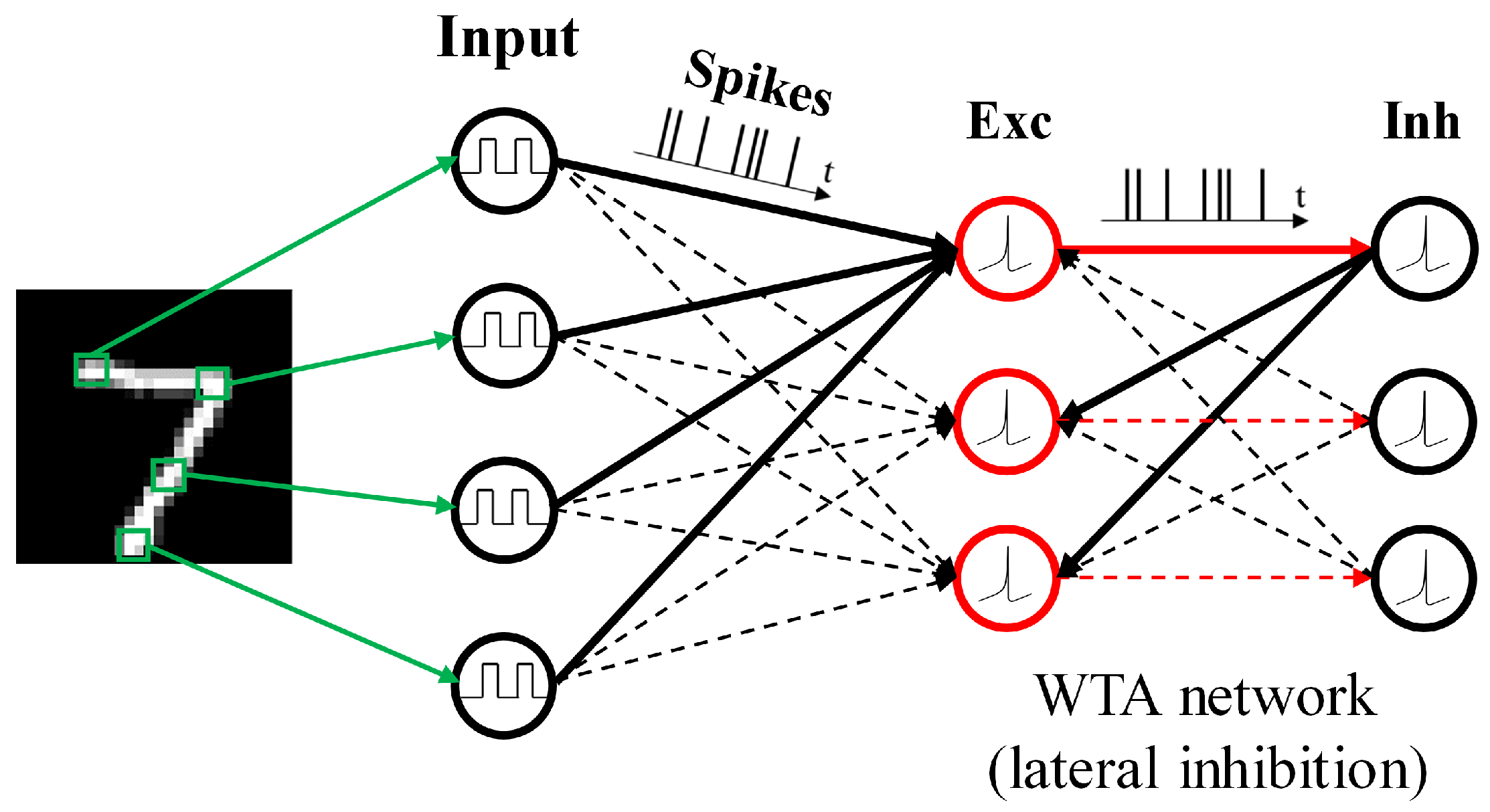
In this paper, the architecture of an SNN is illustrated in Figure 1. The network consists of an input layer and a processing layer. In our experiments, hand-written digit images from the Modified National Institute of Standards and Technology (MNIST) dataset are used as inputs [19]. The dataset is divided into 60,000 training images and 10,000 testing images. The input layer has 784 (28 × 28) neurons which are corresponding to all the pixels in one digit image. Each input neuron produces a Poisson spike train with an arrival rate proportional to the corresponding pixel intensity in the input image. The processing layer is built in a winner-take-all (WTA) network where excitatory neurons are connected to inhibitory neurons in a one-to-one fashion. Each inhibitory neuron sends spikes to all the excitatory neurons except for the one it receives spikes from, which imposes lateral inhibition onto excitatory neurons. The number of excitatory neurons is chosen depending on the required classification accuracy of MNIST dataset, according to [20]. In this work, the networks with 100 and 800 excitatory neurons are selected to study the impact of network size on our proposed methods.
SNNs are usually built with the leaky integrate-and-fire (LIF) neuron models for their simplicity and computational efficiency [3,4,21,22]. The model consists of one first-order linear differential equation that defines the dynamics of membrane potential and a threshold condition that determines the generation of spikes [23]. As for synapses, the conductance-based synaptic model is adopted to transmit information between layers with excitatory and inhibitory ionic channels [20].
Regarding the learning rule, a triplet-based spike-timing-dependent plasticity (STDP) model is considered. The triplet-based STDP model considers three spike traces (one presynaptic trace and two postsynaptic traces) to overcome the limitation of the paired-based STDP models to accommodate the dependence on the repetition frequency of the pairs of spike. It was shown that the triplet rule is more biological plausible where its response can fit the experimental data from the visual cortical slices and hippocampal cultures [24]. In addition, applying triplet-based STDP for unsupervised training of SNNs shows a higher classification accuracy [20]. In addition, a threshold adaption scheme is applied together with the WTA layer to induce the competition for activation among neurons. The model parameters used in the simulation are listed in Table 1. The parameters are configured through an optimization process to achieve the best accuracy. Each time step in the simulation is taken as 0.5 ms. The simulation process of SNNs is carried out in Python program.
2.2. When to Start Neuron Pruning?
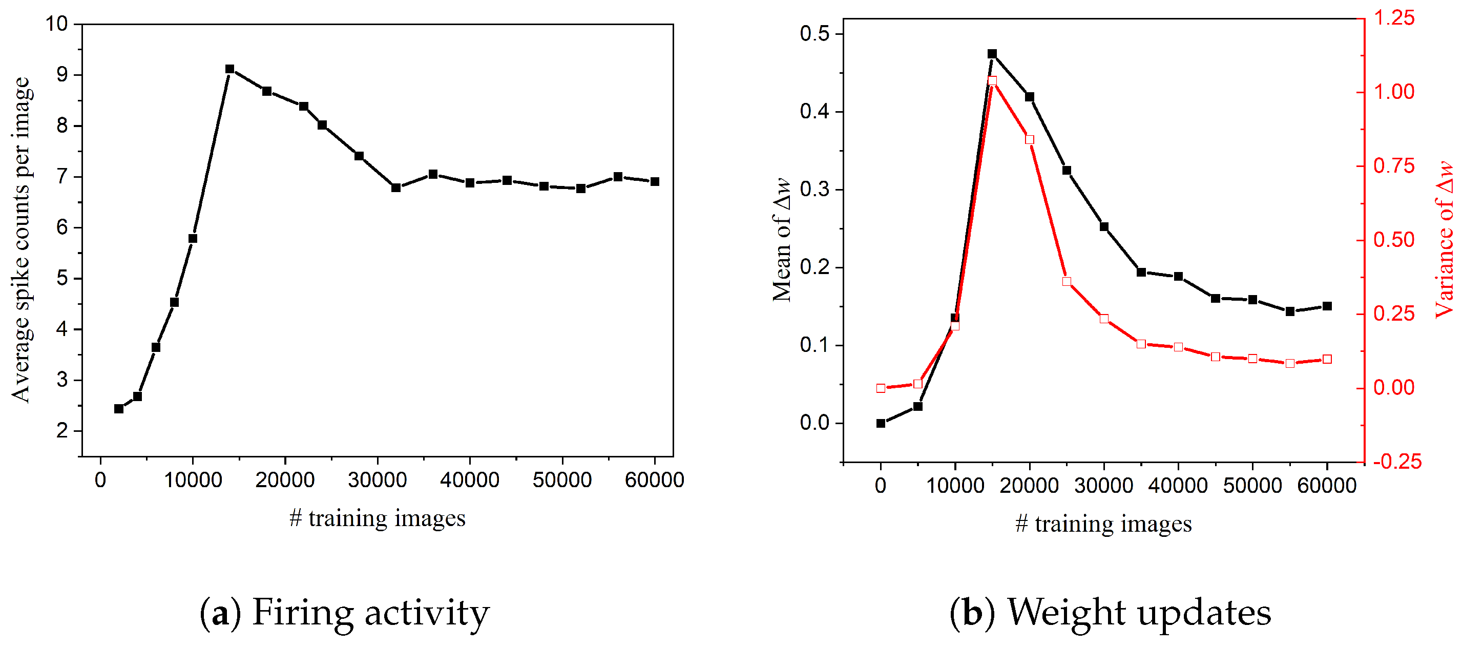
Before delving into the details of neuron pruning, we need to find out when to start the pruning process. If the neuron pruning process starts too early, important neurons that have a profound impact on the output could be mistakenly pruned away, which will deteriorate network performance. On the other hand, if it starts too late, the network might not have enough training cycles to compensate for the accuracy loss. Thus, it is crucial to determine when to start the pruning process. To find this critical point, we have observed how the network dynamics evolve with time by monitoring firing activities and weight updates of output neurons, as shown in Figure 2. Firing activity directly reflects the response of neurons to input patterns. As neurons start to fire regularly after training over 30,000 images, the network has learned the major input features and starts to adjust for small details. This is also confirmed by the statistics of weight updates over time, as shown in Figure 2b. The synchronization happens due to the STDP learning rule that links firing activity and weight updates together. Therefore, we choose to start the neuron pruning process after training over 30,000 images.
2.3. S1: Online Constant Pruning
One of the straightforward ways for neuron pruning is to prune a constant number of neurons after each batch training. Since the firing activity of each neuron directly reflects the response to input patterns, the more frequently one neuron fires, the more features one neuron tends to learn. Thus, the importance of each neuron is determined by its spike counts. Based on this fact, we rank all the output neurons according to their total spike counts during each batch training. And then the n least important neurons will be removed from the network.
2.4. S2: Online Constant-Threshold Pruning
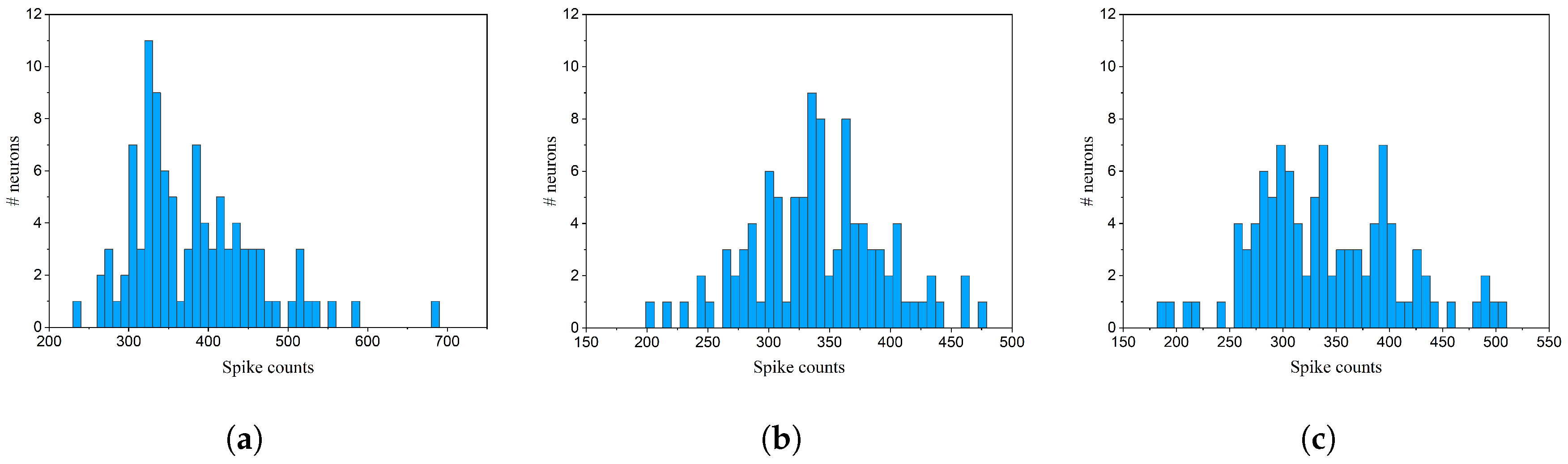
Since firing activity determines the importance of neurons, the neurons to be pruned at each step could be selected according to their spike counts. Therefore, as a second strategy, we propose to define a constant spike count threshold. The spike count threshold is kept constant during the training and applied to select the neurons to be pruned. The pruning process is performed by removing the neurons with spike counts lower than the defined constant threshold after each batch training. However, due to the unsupervised training process, the value of the defined threshold needs to be selected before starting the pruning process in order to achieve different degrees of network size reduction. Thus, the spike count distribution of all the output neurons is measured in the SNN without pruning, as shown in Figure 3. The distribution helps define the range of spike counts and provides us insights to select the value of the threshold before starting the pruning process. From the distributions, it can be observed that the number of spikes fired mainly ranges from 250 to 450. The spike count threshold could be chosen based on the distribution, depending on the percentage of neurons to be pruned.
2.5. S3: Online Adaptive Pruning
The disadvantage of applying a constant threshold is that it can only prune most of the neurons at the beginning of the pruning process. As more neurons are pruned, the neurons that remain will fire more due to less competition. As a result, there will be fewer neurons that can be pruned at later stages due to a constant threshold. This method is not effective when unimportant neurons appear at later stages. Therefore, we propose an adaptive neuron pruning strategy that enables the threshold to be adapted dynamically to the network firing activity. The pruning algorithm is described in Algorithm 1. S2 applies a constant spike count threshold during the pruning process, and the value of the threshold is determined before starting the pruning process. On the other hand, S3 uses an adaptive threshold which changes proportionally with the firing activity, measured during the pruning process. In this pruning strategy, the adaption of the threshold guarantees that a certain percentage of neurons of less importance can be pruned at each pruning step. The choice of the percentage of a is based on the distributions in Figure 3.
| Algorithm 1: Adaptive pruning algorithm |
 |
3. FPGA Implementation
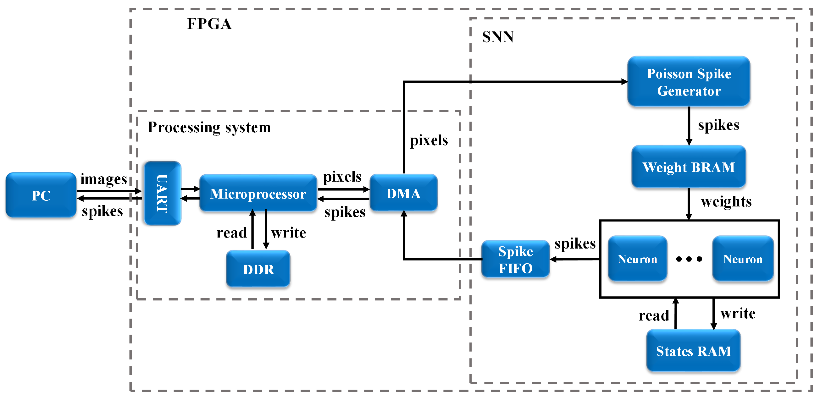
Pruning leads to the reduction of network size and hence improved energy efficiency. To demonstrate the benefit of pruning for hardware implementation, we implemented SNNs after neuron pruning on field programmable gate array (FPGA), and the details of the implementation are presented in this section. Figure 4 shows the proposed digital system for inference. Initially, all the input images are transferred from PC to the external memory (i.e., DDR, SDRAM) on FPGA through a microprocessor using universal asynchronous receiver/transmitter (UART). The microprocessor contains a memory controller which manages the communication between direct memory access (DMA) and the external memory. So image pixels are transferred from the external memory to the network through DMA and converted into Poisson spike trains. The read operations of synaptic weights from block random access memories (BRAMs) are controlled by these spike trains through multiplexing. Then the neuron processing cores update their membrane potentials and generate spikes if the membrane potentials surpass the thresholds. The generated spikes from the SNN are sent out to the external memory and then extracted to PC.
The proposed system is mainly composed of Poisson spikes generator, memory blocks, and neuron processing cores. It is worth mentioning that the proposed pruning strategies ensure a well-structured weight matrix, and hence no additional compression technique is required in the design.
3.1. Poisson Spike Generator
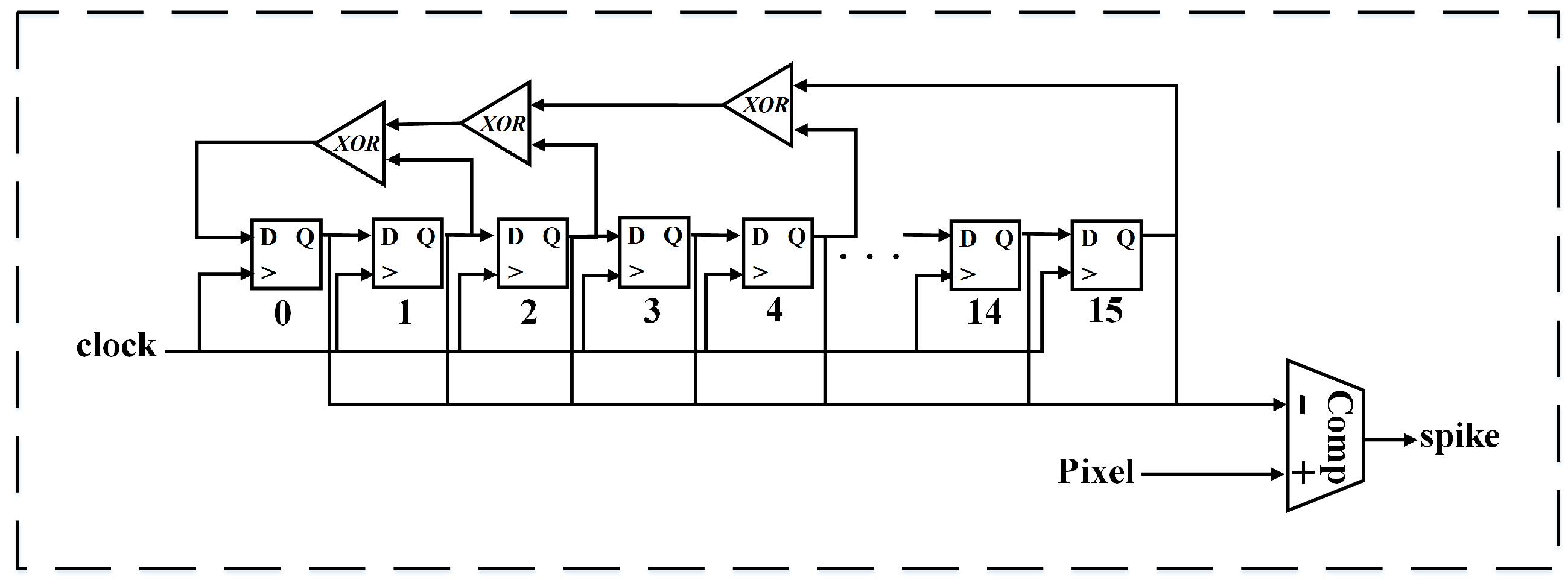
The Poisson spike generator is implemented by comparing input pixel values with a random number that is generated using a 16-bit linear-feedback shift register (LFSR), as shown in Figure 5. Within a particular time window, at each time step, if a pixel value is larger, it outputs a logic-1. Otherwise, it outputs a logic-0. In this way, a Poisson spike train is formed in a time series of 0 and 1.
3.2. Memory Block
In our implementation, the synaptic weights between the input layer and the second layer are stored in the BRAMs, as BRAMs are embedded memory blocks that enable low-power and high-speed near-memory operations inside FPGA fabric. Input spike trains control the access to BRAMs and activate read operations on synaptic weights only if there is an input spike. The synaptic weights accessed from BRAMs are summed and sent into the conductance channel of each excitatory neuron in neuron processing cores.
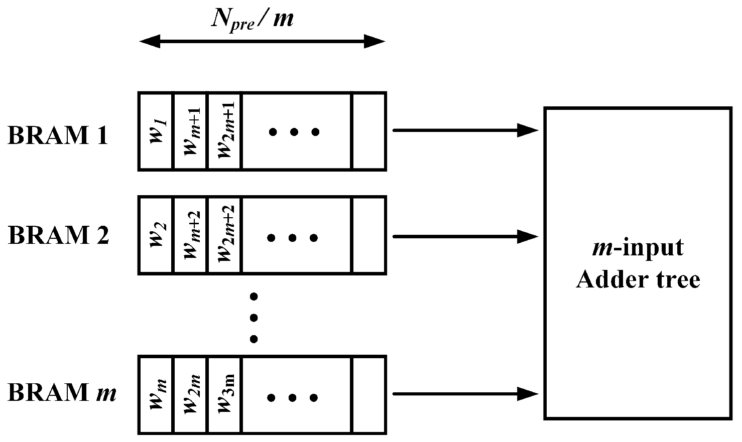
Input spike trains act as the selectors that activate the read operation of the synaptic weights from the BRAMs only if there is an input spike. After that, the selected synaptic weights are summed and sent into the conductance channel of each excitatory neuron in the second layer. This process is equivalent to calculating the accumulation, , where is the synaptic weight between the presynaptic neuron j and the postsynaptic neuron i, is the firing time of the presynaptic neuron j. Because of the fully-connected structure, the accumulation over all the presynaptic neurons j needs to be computed for each postsynaptic neuron i in the second layer. The straightforward implementation is to store all the weights in one single BRAM and read one weight at one time. At each clock cycle, we accumulate one weight sequentially. In this way, it takes around cycles to finish the accumulation, where is the total number of presynaptic neurons in the input layer. However, with a large number of neurons, the accumulation process could take many cycles to complete and hence, slow down the training process. Thus, a parallel design is favoured to accelerate computation. We can divide the synaptic weights associated with one postsynaptic neuron into m BRAMs, as shown in Figure 6, through which m weights are simultaneously read out and passed to m-input adder tree. By pipelining the read and accumulation process, the processing time is taken up by the time for reading the weights and the time for computing the m-input addition. Since the depth of each BRAM becomes , the time for reading the weights is reduced to cycles. As a result, the weights accumulation process can be accelerated significantly. In the implementation, the value of m is selected as 4 to accelerate the process.
3.3. Neuron Processing Core
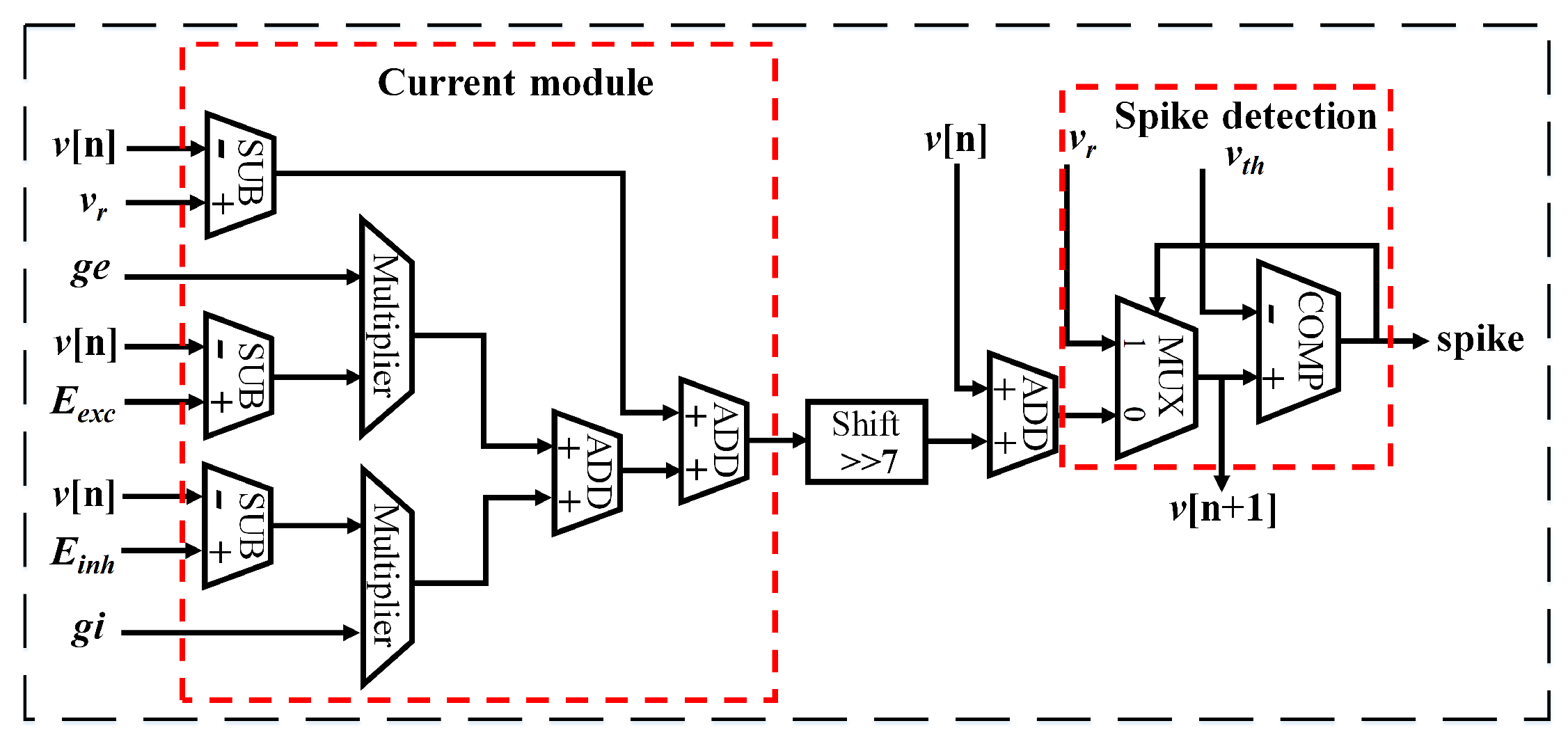
A neuron processing core has two functions, arithmetic computation, and storage of neuron states. The arithmetic computation involves solving differential equations to update state variables of a neuron, like synaptic conductance and membrane potential. The implementation of the arithmetic unit is based on the Euler method, as shown in Figure 7 [25]. First, the current module generates the synaptic current and leakage current by multiplying the synaptic conductances with the voltage drop. Then the membrane potential is updated by integrating the synaptic currents and compared with the threshold voltage. An output spike will be detected once the membrane potential surpasses the threshold. In the design, the multiplications between the conductance and voltage drops are implemented by multipliers. The multiplication by constants is realized by shift operation by properly choosing the constants as powers of two. In addition, each core provides a memory space for storing the state variables, including membrane potential, synaptic conductance, and threshold potential.
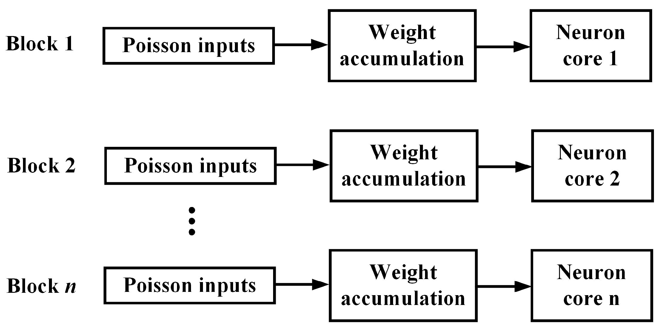
A parallel implementation scheme for neuron processing cores is depicted in Figure 8, where n neuron processing cores are implemented and the membrane potentials of the n neurons are updated in parallel. Each neuron core receives the accumulated synaptic weights read out from BRAMs controlled by input spike trains. By using the time-multiplexing design, we can update the membrane potentials of all the output neurons in stages, where is the total number of output neurons. Within one step of the time-multiplexing process, the membrane potential of n neurons can be updated in parallel.
4. Results and Discussion
4.1. Network Performance
To gain insight into the performance of the proposed techniques, we study two sample unpruned SNN networks. The first is trained with 100 output neurons, while the second is trained with 800 output neurons. The accuracy achieved using the network described in Section 2.1 was 85.78%/90.4% respectively. The performance of the proposed pruning strategies and comparisons among them are discussed in the following sections. All the results are obtained from the simulation of the SNN described in Section 2.1.
4.1.1. Online Pruning
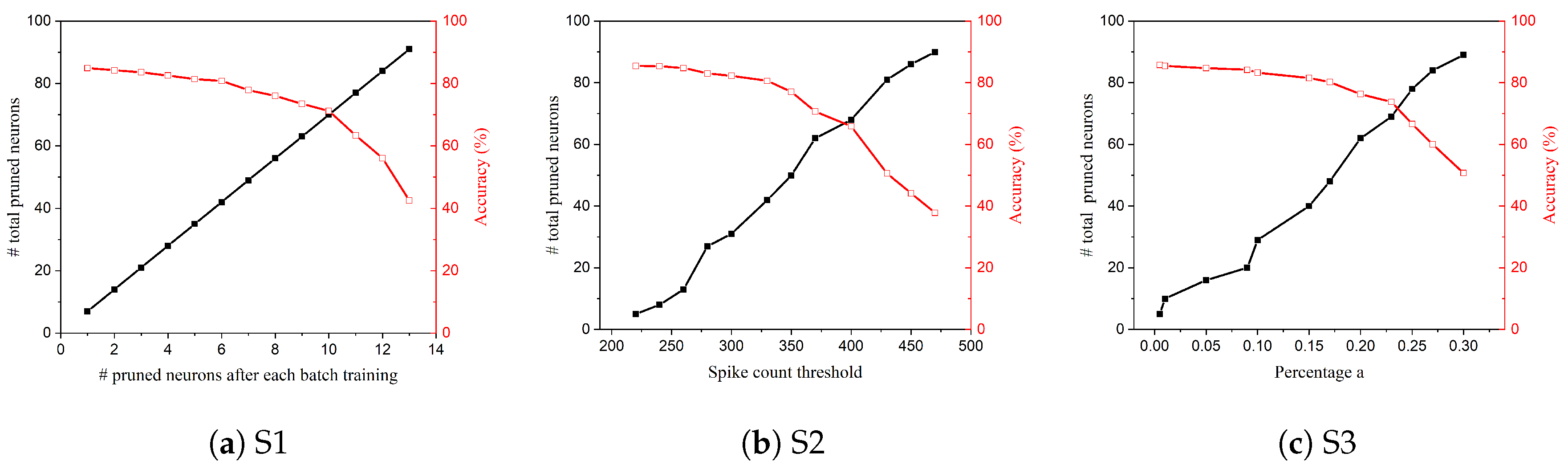
Pruning performance results for the proposed pruning techniques are shown in Figure 9, presenting that the total number of pruned neurons and classification accuracy change with the corresponding control variables, i.e., constant number, spike count threshold, and percentage respectively. In Figure 9a, the total number of pruned neurons grows linearly with a constant number. Consequently, the classification accuracy decreases as more neurons are pruned. Figure 9b,c show similar observations except that the total number of pruned neurons increases non-linearly. More importantly, these results provide guidelines for how to determine the value of corresponding control variables to obtain the desired network size and classification accuracy at the end. The choice should be based on the consideration of the trade-off between classification accuracy and energy efficiency.
4.1.2. Comparison: 100 Output Neurons
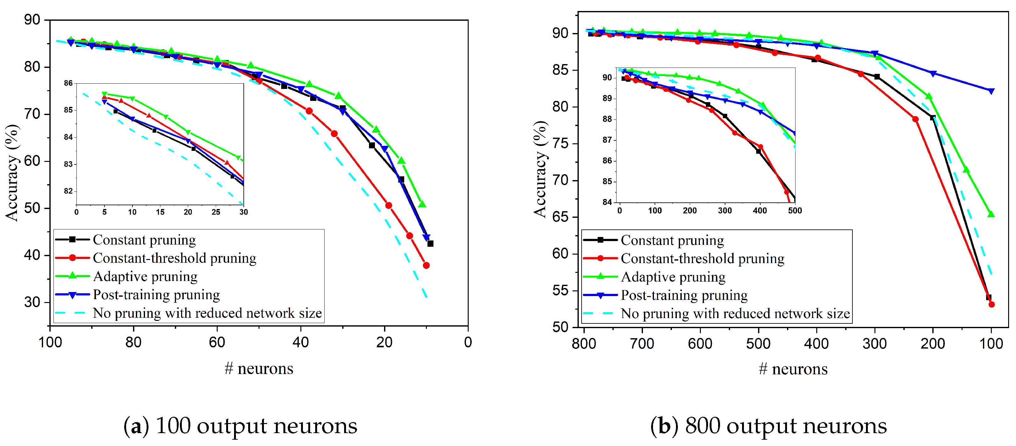
In order to provide a comparative framework for performance evaluation, we compare the proposed approaches to each other and to a post-training pruning method that was reported in [16]. The post-training pruning method is described as follows. After training, 10,000 images chosen from the training dataset are given as inputs to the trained SNN, and membrane potential and firing activity of each neuron are monitored. Output neurons are then ranked according to their average spike counts. The least important neurons are pruned. Comparisons between different approaches are based on the number of pruned neurons, as discussed in the next subsections.
Figure 10a shows more detailed comparisons among different pruning strategies in the SNN with 100 output neurons. The no pruning method with reduced network size corresponds to the case where unpruned SNNs are trained with the given number of output neurons (x-axis in the figure). Training parameters such as time constants, learning rates for STDP etc. are kept constant, as referenced to the SNN with 100 output neurons. Clearly, when more than 50 neurons are pruned, the proposed pruning methods show better results than the no pruning method, which implies that pruning is able to get rid of unimportant neurons that also classify many wrong digits and hence contribute negatively to overall accuracy. This observation suggests that through pruning methods, the network is able to achieve higher accuracy than that obtained by no pruning for the same network size. Moreover, among the proposed pruning methods, the constant pruning method gives the worst results, especially when more than 50 neurons are pruned. The adaptive pruning method shows slightly better results than the constant-threshold pruning method because the pruning threshold is adapted to the network dynamics, and hence only the least important neurons will be pruned at each step. Compared with post-training pruning method, the adaptive pruning method also shows better performance because online pruning provides more opportunities for unpruned important neurons to learn more input features by removing unimportant neurons from the network. With adaptive pruning method, when 16 neurons are pruned, the accuracy loss was only 1%.
4.1.3. Comparison: 800 Output Neurons
Furthermore, the proposed pruning strategies were also applied in the SNN with 800 output neurons, and the comparisons are shown in Figure 10b. In this case, the adaptive pruning method provides slightly better performance than the no pruning method with reduced network size. Adaptive pruning method is also proven to be a better approach than the other proposed online pruning strategies. However, compared with post-training pruning, when the number of pruned neurons is more than 500, adaptive pruning causes much more severe accuracy drop. Another interesting observation is that constant pruning and constant-threshold pruning methods both show worse results than the no pruning method, which suggests that it is important to prune neurons according to the network dynamics, especially in a large network where the difference among all the neurons becomes small. Therefore, it is further confirmed that adaptive pruning is a simple and effective pruning method. And the benefit of adaptive pruning method becomes more prominent in a larger network. The accuracy loss is still within 1% when 300 neurons are pruned.
Table 2 summarizes the classification accuracy for SNNs with different network size (100 and 800 output neurons) after applying different pruning strategies. Clearly, the unpruned SNN with 100 (800) neurons produces the best accuracy. With neurons being pruned, the adaptive pruning method leads to the smallest accuracy loss, also outperforming post-training pruning method. This suggests the significant potential of adaptive pruning method in online training systems as it can improve training energy efficiency and maintain high classification accuracy.
4.2. FPGA Implementation Results
In our digital implementation, Xilinx Vivado Design Suite was used to program and simulate the proposed digital system in Verilog hardware description language (HDL). The Verilog code was then synthesized and implemented on the Xilinx Virtex-7 VC709 evaluation board for verification. Power consumption was obtained after routing by using the power analysis tool in Vivado Design Suite, which provides detailed analysis and accurate estimation [26]. The implemented SNNs run at 100 MHz clock frequency. The number of physical neurons placed inside the FPGA is chosen as 25 for optimum energy efficiency, so time-division multiplexing is utilized to run the whole network. To avoid overflow and severe precision loss in fixed-point arithmetic, 16 integer bits and nine fraction bits are chosen.
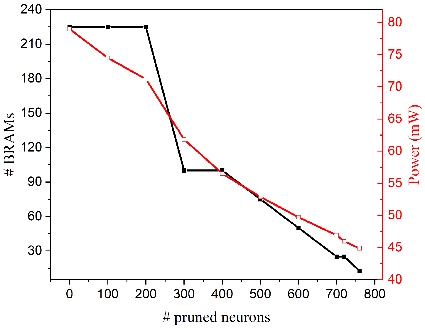
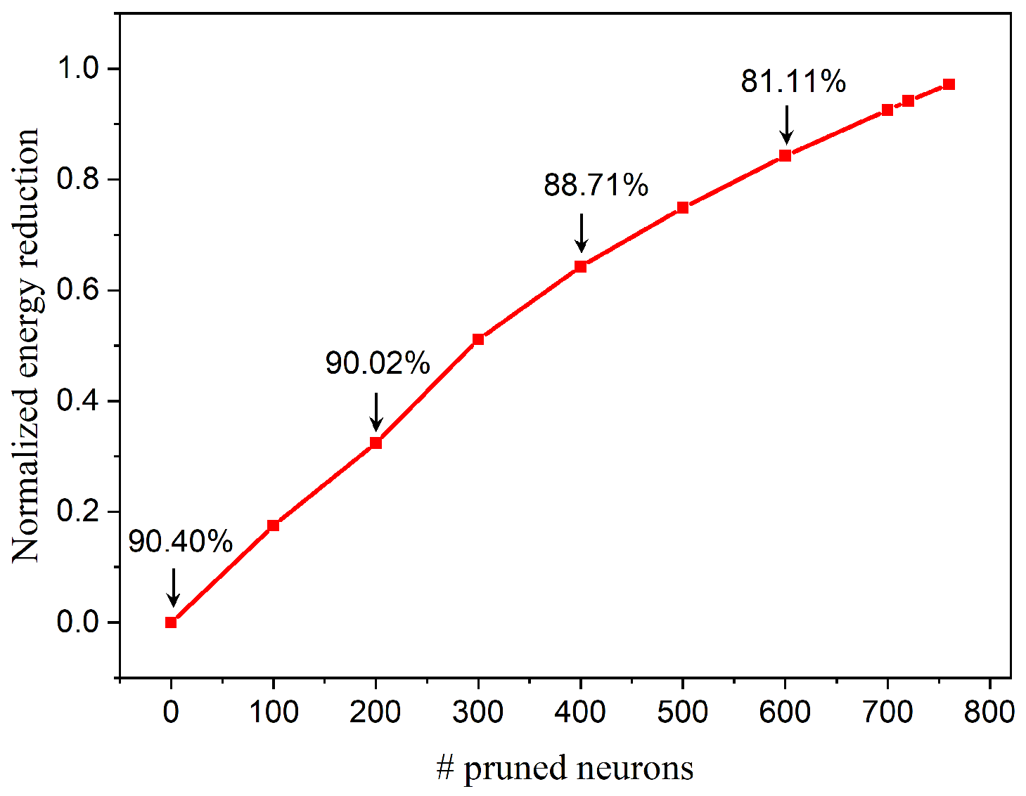
Neuron pruning directly reduces the network size by removing entire neurons. In order to demonstrate the impact of neuron pruning on hardware and energy savings, an FPGA realization is designed for inference only. The pruned model parameters are transferred to the FPGA where the evaluation is performed. Figure 11 shows the number of BRAMs required for storing synaptic weights and power consumption for the different number of pruned neurons in the SNN with 800 output neurons initially. On FPGA, BRAMs are synthesized by arranging memory primitives together for optimized performance. It can be seen that the number of BRAMs remains the same initially before it drops by 56% when 300 or 400 neurons are pruned. When more than 400 neurons are pruned, the required memory size starts to decrease linearly. On the other hand, power consumption goes down continuously with the number of pruned neurons. Since the implementation of neuron cores on the FPGA remains unchanged, the power reduction is mainly caused by the reduced operations on memory when neurons are pruned. Moreover, the energy consumption for processing one image is estimated in terms of runtime and power consumption. Accordingly, we define the normalized energy reduction as , where is the energy consumption of the SNN without pruning, and is the energy consumption after pruning n neurons, as shown in Figure 12. Because of parallel implementation, the runtime for processing one image decreases linearly with the number of pruned neurons. Therefore, energy reduction goes up almost linearly with the number of pruned neurons because runtime improvement is more significant than power reduction. Moreover, from both Figure 11 and Figure 12, it can be seen that with pruning, the benefit of memory and energy reduction is significant while the accuracy loss remains small. For example, when 400 neurons are pruned, the memory size and energy are decreased by around 56% and 64% respectively, while the accuracy loss is only 1.69%. Different pruning percentage will lead to different results, and the choice depends on the trade-off among accuracy, memory, and energy consumption. Our study provides a clear guideline for how to reduce network complexity to gain memory and energy reduction benefits and mitigate accuracy loss.
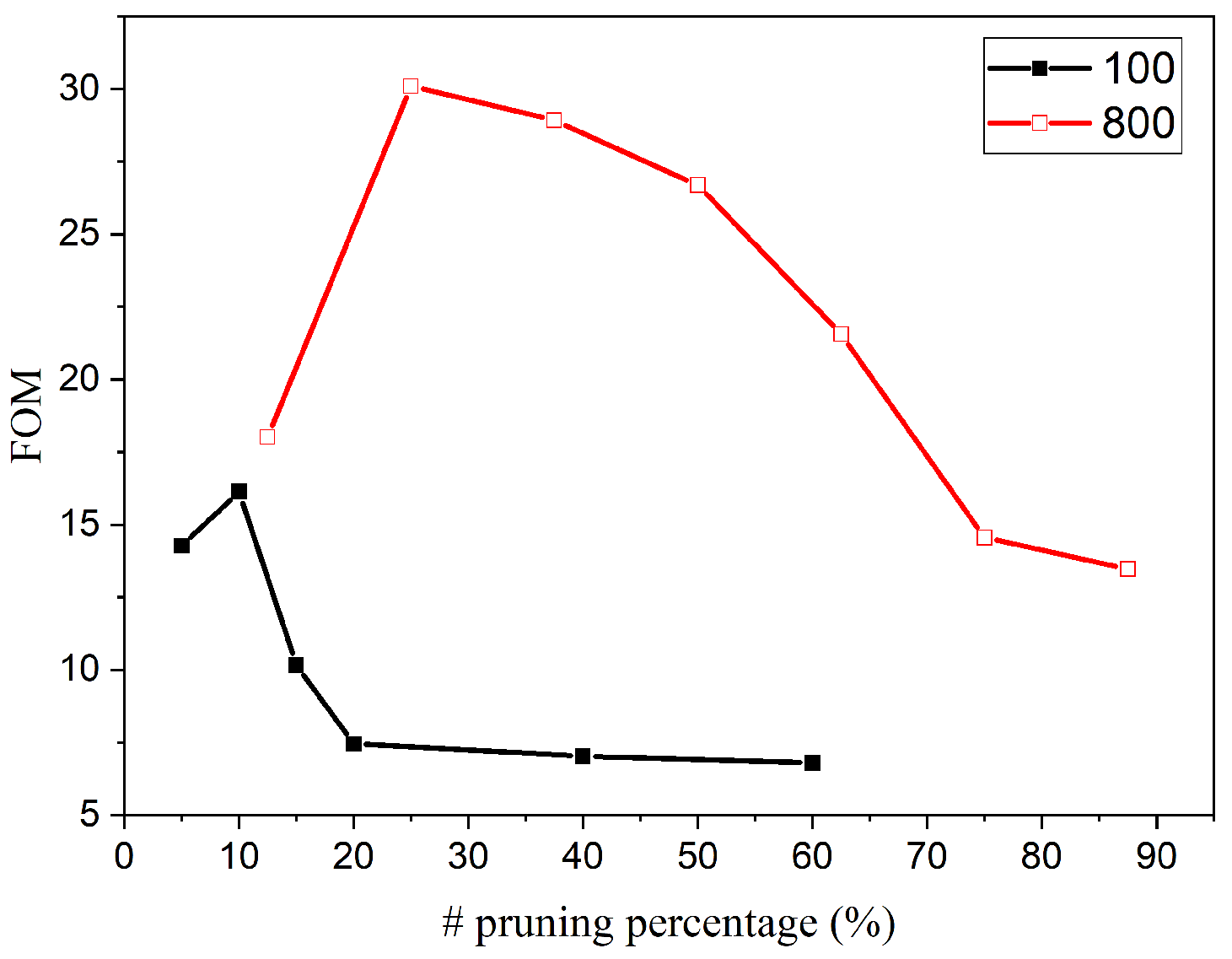
To help choose pruning percentage, we define a figure of merit (FOM) as below by considering network size, accuracy loss, and energy.
where accuracy loss is defined as the accuracy difference between the networks without pruning and with pruning, the energy is measured in mJ, and all the variables in the equation are normalized to the corresponding maximum value. The defined FOM is used on a per network basis to help identify the best pruning percentage for that specific network as demonstrated in Figure 13. According to the defined FOM, the best choices are at 10% and 25% for networks with 100 and 800 output neurons, respectively. It should be noted that the proposed FOM provides one way to determine the best pruning percentage, and other definitions could also be applied depending on the requirements for specific applications.
5. Conclusions
This paper proposes three different strategies for pruning neurons while training in an unsupervised spiking neural network and a parallel digital implementation scheme on FPGA. Neuron online pruning provides an efficient approach for reducing network complexity and significant benefits for hardware implementation. The proposed methods exploit network dynamics to rank output neurons and remove unimportant ones. It is demonstrated that online pruning with an adaptive spike count threshold, shows the best performance over other proposed methods. Adaptive pruning method also shows better performance than post-training pruning, which suggests that adaptive online pruning can not only improve training energy efficiency but also achieve higher accuracy. Furthermore, the adaptive pruning method is proven to be a simple and effective approach that leads to higher classification accuracy compared with the no pruning method with reduced network size (i.e., the SNNs trained with less than the initial 100 (or 800) neurons and without pruning). The effectiveness of our methods is also verified in SNNs with different network size, and it provides a clear insight into the trade-off between classification accuracy and network complexity. With adaptive pruning method, when 300 neurons are pruned from the 800-neuron network, the accuracy loss is still less than 1%. Moreover, the pruned networks were implemented on FPGA in a parallel architecture. The implementation architecture is scalable and can be directly applied to different pruned SNNs as our proposed pruning strategies preserve a well-structured weight matrix. The implementation results have shown a 2.3× reduction in memory size and 2.8× on energy consumption when 400 neurons are pruned. In addition, a figure of merit is proposed to help identify the best choice of pruning percentage for different network size. Therefore, the proposed adaptive neuron pruning strategy provides a promising approach for reducing memory size and improving energy efficiency with high accuracy in spike neural networks for real-time applications.
Author Contributions
Conceptualization, W.G. and H.E.Y.; methodology, W.G.; software, W.G.; validation, W.G., H.E.Y. and M.E.F.; investigation, W.G., H.E.Y. and M.E.F.; writing—original draft preparation, W.G.; writing—review and editing, H.E.Y., M.E.F., A.M.E. and K.N.S.; supervision, A.M.E. and K.N.S.; project administration, K.N.S. All authors have read and agreed to the published version of the manuscript.
Funding
This research received no external funding.
Acknowledgments
We acknowledge the financial support from King Abdullah University of Science and Technology (KAUST), Saudi Arabia.
Conflicts of Interest
The authors declare no conflict of interest.
References
- Grossfeld, R.M. An Introduction to Nervous Systems. Ralph J. Greenspan, editor. Integr. Comp. Biol. 2008, 48, 439–441. [Google Scholar] [CrossRef]
- Furber, S.B.; Galluppi, F.; Temple, S.; Plana, L.A. The SpiNNaker Project. Proc. IEEE 2014, 102, 652–665. [Google Scholar] [CrossRef]
- Davies, M.; Srinivasa, N.; Lin, T.; Chinya, G.; Cao, Y.; Choday, S.H.; Dimou, G.; Joshi, P.; Imam, N.; Jain, S.; et al. Loihi: A Neuromorphic Manycore Processor with On-Chip Learning. IEEE Micro 2018, 38, 82–99. [Google Scholar] [CrossRef]
- Merolla, P.A.; Arthur, J.V.; Alvarez-Icaza, R.; Cassidy, A.S.; Sawada, J.; Akopyan, F.; Jackson, B.L.; Imam, N.; Guo, C.; Nakamura, Y.; et al. A million spiking-neuron integrated circuit with a scalable communication network and interface. Science 2014, 345, 668–673. [Google Scholar] [CrossRef] [PubMed]
- Tavanaei, A.; Ghodrati, M.; Kheradpisheh, S.R.; Masquelier, T.; Maida, A. Deep learning in spiking neural networks. Neural Netw. 2019, 111, 47–63. [Google Scholar] [CrossRef] [PubMed] [Green Version]
- Kolb, B.; Whishaw, I.Q. Fundamentals of Human Neuropsychology, 5th ed.; Worth Publishers: New York, NY, USA, 2003. [Google Scholar]
- Zillmer, E.; Spiers, M.; Culbertson, W. Principles of Neuropsychology; Thomson Wadsworth: Belmont, CA, USA, 2008. [Google Scholar]
- Han, S.; Pool, J.; Tran, J.; Dally, W.J. Learning Both Weights and Connections for Efficient Neural Networks. In Proceedings of the 28th International Conference on Neural Information Processing Systems, Montreal, QC, Canada, 7–12 December 2015; pp. 1135–1143. [Google Scholar]
- Yu, J.; Lukefahr, A.; Palframan, D.; Dasika, G.; Das, R.; Mahlke, S. Scalpel: Customizing DNN pruning to the underlying hardware parallelism. In Proceedings of the 2017 ACM/IEEE 44th Annual International Symposium on Computer Architecture (ISCA), Toronto, ON, Canada, 24–28 June 2017; pp. 548–560. [Google Scholar] [CrossRef]
- Hu, H.; Peng, R.; Tai, Y.W.; Tang, C.K. Network Trimming: A Data-Driven Neuron Pruning Approach towards Efficient Deep Architectures. arXiv 2016, arXiv:1607.03250. [Google Scholar]
- Li, H.; Kadav, A.; Durdanovic, I.; Samet, H.; Graf, H.P. Pruning Filters for Efficient ConvNets. arXiv 2016, arXiv:1608.08710. [Google Scholar]
- Moya Rueda, F.; Grzeszick, R.; Fink, G.A. Neuron Pruning for Compressing Deep Networks Using Maxout Architectures. In Pattern Recognition; Roth, V., Vetter, T., Eds.; Springer International Publishing: Cham, Switzerland, 2017; pp. 177–188. [Google Scholar] [CrossRef] [Green Version]
- Luo, J.H.; Wu, J.; Lin, W. ThiNet: A Filter Level Pruning Method for Deep Neural Network Compression. In Proceedings of the 2017 IEEE International Conference on Computer Vision (ICCV), Venice, Italy, 22–29 October 2017; pp. 5068–5076. [Google Scholar] [CrossRef] [Green Version]
- Molchanov, P.; Mallya, A.; Tyree, S.; Frosio, I.; Kautz, J. Importance Estimation for Neural Network Pruning. In Proceedings of the 2019 IEEE/CVF Conference on Computer Vision and Pattern Recognition (CVPR), Long Beach, CA, USA, 16–21 June 2019; pp. 11256–11264. [Google Scholar] [CrossRef] [Green Version]
- Dora, S.; Sundaram, S.; Sundararajan, N. A two stage learning algorithm for a Growing-Pruning Spiking Neural Network for pattern classification problems. In Proceedings of the 2015 International Joint Conference on Neural Networks (IJCNN), Killarney, Ireland, 12–16 July 2015; pp. 1–7. [Google Scholar] [CrossRef]
- Chen, R.; Ma, H.; Xie, S.; Guo, P.; Li, P.; Wang, D. Fast and Efficient Deep Sparse Multi-Strength Spiking Neural Networks with Dynamic Pruning. In Proceedings of the 2018 International Joint Conference on Neural Networks (IJCNN), Rio de Janeiro, Brazil, 8–13 July 2018; pp. 1–8. [Google Scholar] [CrossRef]
- Dimovska, M.; Johnston, T.; Schuman, C.D.; Mitchell, J.P.; Potok, T.E. Multi-Objective Optimization for Size and Resilience of Spiking Neural Networks. In Proceedings of the 2019 IEEE 10th Annual Ubiquitous Computing, Electronics Mobile Communication Conference (UEMCON), New York, NY, USA, 10–12 October 2019; pp. 0433–0439. [Google Scholar] [CrossRef] [Green Version]
- Wu, D.; Lin, X.; Du, P. An Adaptive Structure Learning Algorithm for Multi-Layer Spiking Neural Networks. In Proceedings of the 2019 15th International Conference on Computational Intelligence and Security (CIS), Macau, China, 13–16 December 2019; pp. 98–102. [Google Scholar] [CrossRef]
- Lecun, Y.; Bottou, L.; Bengio, Y.; Haffner, P. Gradient-based learning applied to document recognition. Proc. IEEE 1998, 86, 2278–2324. [Google Scholar] [CrossRef] [Green Version]
- Diehl, P.; Cook, M. Unsupervised learning of digit recognition using spike-timing-dependent plasticity. Front. Comput. Neurosci. 2015, 9, 99. [Google Scholar] [CrossRef] [PubMed] [Green Version]
- Frenkel, C.; Lefebvre, M.; Legat, J.; Bol, D. A 0.086-mm2 12.7-pJ/SOP 64k-Synapse 256-Neuron Online-Learning Digital Spiking Neuromorphic Processor in 28-nm CMOS. IEEE Trans. Biomed. Circuits Syst. 2019, 13, 145–158. [Google Scholar] [CrossRef] [Green Version]
- Detorakis, G.; Sheik, S.; Augustine, C.; Paul, S.; Pedroni, B.U.; Dutt, N.; Krichmar, J.; Cauwenberghs, G.; Neftci, E. Neural and Synaptic Array Transceiver: A Brain-Inspired Computing Framework for Embedded Learning. Front. Neurosci. 2018, 12, 583. [Google Scholar] [CrossRef] [PubMed]
- Burkitt, N. A Review of the Integrate-and-Fire Neuron Model: I. Homogeneous Synaptic Input. Biol. Cybern. 2006, 95, 1–19. [Google Scholar] [CrossRef] [PubMed]
- Pfister, J.P.; Gerstner, W. Triplets of spikes in a model of spike timing-dependent plasticity. J. Neurosci. 2006, 26, 9673–9682. [Google Scholar] [CrossRef] [PubMed] [Green Version]
- Atkinson, K.E.; Han, W.; Stewart, D. Euler’s method. In Numerical Solution of Ordinary Differential Equations; John Wiley & Sons, Ltd.: Hoboken, NJ, USA, 2011; Chapter 2; pp. 15–36. [Google Scholar] [CrossRef]
- Muslim, F.B.; Ma, L.; Roozmeh, M.; Lavagno, L. Efficient FPGA Implementation of OpenCL High-Performance Computing Applications via High-Level Synthesis. IEEE Access 2017, 5, 2747–2762. [Google Scholar] [CrossRef]
Figure 1.
The architecture of a spiking neural network (SNN). The network consists of an input layer and a processing layer that is based on a winner-take-all (WTA) network with excitatory (Exc) neurons connected with inhibitory (Inh) neurons to induce lateral inhibition. An example image of digit 7 is taken from MNIST dataset.

Figure 2.
Network dynamics changing with time in the SNN with 100 output neurons and no pruning. The results are obtained from the simulation described in Section 2.1. (a) Firing activity. The average of spike counts of 100 output neurons was monitored every 2000 training images. (b) Statistics of weight updates Dw. The mean (black) and variance (red) were calculated every 5000 training images.

Figure 3.
The distributions of spike counts after training over different number of images measured in the SNN with 100 output neurons and no pruning. The results are obtained from the simulation described in Section 2.1. (a) 30,000 training images; (b) 45,000 training images; (c) 60,000 training images

Figure 4.
The proposed digital system of an SNN for inference.

Figure 5.
The digital implementation of Poisson spike generator.

Figure 6.
The memory allocation of synaptic weights in BRAMs and parallel structures for one neuron core. is the number of the presynaptic neurons in the input layer. Synaptic weights associated with one neuron are stored in m BRAMs. So m weights can be read at the same time and sent to the adder tree for accumulation.

Figure 7.
The digital implementation of leaky integrate-and-fire (LIF) neuron model. The design is based on Euler method. and are the membrane potential at time n and respectively. is the rest potential. is the threshold potential. and are the excitatory and inhibitory synaptic conductance respectively. and are the reverse potentials of the excitatory and inhibitory synapse respectively. The current module produces the input synaptic current. The spike detection module checks the occurrence of an output spike.

Figure 8.
Parallel implementation scheme for neuron processing cores. Poisson spike trains converted from input pixels allow corresponding synaptic weights to be read out from BRAMs and accumulated before being sent into neuron processing cores. n neurons processing cores are updated in parallel.
Figure 8.
Parallel implementation scheme for neuron processing cores. Poisson spike trains converted from input pixels allow corresponding synaptic weights to be read out from BRAMs and accumulated before being sent into neuron processing cores. n neurons processing cores are updated in parallel.

Figure 9.
The total number of pruned neurons and classification accuracy for online pruning strategies. (a) S1: constant pruning, (b) S2: constant-threshold pruning, and (c) S3: adaptive pruning.
Figure 9.
The total number of pruned neurons and classification accuracy for online pruning strategies. (a) S1: constant pruning, (b) S2: constant-threshold pruning, and (c) S3: adaptive pruning.

Figure 10.
Comparisons among different pruning strategies for (a) 100 output neurons, and (b) 800 output neurons.
Figure 10.
Comparisons among different pruning strategies for (a) 100 output neurons, and (b) 800 output neurons.

Figure 11.
Number of BRAMs and power consumption for the SNN with different number of pruned neurons. The initial network size is of 800 output neurons.
Figure 11.
Number of BRAMs and power consumption for the SNN with different number of pruned neurons. The initial network size is of 800 output neurons.

Figure 12.
Energy reduction for the SNN with different numbers of pruned neurons. The initial network size is of 800 output neurons. The energy reduction is estimated for processing one image. Accuracy is displayed for 0, 200, 400, and 600 pruned neurons respectively.
Figure 12.
Energy reduction for the SNN with different numbers of pruned neurons. The initial network size is of 800 output neurons. The energy reduction is estimated for processing one image. Accuracy is displayed for 0, 200, 400, and 600 pruned neurons respectively.

Figure 13.
Figure of merit at different pruning percentage for both cases of 100 and 800 output neurons.
Figure 13.
Figure of merit at different pruning percentage for both cases of 100 and 800 output neurons.


Table 1.
Model parameters used in the simulation. During the simulation, the unit for the time constants is ms, and the unit for the threshold adaption constant is mV.
Table 1.
Model parameters used in the simulation. During the simulation, the unit for the time constants is ms, and the unit for the threshold adaption constant is mV.
| Parameters | Value |
|---|---|
| The time constant for membrane potential update | 100 |
| The time constant for the presynaptic trace in the STDP model | 4 |
| The time constants for fast and slow postsynaptic traces in the STDP model respectively | 8, 16 |
| The time constant for the excitatory conductance | 1 |
| The time constant for the inhibitory conductance | 2 |
| The learning rates for presynaptic and postsynaptic update in the STDP model respectively | 0.0001, 0.01 |
| Threshold adaption constant | 0.01 |
Table 2.
Comparison among different pruning strategies. For no pruning method, accuracy is obtained for SNNs with 100 and 800 output neurons respectively. For other pruning methods, accuracy is obtained for pruned SNNs with initially 100 and 800 output neurons respectively. Post-training pruning method is adopted from [16].
| Methods | Accuracy (%) (100/800) | # Pruned Neurons (100/800) |
|---|---|---|
| No pruning | 85.78/90.4 | 0 |
| Constant pruning | 83.69/88.18 | 20/300 |
| Constant-threshold pruning | 83.89/87.89 | 20/300 |
| Adaptive pruning | 84.21/89.58 | 20/300 |
| Post-training pruning | 83.88/88.94 | 20/300 |
© 2020 by the authors. Licensee MDPI, Basel, Switzerland. This article is an open access article distributed under the terms and conditions of the Creative Commons Attribution (CC BY) license (http://creativecommons.org/licenses/by/4.0/).
Share and Cite
MDPI and ACS Style
Guo, W.; Yantır, H.E.; Fouda, M.E.; Eltawil, A.M.; Salama, K.N. Towards Efficient Neuromorphic Hardware: Unsupervised Adaptive Neuron Pruning. Electronics 2020, 9, 1059. https://0-doi-org.brum.beds.ac.uk/10.3390/electronics9071059
AMA Style
Guo W, Yantır HE, Fouda ME, Eltawil AM, Salama KN. Towards Efficient Neuromorphic Hardware: Unsupervised Adaptive Neuron Pruning. Electronics. 2020; 9(7):1059. https://0-doi-org.brum.beds.ac.uk/10.3390/electronics9071059
Chicago/Turabian StyleGuo, Wenzhe, Hasan Erdem Yantır, Mohammed E. Fouda, Ahmed M. Eltawil, and Khaled Nabil Salama. 2020. "Towards Efficient Neuromorphic Hardware: Unsupervised Adaptive Neuron Pruning" Electronics 9, no. 7: 1059. https://0-doi-org.brum.beds.ac.uk/10.3390/electronics9071059
Note that from the first issue of 2016, this journal uses article numbers instead of page numbers. See further details here.