Neural Network-Based Aircraft Conflict Prediction in Final Approach Maneuvers

Abstract

Conflict detection and resolution is one of the main topics in air traffic management. Traditional approaches to this problem use all the available information to predict future aircraft trajectories. In this work, we propose the use of a neural network to determine whether a particular configuration of aircraft in the final approach phase will break the minimum separation requirements established by aviation rules. To achieve this, the network must be effectively trained with a large enough database, in which configurations are labeled as leading to conflict or not. We detail the way in which this training database has been obtained and the subsequent neural network design and training process. Results show that a simple network can provide a high accuracy, and therefore, we consider that it may be the basis of a useful decision support tool for both air traffic controllers and airborne autonomous navigation systems.

1. Introduction

This work is part of a line of research aimed at improving air traffic management (ATM) procedures. More specifically, the line focuses on improving operations in the airport environment, and it is mainly motivated by the relentless increase in global air traffic [1].

All proposals in this field must thoroughly respect the vast rules issued by the many civil aviation authorities in this sector. These authorities include the ICAO (International Civil Aviation Organization), a United Nations agency, which promotes aviation safety and the orderly development of international civil aviation worldwide. The ICAO establishes standards and regulations necessary for aviation safety, efficiency, regulation, and for environmental protection. One of the many safety requirements that air operations must meet has to do with maintaining a minimum lateral and vertical separation between aircraft that are in flight. For example, the minimum lateral separation is 5 NM (we use nautical miles (NM), feet (ft), and knots (kt), as they are usual units of measurement in air navigation. In the International System of Units (SI), 1 NM = 1852 m, 1 ft = 0.3048 m, and 1 kt = 0.5144 m/s) for en-route airspace, and 3 NM inside the terminal radar approach control area. On the other hand, the minimum vertical separation is 2000 ft above 29,000 ft, and 1000 ft below this altitude [2].

Air traffic conflict detection and resolution (CD and R) mechanisms [3,4] aim to maintain the separation between in-flight aircraft established by the aviation regulation. In this context, a “conflict” (or “collision”) is an event in which two or more aircraft experience a loss of minimum separation. Traditional CD and R mechanisms use some geometric [5,6,7] or probabilistic [8,9,10] techniques for predicting future aircraft trajectories starting from, for example, known flight plans or current radar information. Trajectory prediction allows the detection of conflict in advance and the triggering of actions to prevent it from happening.

According to the prediction horizon, CD and R mechanisms can be classified into three categories: Long-term CD and R (horizons over 30 min), medium-term CD and R (horizons up of to 30 min), and short-term CD and R (horizons up of to 10 min). In this work, we focus on short-term CD and R. At this level, there are ground-based systems that assist air controllers. They use information from surveillance radars or other, more advanced systems, such as the Automatic Dependent Surveillance—Broadcast (ADS-B) system [11]. One example of a ground-based CD and R system is the Short-Term Conflict Alert (STCA) [12]. On the other hand, there is a family of airborne devices that function independently from the ground-based Air Traffic Control (ATC) system. This is the case of the Traffic Collision Avoidance System (TCAS) [13]. In this case, conflict is detected by establishing a direct communication between nearby aircraft. In [14], conflict resolution for autonomous aircraft in the medium and short terms is investigated.

On the other hand, neural networks [15] are quickly growing in popularity, mainly due to the great advances that are being made in terms of computing power. Thanks to this and the proliferation of the development of graphic accelerators, which have proven quite capable for the training process of these networks, more and more uses are being raised for this technology, which requires long and costly training in computing terms, but exhibits a high efficiency after the networks are trained.

In this context, the present work explores the possibility of using a neural network to detect in advance the breach of the requirement of minimum separation between aircraft. In particular, we focus on the prediction of conflicts during the approach flight phase [16]. Approach is one of the most critical flight phases, in which any hazard (for example, a conflict) could have fatal consequences. In fact, recent statistics [17] show that accidents in the final approach phases represent 27% of the total.

In the literature, there are numerous works in which the application of neural networks in the CD and R field has already been proposed. For example, in [18], a neural network is used in the environment of an airport to estimate the position of aircraft up to 30 s in advance, in order to predict possible conflicts among them. The network is trained by using data obtained at the airport. Similarly, in [19], the use of a neural network with multi-layer perceptron (MLP) architecture is proposed, which predicts the trajectory of two aircraft and prevents their collision. In [20], a neural network is employed to predict aircraft trajectories in the vertical plane. The network is trained by using a set of real trajectories. We can find more recent examples of the use of neural networks for aircraft conflict prediction. In [21], the use of neural networks and other machine learning techniques is proposed to determine the Closest Point of Approach (CPA) between two aircraft, in both medium-term and short-term CR and D. The backpropagation (BP) neural network proposed in [22] is able to predict aircraft trajectories in 4D space (3D and time) with a high accuracy. Authors in [23] state that their Deep Long Short-Term Memory (D-LSTM) neural network for trajectory prediction can be applied to detect potential conflicts between aircraft. Finally, LSTM is combined with convolutional neural networks (CNN) in [24] for aircraft 4D trajectory prediction.

Our proposal differs from all these works in that the goal of the neural network is not to predict any aircraft trajectory or position, but rather to decide whether two aircraft that are initiating an approach maneuver will come into conflict at some point during the maneuver. For this reason, our method cannot be directly compared with the above-mentioned techniques. Instead of this, we will check the accuracy of the neural network when predicting whether there will be a conflict or not.

Although this is out of the scope of this paper, there are also several proposals that employ neural networks to avoid (resolve) the conflict, once it has been detected [25,26,27,28].

The rest of this work is structured as follows. First, Section 2 presents some basic notions about neural networks, necessary to understand our final implementation. Next, in Section 3, we formally describe the way in which aircraft execute approach procedures based on waypoints, and we provide a simple conflict detection algorithm. After that, Section 4 details the way in which the training database for the neural network has been obtained and the design and training process carried out. Finally, Section 5 provides some conclusions and outlines some future works.

2. Neural Networks Basics

With the current increasing of computing power, and the popularization of GPU computing, the neural network technology is now being applied to very diverse areas and covers a wide variety of topics, proving itself worthy by producing incredibly good results. From medicine to economics, this is currently one of the most used tools to solve problems that would traditionally require very complex mathematical models. We consider that it can also be applied to solve typical ATM problems, such as predicting conflicts between approaching aircraft.

Artificial neural networks (or, simply, neural networks) are vaguely inspired by the biological neural networks that form animal brains. As well as their biological counterparts, the key factor in neural networks is that they can learn to perform tasks by considering examples, instead of being specifically programmed for that end. A neural network is based on a collection of nodes, called artificial neurons, that model the neurons existing in the biological model. These nodes, also connected between them, reflect the synapses between the neurons by transferring or not the information processed in them depending on a certain activation layer.

The computational model for neural networks was developed by McCulloch and Pitts in 1943 [29]. Former implementations (called Perceptron) were formed by a series of artificial neurons connected to the output layer. In 1975, Werbos developed his backpropagation algorithm, which effectively allowed the training of multi-layer networks (called Multi-Layer Perceptron, or MLP) to be feasible and efficient [30]. As the computing power increased through GPUs and distributed systems, the number of layers in the neural networks models could grow. These systems became known as deep learning networks and proved particularly good at solving image and visual recognition problems.

A neural network is often described as a black box learning model. However, that does not mean that their mechanism is not well-known or is too intricated to know. Rather, they are called black boxes because of their complexity. Once the complexity of the network starts to grow, by having multiple layers and a big number of neurons per layer, the weights each neuron take become indescribable, so they do not mean anything to a human observer. However, we can look at the main elements of the neural network to have an idea of how those weights are finally computed and, later, used.

The first element to consider is the artificial neuron. There are several models of artificial neurons. The one used in the perceptron is still used in current neural networks and deep learning networks. It works by taking a set of binary inputs $x_1,x_2,\dots ,x_n$ and produces a single binary output. Inside the neuron, all these binary inputs are multiplied by a set of weights $w_1,w_2,\dots ,w_n$, which could be defined as the importance each input has for the final result. If the sum of all the inputs multiplied by the weights is greater than a threshold value, the neuron outputs a$1$. Or, put in more precise algebraic terms,

$$output=\{\begin{array}{c}0,{\displaystyle \sum }_j{w}_j{x}_j\le threshold\\ 1,{\displaystyle \sum }_j{w}_j{x}_j>threshold\end{array}$$

(1)

That threshold, used to decide if the neuron will activate, is usually called bias, $b$, and it can be moved to the right part of Equation (1). In addition, to simplify the notation, the sum of the products of the inputs and weights is usually written as the dot product of those two vectors. This way, we can define the neuron more easily as

$$output=\{\begin{array}{c}0,w·x+b\le 0\\ 1,w·x+b>0\end{array}$$

(2)

With this neuron model, a complete neural network can be devised to work and approximate a function. However, a problem arises when the neural network must learn from a set of inputs. When trying to adjust the different weights, the binary nature of these neurons has a catastrophic chain reaction effect. If a single weight is changed, to make a neuron change from $0$ to $1$, it can activate or deactivate a lot of the following neurons that were working fine before. That is where logistic neurons appear. Instead of being completely binary, these neurons can receive any real number between $0$ and $1$. In addition, instead of the step function $0$ or $1$ for the output value, there will be an activation function. Historically, this activation function has been the sigmoid, and that is why these logistic neurons can also be referred to as sigmoid neurons in some books. However, the late increase in popularity of other activation functions, such as the hyperbolic tangent (tanh) or the Rectified Linear Unit (ReLU), has rendered the sigmoid neuron terminology old. For simplicity, the sigmoid function will be the one used to explain the functioning of these kind of neurons, the other activation functions being interchangeable. The sigmoid function is defined as

$$\mathsf{\sigma }\left(z\right)=\frac{1}{1+e^{-z}}$$

(3)

where, in this case, $z$ is our dot product of weights and inputs, that is, $w\cdot x+b$.

While it might seem a complex thing versus the simple model that we described previously, it is actually not that far away from the previous model. If we look at the sigmoid function, we can see that when $z$ is very large and positive, the sigmoid approaches $1$, and when it is very negative, it approaches $0$. In fact, if the $\sigma$ function were a step function, we would have exactly the same kind of neurons as before. However, back to the sigmoid, it is the smoothness of its shape that is crucial. By making slight changes in the weights and bias, we can obtain slight changes in the output of the neuron, rather than an extreme change like before. This will allow the learning algorithm to make small changes to each neuron without completely disrupting the model.

In order to learn, we define the following to be true: $real\_output=output+\Delta output$. As we want to improve our network, we must compute that Δoutput in order to make the small changes to the network. Further, to compute this, we know that small changes in weights and bias produce small changes in the output, that is

$$\mathsf{\Delta }output\approx {\displaystyle \sum }_j\frac{\partial \mathrm{output}}{\partial w_j}\mathsf{\Delta }{w}_j+\frac{\partial \mathrm{output}}{\partial b}\mathsf{\Delta }b$$

(4)

Thus, it is here where the choice of activation function comes into play. To solve the derivatives, the exponential character of the sigmoid function plays an important role in facilitating the necessary computations to adjust the weights and bias of each neuron. That is why such a proper candidate cannot be just any function with its shape. The only factor is that, now, our output layer will not output a definite Boolean value. However, when classifying, we can just take a threshold, which is usually $0.5$, to define when the real number means true or false.

After defining both the neurons and the activation functions, we must define the learning function. We have previously stated that the backpropagation technique was a breakthrough in facilitating the computing of the different adjustments of the weights and bias, and have now properly explained what they mean. First, we need a reference to know if the neural network is working correctly. This function is called the loss or cost function and is represented as $C$. As a simple example, the mean squared error (MSE) can be used as a cost function. In fact, Matlab [31], which is the platform employed in this work, uses this particular cost function for most of its network implementations. This function is defined as

$$C\left(w,b\right)=\frac{1}{2n}{\displaystyle \sum }_x\parallel y\left(x\right)-a{\parallel }^2$$

(5)

where $w$ and $b$ are our vectors of weights and bias, $y\left(x\right)$ is the output of the network, and $a$ is the desired output. We must take into account that the methods explained here work for supervised classification, which is the modality used for our final Matlab network.

Once the cost function is defined, the set of weights and bias must be optimized to minimize it. This is done with the learning function. A popular learning function is the Stochastic Gradient Descendent (SGD) [32]. This function will also be one of those used later when designing and training our network. It is an algorithm that seeks the minimization of the cost function using derivatives. That is why the MSE is often used, identical to before the sigmoid function. It is a function in which it is easy to make small changes to improve its accuracy. In fact, other ad hoc functions are sometimes used that better suit whatever the network is approximating. However, for the task, the MSE works well enough both in the explaining and, later, for the implementation.

The way of minimizing the error is going to be a local search. This means that it is possible to find a local minimum while not being able to exit that area when training the networks. Even if finding the global minimum is a difficult task, preventing the search for a shallow local minimum is something that can be dealt with and that will be later explained.

Thus, to find the minimum for such kinds of functions, the solution is to find the derivative to the function. However, when the number of variables, weights and bias, grows as in a neural network (when having a big neural network of thousands of neurons, the weights and bias can be billions), the derivatives grow exponentially more complex, not having any efficient way to compute them. However, instead of looking for the absolute minimum, we can just “peek” at where the slope is going. If the minimum is to be found, the logic says that the minimum should eventually be reached by following the slope.

To move toward the minimum, the first thing is to define how the cost function evolves, that is

$$\mathsf{\Delta }C\approx {\displaystyle \sum }_n\frac{\partial \mathrm{C}}{\partial v_n}\mathsf{\Delta }{v}_n$$

(6)

where each $v$ is a variable of our network. In addition, we define the vector of changes in our variables as $\mathsf{\Delta }v\equiv \left(\mathsf{\Delta }{v}_1,\mathsf{\Delta }{v}_2,\dots ,\mathsf{\Delta }{v}_n\right)$ and the gradient of $C$, $\nabla C$, as the vector of partial derivatives. With this, Equation (6) can be rewritten as

$$\mathsf{\Delta }C\approx \nabla C\cdot \mathsf{\Delta }v$$

(7)

which proves interesting in showing a way in which we can make $\Delta C$ negative. In particular, the changes in the variables can be chosen as

$$\mathsf{\Delta }v=-\mathsf{\eta }\nabla C$$

(8)

This would mean that

$$\mathsf{\Delta }C\approx \nabla C\cdot -\mathsf{\eta }\nabla C=-\mathsf{\eta }\parallel \mathsf{\Delta }C{\parallel }^2$$

(9)

and, given that ${\parallel \Delta C\parallel }^2$ is always positive, $\Delta C$ is always negative. $\eta$ is a small, positive parameter that is chosen when defining the network, and is called the learning rate. The smaller it is, the lower the chance that the changes in the variables will jump out of the local minimum, but it will also make the computations slower. That is why choosing the learning rate properly can change the outcome of the network after its learning process. After this, the set of variables can be updated as

$$v\to v^{\prime }=v-\mathsf{\eta }\nabla C$$

(10)

Finally, to apply this with the components we have, that is, $w$ and $b$, we have

$$w_k\to w_k^{\prime }=w_k-\mathsf{\eta }\frac{\partial C}{\partial w_k}$$

(11)

$$b_l\to b_l^{\prime }=b_l-\mathsf{\eta }\frac{\partial C}{\partial b_l}$$

(12)

A problem appears when we have a large number of inputs. Given that the gradient ∇C must be computed for every input, in the case of a very large database, the computing time can be excessive. That is when the SGD can be used. This approach takes a relatively small batch of training inputs, chosen randomly from the database, to adjust the weights. By applying this several times, it happens that the speed is greatly improved without losing much accuracy with the true gradient of the whole database.

Once we have defined all our elements and the gradient, the only thing missing is to know how to compute the gradient previously explained. It is here where the backpropagation algorithm enters as the solution. For the rest of this section, the following notation will be used:

• $w_{jk}^l$ will be the weight that connects the $k^{th}$ neuron in the ${\left(l-1\right)}^{th}$ layer with the $j^{th}$ neuron of the $l^{th}$ layer.
• $b_j^l$ will be the bias of the $j^{th}$ neuron of the $l^{th}$ layer.
• $a_j^l$ will be the activation of the $j^{th}$ neuron of the $l^{th}$ layer.
• $z_j^l$ will be what is called the weighted input. This will be used to sum up the following formula: $z_j^l={\displaystyle \sum }_k{w}_{jk}^l{a}_j^{l-1}+b_j^l$.
• ${\mathsf{\delta }}^l$ will be the error of the $l^{th}$ layer.

With these definitions, we can define the activation (or output) of the $j^{th}$ neuron of the $l^{th}$ layer as

$$a_j^l=\mathsf{\sigma }\left({\displaystyle \sum }_k{w}_{jk}^l{a}_j^{l-1}+b_j^l\right)$$

(13)

We can see that this notation is a bit cumbersome. To make it simpler to write and follow, the neurons will be written using a matrix approach, meaning that $w^l$ is a matrix or array of all the weights of the $l^{th}$ layer. Then, Equation (13) can be rewritten as

$$a^l=\mathsf{\sigma }\left(w^l{a}^{l-1}+b^l\right)$$

(14)

After this, the backpropagation algorithm is based on four fundamental equations. Proving them falls out of the scope of this work but knowing them will allow us to explain how the backpropagation works. The four equations are the following ones:

• ${\mathsf{\delta }}^L={\nabla }_{a}C\cdot \mathsf{\sigma }\prime \left(z^L\right)$. Simply put, this means that the error of any layer can be computed as the derivatives of the cost function in that activation layer multiplied by the derivative of the activation function of that layer.
• ${\mathsf{\delta }}^l=\left(\left(w^{l+1}{\mathsf{\delta }}^{l+1}\right)\cdot \mathsf{\sigma }\prime \left(z^l\right)\right)$. This one means that the error of a layer can be computed as the error of the following layer multiplied by the weights of the following layer, multiplied by the derivative of the activation function of the current layer. This will be a key concept, because it gives a way of computing the error of a layer having the error of the following one.
• $\frac{\partial C}{\partial b_j^l}={\mathsf{\delta }}_j^l$. In this case, the rate of change of the cost with respect to any bias is exactly the same as the error of that neuron.
• $\frac{\partial C}{\partial w}=a_{in}{\mathsf{\delta }}_{out}$. Lastly, the rate of change of the cost with respect to any weight can be computed as the activation of its input layer multiplied by the error of its output layer.

With all these elements, the backpropagation algorithm can be finally defined as followed:

• Feedforward: For each $l$, compute $z^l=w^{l}a=l-1+b^l$ and $a^l=\mathsf{\sigma }\left(z^l\right)$.
• Output error: Compute the error of the last layer as ${\mathsf{\delta }}^L={\nabla }_{a}C\cdot \mathsf{\sigma }\prime \left(z^L\right)$. Using the MSE as the cost error, and the sigmoid as the activation function, the derivatives are as easy as: ${\mathsf{\delta }}^L={\nabla }_{a}C\cdot \mathsf{\sigma }\prime \left(z^L\right)$, where $t^L$ is the expected output for the network in array format.
• Backpropagate the error: Compute the error of every layer using the error of the following one. As the error of the last layer can be easily known, the rest of them can be computed iteratively. This is where the power of the algorithm lays: Just with a forward and a backward pass, which can have roughly the same computational cost, the weights are adjusted closer to the final result. As stated before, the error of the hidden layers can be computed as ${\mathsf{\delta }}^l=\left(\left(w^{l+1}{\mathsf{\delta }}^{l+1}\right)\cdot \mathsf{\sigma }\prime \left(z^l\right)\right)$. For the last layer, $z^l=x^l$, that is, the input values.
• Compute the gradient and update the weights and biases. By putting everything together, the result is:

  $$w_k\to w_k^{\prime }=w_k-\eta \frac{\partial C}{\partial w_k}=w_k-\eta a_k^{l-1}{\delta }_k^l$$

  (15)

  $$b_l\to b_l^{\prime }=b_l-\eta \frac{\partial C}{\partial b_l}=b_l-\eta {\delta }_j^l$$

  (16)

3. Conflict Detection in Approach Phase

In this section, we describe the dynamic model of aircraft movement, as well as the navigation procedure between waypoints that we assume the pilot follows. Subsequently, the criterion of conflict determination between two aircraft executing a runway approach maneuver is detailed.

3.1. Aircraft Dynamics

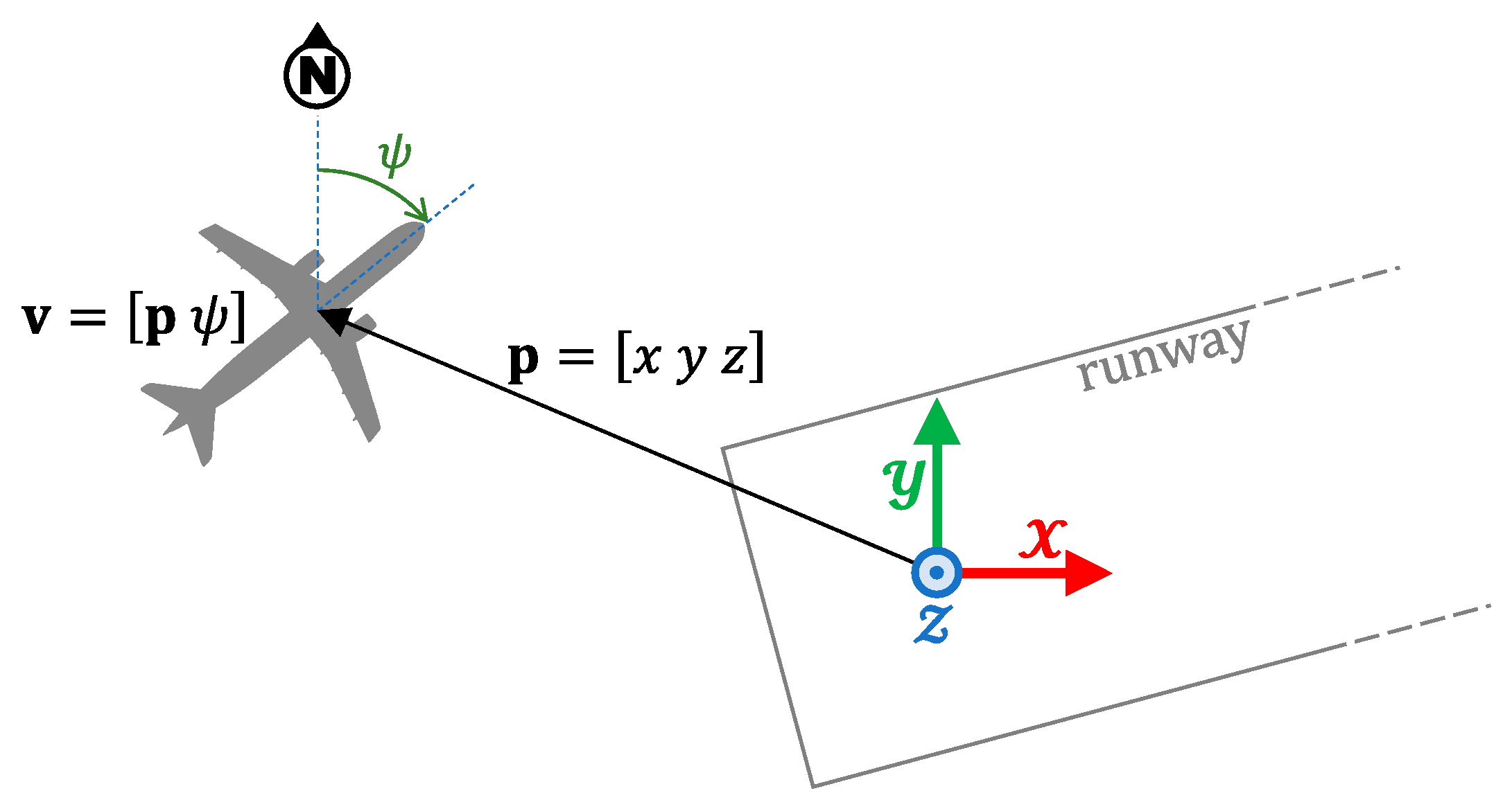
We assume that an approach procedure is completely defined by an ordered list or sequence of waypoints. Each waypoint consists of a tridimensional position and the required horizontal speed for the aircraft at this position. Formally, we define a tridimensional position as a vector $p=\left[xyz\right]$, where $x$, $y$, and $z$ (in $\mathrm{m}$) are given with respect to a coordinate system whose origin is located at the point of contact between the aircraft and the runway.

The position and heading of an aircraft at a given moment is expressed by the state vector $v=\left[p\psi \right]$, where $\psi$ is the angle between the North direction and the aircraft longitudinal axis (in $\mathrm{rad}$). Figure 1 illustrates the airspace model in the vicinity of a runway.

Let vector $u=\left[F_{\mathrm{s}}{V}_{\mathrm{s}}{Y}_{\mathrm{s}}\right]$ be the system input modeling the aircraft movement. The $F_{\mathrm{s}}$ and $V_{\mathrm{s}}$ parameters establish, respectively, the desired forward and vertical aircraft speeds (in $\mathrm{m}/\mathrm{s}$), and the $Y_{\mathrm{s}}$ parameter represents the angular speed of course change (yaw speed; in $\mathrm{rad}/\mathrm{s}$). In our model, the aircraft dynamics is defined by $\dot{v}=f\left(v,u\right)$ as

$$\{\begin{array}{c}\dot{x}=F_s\sin \psi \\ \dot{y}=F_s\cos \psi \\ \dot{z}=V_s\\ \dot{\psi }=Y_s\end{array}$$

(17)

3.2. Pilot’s Behavior

We formally define a waypoint as a vector $w=\left[ps\right]$, where $p$ establishes a tridimensional position and $s$ refers to the aircraft horizontal speed (in $\mathrm{m}/\mathrm{s}$). The algorithm presented in

Table 1. Pilot’s algorithm.

	$\mathbf{u}=\mathbf{pilot}\left(\mathbf{v},\mathbf{w}\right)$
1.	$\left[x_v{y}_v{z}_v\psi \right]=v$
2.	$\left[x_w{y}_w{z}_{w}s\right]=w$
3.	$F_{\mathrm{s}}=s$
4.	$\overline{vw}=\left[x_w-x_v,y_w-y_v\right]$
5.	$d_{xy}=\left|\overline{vw}\right|$
6.	$d_z=z_w-z_v$
7.	$V_s=\frac{d_z}{d_{xy}}{F}_s$
8.	$h=\left[\begin{array}{c}\sin \psi \\ \cos \psi \end{array}\right]$
9.	$Y_s=\mathrm{sgn}\left(\overline{vw}\cdot h\right)\frac{F_s}{r}$
10.	$u=\left[F_{\mathrm{s}}{V}_{\mathrm{s}}{Y}_{\mathrm{s}}\right]$

details the pilot’s behavior.

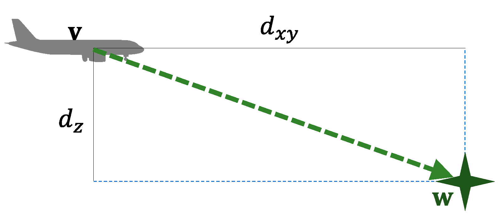
This establishes that the desired forward speed equals the waypoint speed. The desired vertical speed is computed according to the relation between vertical ($d_z$) and horizontal ($d_{xy}$) distances from the aircraft to the waypoint (see Figure 2).

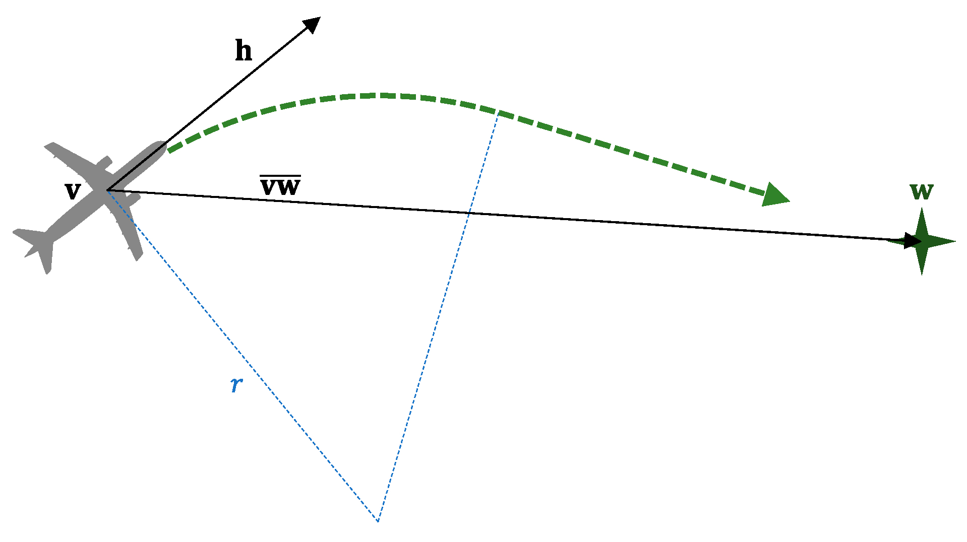
Additionally, the angular speed is computed to guarantee that the aircraft turns with a preestablished radius $r$ (see Figure 3). In this work, we assume a turn radius $r=1.52\mathrm{NM}$ ($2815\mathrm{m}$) [33].

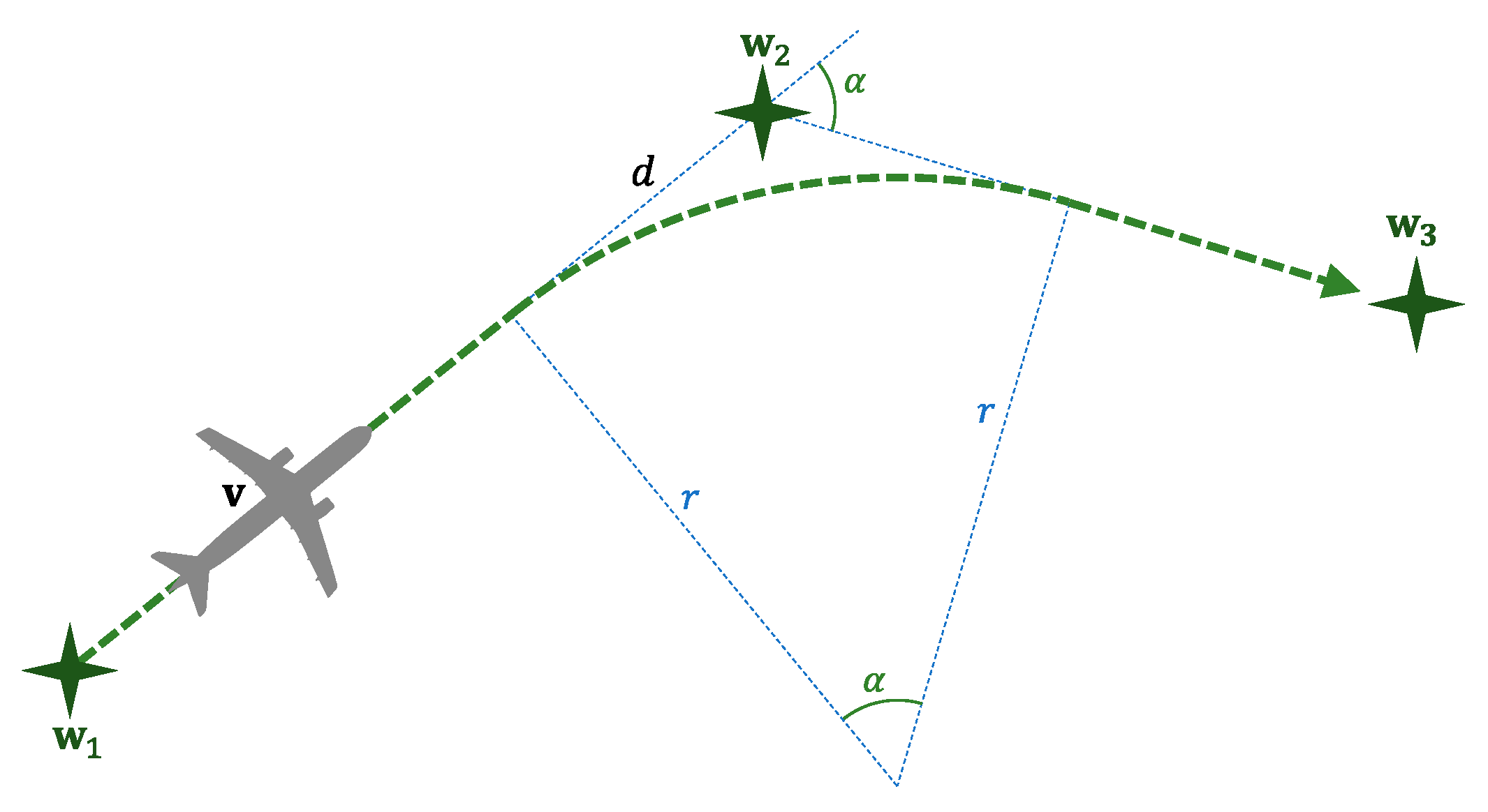
From the moment in which an aircraft enters the airport airspace, it must follow all the fly-by waypoints in the approach sequence. An aircraft should change to the next waypoint when it reaches the Distance-of-Turn Anticipation (DTA) to the current one. Figure 4 illustrates the geometry of this well-known problem. Let us assume that an aircraft located at $v$ is following the sequence of waypoints $\left\{w_1{w}_2{w}_3\right\}$. Assuming that the aircraft turns with a fix radius $r$, it should begin turning toward $w_3$ at a distance $d=r\tan \frac{\alpha }{2}$ from $w_2$.

3.3. Conflict Detection

We have considered an ideal conflict detector that continuously compares the position of all aircraft, analyzing if, at any time, two of them are closer than they can legally be. Specifically, as indicated, according to current regulations, the minimum allowable separation between two aircraft in the approach phase is $1000\mathrm{ft}$ vertically and $3\mathrm{NM}$ horizontally [2].

Table 2. Conflict detection algorithm.

	$\mathit{c}=\mathbf{conflict}\left({\mathbf{v}}_1,{\mathbf{v}}_2\right)$
1.	$\left[x_1{y}_1{z}_1~\right]=v_1$
2.	$\left[x_2{y}_2{z}_2~\right]=v_2$
3.	$d_{xy}=\left|\left[x_1{y}_1\right]-\left[x_2{y}_2\right]\right|$
4.	$d_z=\left|z_1-z_2\right|$
5.	if $z_1>29000ft$ then
6.	$\left[T_{xy}{T}_z\right]=\left[5\mathrm{NM}2000\mathrm{ft}\right]$
7.	else if $z_1>height\_th$ then
8.	$\left[T_{xy}{T}_z\right]=\left[3\mathrm{NM}1000\mathrm{ft}\right]$
9.	else
10.	$\left[T_{xy}{T}_z\right]=\left[0\mathrm{NM}0\mathrm{ft}\right]$
11.	end if
12.	if $d_z<T_z$ and $d_{xy}<T_{xy}$ then
13.	$c=true$
14.	else
15.	$c=false$
16.	end if

details a generic conflict detection algorithm. Symbol $~$ refers to the position in the state vector of the aircraft heading, which is not used by the algorithm. Parameter height_th refers to a height threshold below which checking is not carried out.

4. Conflict Prediction Based on Neural Network

As stated, the neural network that we propose to use as conflict predictor in this work is a binary classifier that, once trained, will be able to determine whether two approaching aircraft will break the separation rules during the maneuver. A database is required for the training of this neural network. The entries in this database must be labeled with the correct output that the network should provide in each case. As we must only differentiate between two classes (“conflict” or “not conflict”), two network outputs are possible in this case. To generate such a database, we need to focus on a specific airport (with an explicit approach maneuver), on which we will proceed to deploy a set of approaching aircraft by applying the aircraft and pilot models described in Section 3.1 and Section 3.2.

Next, we detail the scenario selected, the way in which the training database has been obtained, and the design and training process of our neural network.

4.1. Airport Scenario

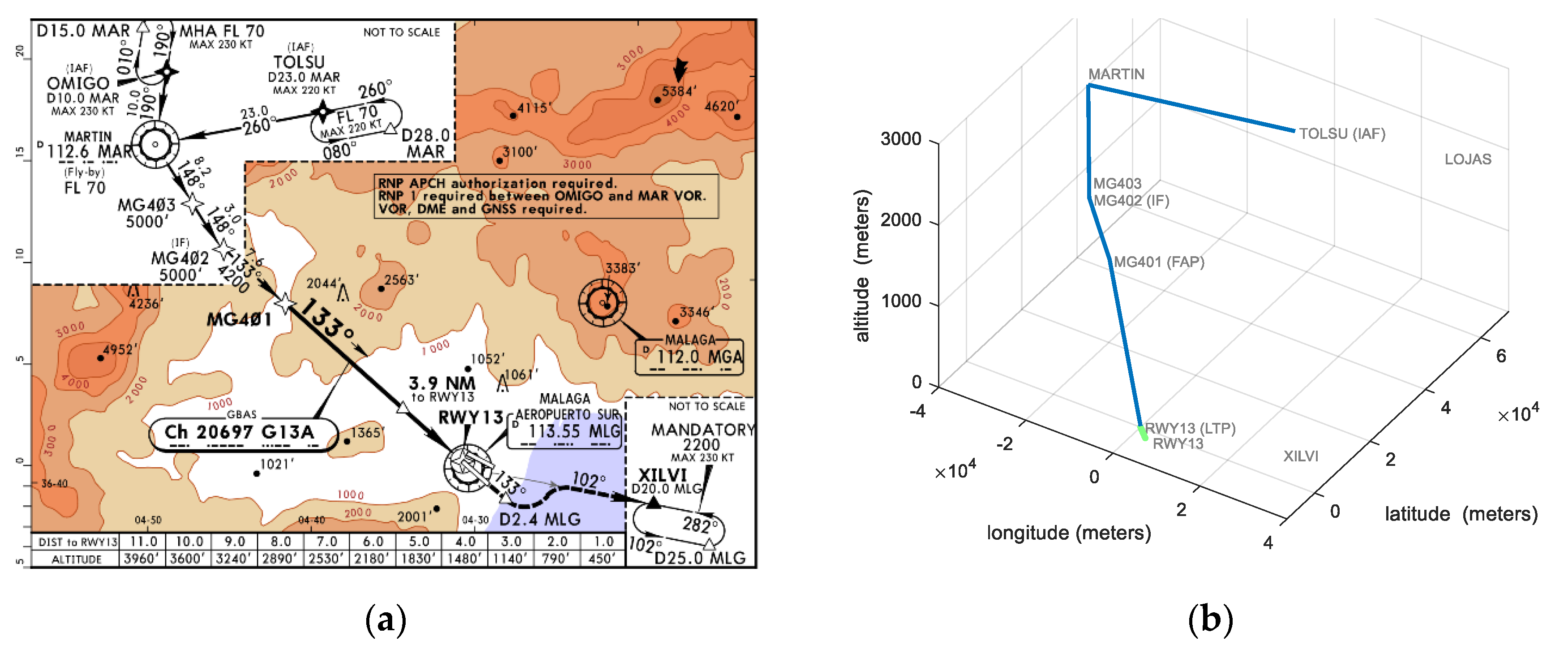
In our study, we have considered the approach procedure to the “RWY 13” runway of Málaga Airport (in Spain). Figure 5a shows part of the Instrument Approach Procedure (IAP) chart for this runway. Approach procedures are composed of several segments, referred to as initial, intermediate, and final approach segments, and a missed approach segment. These segments begin and end at designated fixes or specified points where no fixes are available.

During the initial segment, starting at the Initial Approach Fix (IAF), aircraft transit from an en-route airway to the intermediate segment. In our scenario, we assume that aircraft appear at LOJAS (see Figure 5b), and then they fly to TOLSU, as this is the IAF in this case. The next approach segment, which starts at the Intermediate Fix (IF), allows descent to an intermediate altitude and alignment of the aircraft to the runway. In the approach considered, the IF is MG 402.

Lastly, during the final approach segment, starting at the Final Approach Point (FAP), the aircraft navigates to the runway by using navigation aids, such as the Instrument Landing System (ILS) [11], which are located at or nearby the runway. The FAP in our scenario is MG 401. If the landing is successful, the maneuver is over. If, on the other hand, the pilot decides to perform a missed approach maneuver, then they must follow the instructions in the approach chart. In the case of Málaga, the chart indicates that aircraft must fly to XILVI in the case of missed approach.

Table 3. Detail of the approach procedure.

	Aeronautical Notation				Standard Notation
Waypoint Name	Latitude	Longitude	Height (ft)	Speed (kt)	X (m)	Y (m)	Z (m)	Speed (m/s)
LOJAS	37°12′26″ N	4°09′14″ W	7000	240	32,115.94	57,950.47	2133.60	123.47
TOLSU (IAF)	37°08′03″ N	4°28′15″ W	7000	240	3788.66	49,848.85	2133.60	123.47
MARTIN	37°03′19″ N	4°56′23″ W	7000	240	−38,123.21	41,103.20	2133.60	123.47
MG 403	36°56′23″ N	4°50′47″ W	5000	240	−29,788.86	28,279.77	1524	123.47
MG 402 (IF)	36°53′52″ N	4°48′45″ W	5000	160	−26,759.25	23,616.67	1524	82.31
MG 401 (FAP)	36°48′50″ N	4°41′39″ W	4200	160	−16,175.05	14,299.41	1280.16	82.31
RWY 13 (LTP)	36°41′04″ N	4°30′45″ W	52	140	55.74	−53.08	15.85	72.02
RWY 13	36°40′00″ N	4°29′20″ W	52	50	2179.44	−2035.92	15.85	25.72
XILVI	36°36′52″ N	4°06′01″ W	2200	220	36,907.56	−7831.11	670.56	113.18

details the complete sequence of waypoints defining this approach procedure, in both aeronautical and standard (SI) notation. As stated in Section 3.1, each waypoint consists of a tridimensional position and the required horizontal speed for the aircraft at this position.

4.2. Training Database

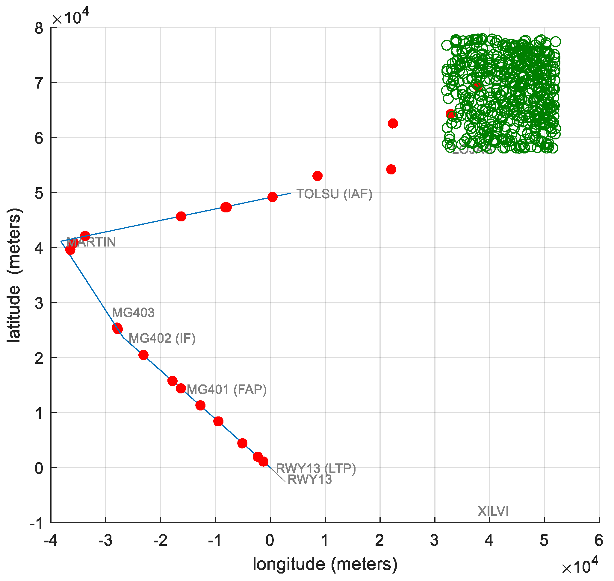
The training database has been obtained by using an airspace simulation tool developed in Matlab/Simulink [34]. This tool models, in a realistic way, the air traffic flow that approaches an airport runway. Figure 6 shows a snapshot of the graphical output provided by the simulator. As just detailed, the scenario considered in this work is one of the runways in Málaga Airport, and the aircraft dynamics modeled corresponds to the popular Airbus 320.

Instead of assuming that all aircraft are approaching from the LOJAS waypoint, we expanded the entry margin to a three-dimensional area of $20\mathrm{km}\times 20\mathrm{km}\times 500\mathrm{m}$. Aircraft will enter the airport airspace evenly distributed over that area. According to ICAO sequencing standards [2], we assume that a new aircraft appears every $60\mathrm{s}$. In Figure 6, the green dots represent the initial detection position for $1000$ aircraft, allowing this area to be visually delimited. On the other hand, each red dot represents an aircraft executing the approach maneuver. We assume that all arriving aircraft complete the maneuver.

If, at any given time during the simulation, there is a conflict between two flying aircraft (according to the criterion described in Section 3.3), the tool stores in the training database the positions in which both aircraft were first detected in airspace, as well as the difference in time between their apparitions. This entry is then labeled as conflict generator. If, on the other hand, an aircraft manages to land without conflicting with any other aircraft in airspace, then it can be paired with any of them, adding a new entry to the database (including similarly their respective initial positions and time difference) that will be labeled as not generating conflict.

For a neural network to train properly, it is necessary for the database to be balanced, that is, to contain approximately the same number of results of each of the elements that we want it to be able to predict in its output (i.e., output classes). In our case, the neural network will predict whether there is a conflict ($1$) or no ($0$) between a given pair of aircraft. As, in each simulation, there is a higher proportion of aircraft that are not in illegal positions than aircraft that actually are, only a third of the legal pairs of aircraft have been included to balance the database.

A training database should reflect all possible options that we may present in a neural network query. This is often a laborious task that results in databases with hundreds of thousands or millions of entries. In our case, we have generated a training database with half a million entries, structured as shown in

Table 4. Training database structure.

	Training Set		Validation Set		Test Set		Total Entries
Conflict TRUE	189,881	37.62%	23,735	4.70%	23,735	4.70%	237,351	47.03%
Conflict FALSE	213,863	42.38%	26,733	5.30%	26,733	5.30%	267,329	52.97%
Dataset	403,744	80.00%	50,468	10.00%	50,468	10.00%	504,680	100.00%

. As it can be seen, approximately half of the entries represent conflict situations. On the other hand, a training database is usually broken down into three separate parts. The first one is the set of entries dedicated to the training itself. The second part is the set of inputs used to validate the neural network design decisions. The last part is the set of inputs intended to evaluate the reliability of the resulting network. We have considered training, validation, and test sets of $80\%$, $10\%$, and $10\%$, respectively.

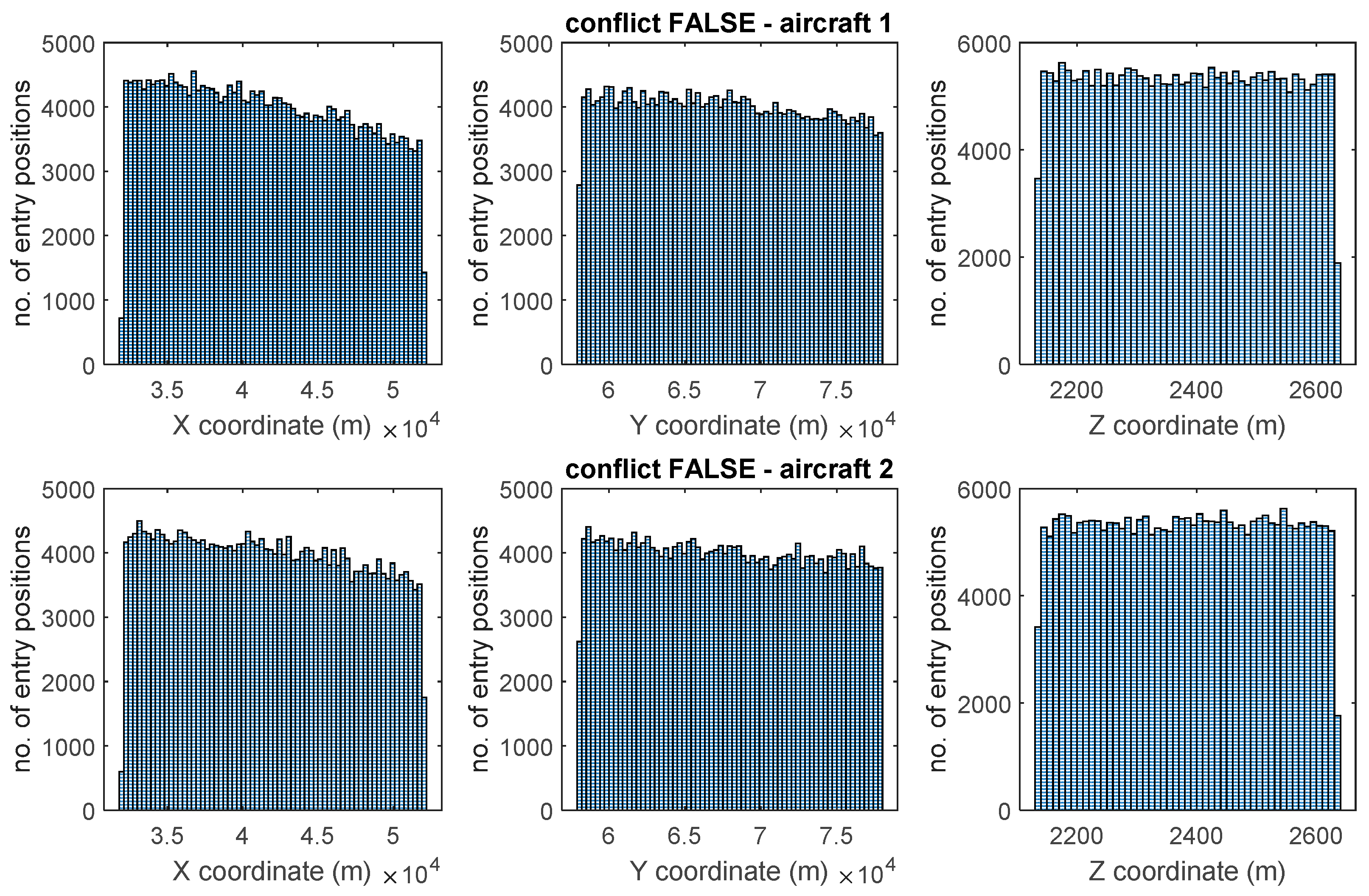
Next, we analyze the distribution of aircraft entry positions in the Málaga Airport airspace. We will look at the $504,680$ entries in Table 4 separately, depending on whether they caused a conflict or not. Figure 7 shows the initial spatial distribution of the $267,329$ analyzed aircraft pairs that turned out not to conflict (see Table 4). The figure contains two rows, showing the data for each of the aircraft involved. For each aircraft, the columns indicate its initial XYZ position. The six plots in the figure are histograms, that is, the horizontal axis is divided into fixed-width intervals, while the vertical axis shows the number of analyzed occurrences that fall into each interval. For example, we can see that, in almost $2000$ aircraft pairs, the initial height of aircraft 1 is between $2640$ and $2650$ m.

As indicated, to generate such initial positions, we have used a uniform random distribution within the established space, so it is to be expected that the histograms obtained will look relatively flat. We can see how the database inputs corresponding to pairs of nonconflicting locations generate flat-looking histograms in the XYZ coordinates.

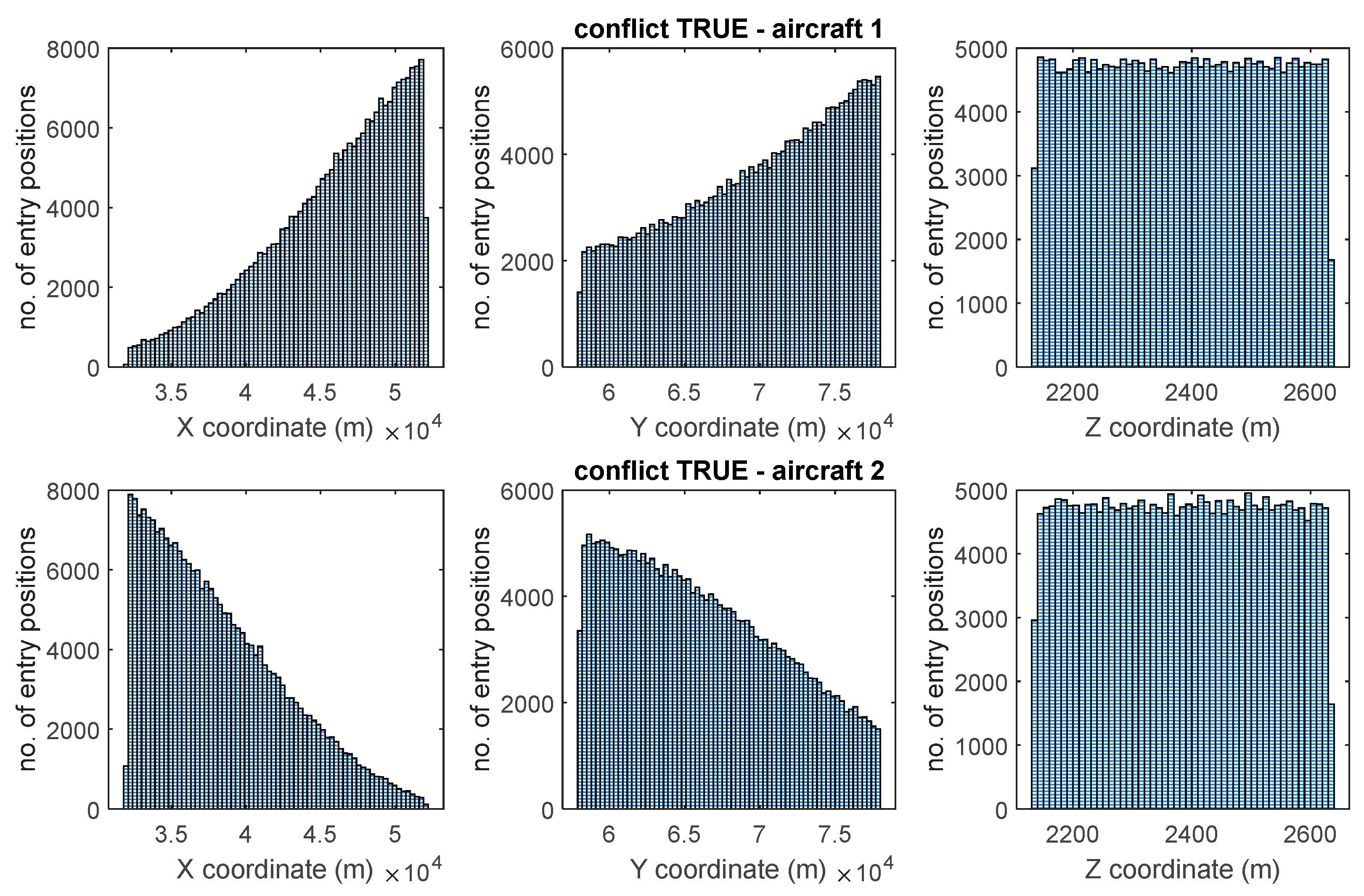
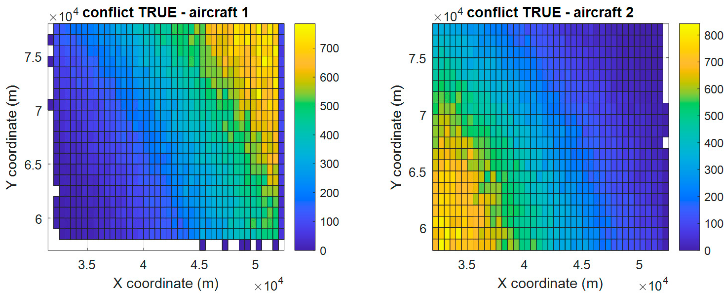
Figure 8 below shows the initial spatial distribution of the $237,351$ analyzed aircraft pairs that did come into conflict during their landing maneuver (see Table 4). The structure of this figure is similar to that of Figure 7 described previously. On this occasion, we can see that both the X and Y histograms have a clearly linear distribution, which indicates that the initial position in the plane has an effect on the generation of the conflict (as expected). By contrast, the Z histogram remains uniformly distributed, indicating that height does not affect the probability of conflict.

Figure 9 shows the same data as Figure 8, but in a way that makes it easier to explain the observed linear behavior. First, we discard the Z component (as it is kept uniformly distributed). Then, for each aircraft, we merge the X and Y histograms (both two-dimensional) into a single three-dimensional histogram, in which two dimensions are taken from the plane, and the third dimension is provided by a colored scale with the accumulated occurrences.

When an aircraft appears in the detection area, it heads toward the TOLSU waypoint, which is located to the southwest. Aircraft that are detected in the northeast are, therefore, more likely to conflict with subsequently detected aircraft and constitute section “aircraft 1” of a database entry. By contrast, aircraft that are detected in the southwest zone are more likely to conflict with previously detected aircraft, becoming the “aircraft 2” section of a database entry. This circumstance explains why the first aircraft presents a proportional distribution in the XY components, while the second aircraft has an inversely proportional distribution in those components.

4.3. Neural Network Design and Training

We have designed and trained our neural network employing the Matlab Deep Learning Toolbox [35]. This tool provides the user with several interfaces to visualize the state of the network and its progress in real time. The creation tool is also a graphical interface in which the different kind of layers can be dragged as blocks, building a graph that forms a very visual representation of the design of the network. It also offers the possibility of designing, creating, and training these networks through Matlab scripting, offering a flexibility comparable to Google’s popular TensorFlow framework [36].

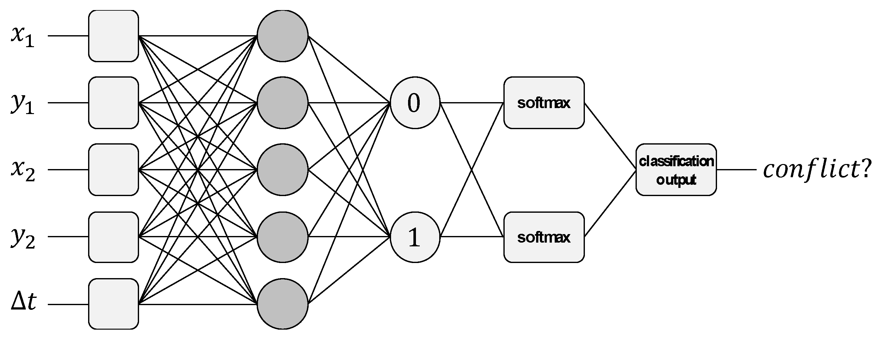
The design and training phases of a neural network are performed sequentially and iteratively, so that a design is trained, and its result helps in refining the original design. After training a huge number of networks, by varying the number of internal layers between $1$ and $8$, and the number of neurons per layer between $5$ and $64$, we have concluded that the problem can be solved by using the minimum MLP network shown in Figure 10.

In this design, Layer 1 contains five neurons whose function is to host the elements of the input vector ${\left[x_1{y}_1{x}_2{y}_2\Delta t\right]}^{⊺}$. Layer 2 acts as the inner hidden layer. It is fully connected, so that each neuron has five inputs and two outputs. Layer 3 is the output layer. It contains two neurons (with five inputs and two outputs) representing the possible responses provided by the network. If neuron $0$ is activated, the network will indicate no conflict. Conversely, if neuron $1$ is activated, the network will indicate the presence of conflict. Layer 4 performs a post-processing of the output. In particular, the softmax() activation function increases the differences between the possibility of getting a zero or a one [37]. Finally, Layer 5 incorporates a classifier that chooses which of the two options is most likely.

Regarding the learning function, we have considered three variants of SGD (see Section 2) provided by the Matlab Deep Learning Toolbox. The variants are Stochastic Gradient Descent with Momentum (SGDM) [32], Root Mean Square Propagation (RMSprop) [38], and Adaptive Moment Estimation (Adam) [39], the last one being finally chosen, as it offered the best accuracy in the experiments carried out.

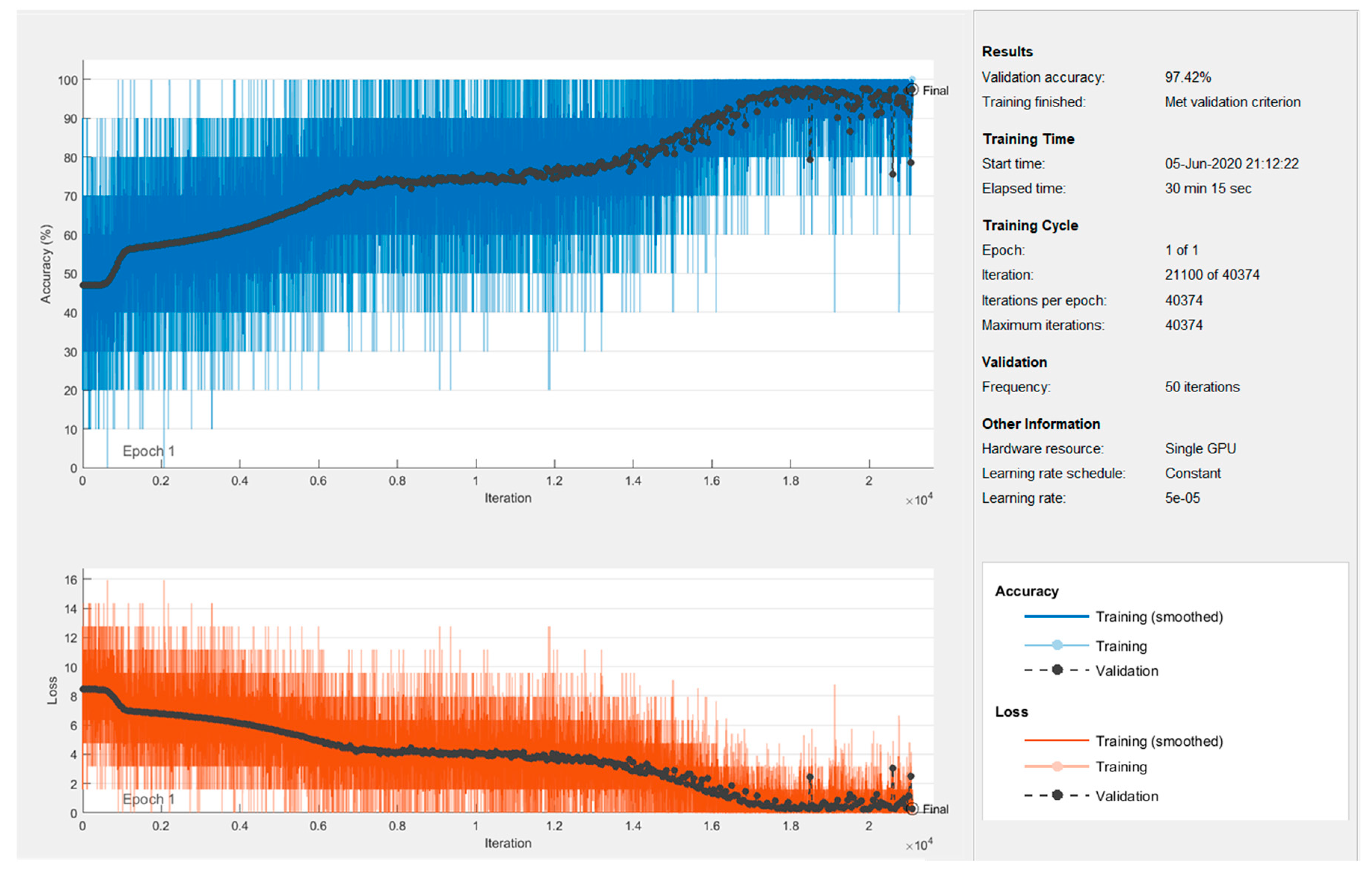
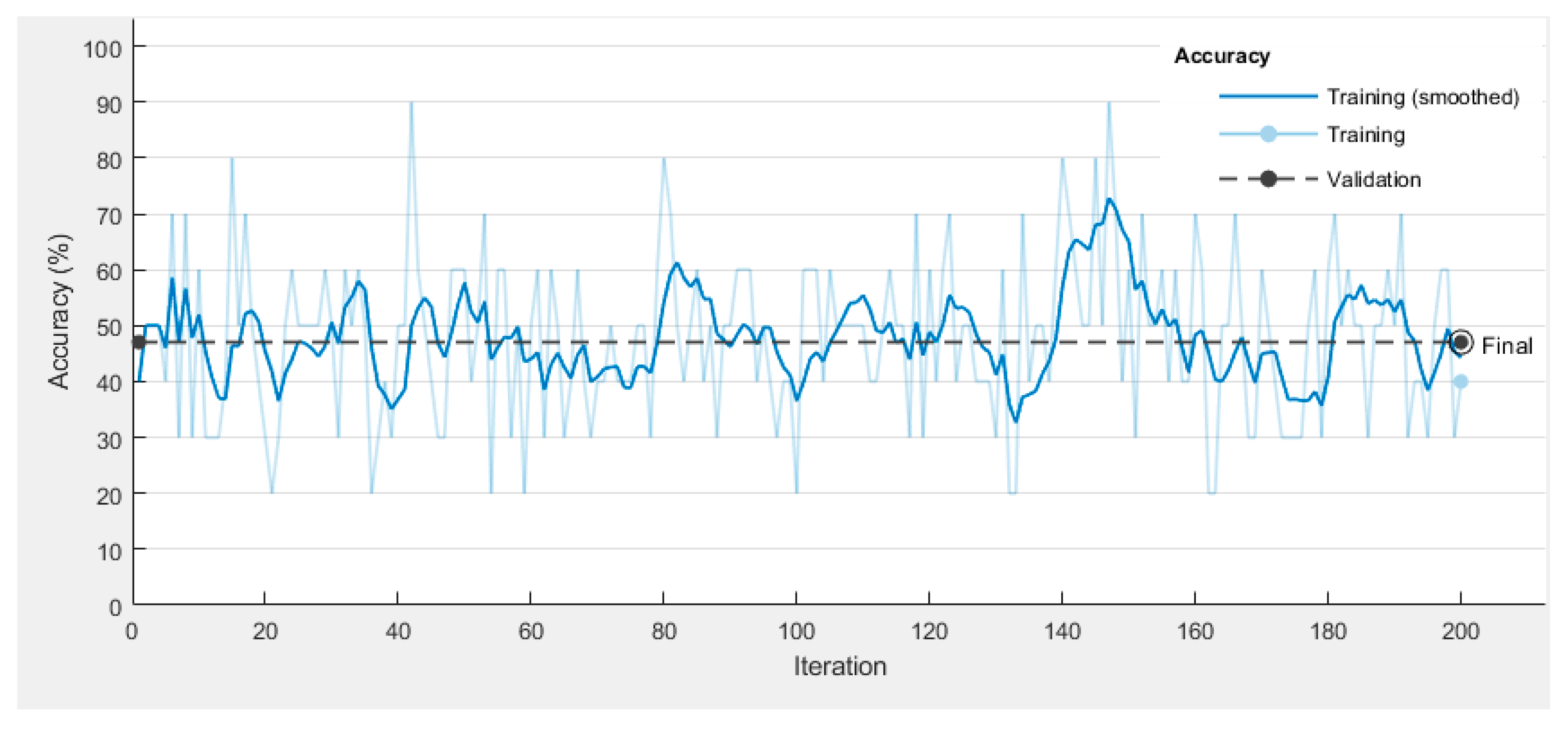
The neural network training process has been performed on a computer based on a ninth-generation Intel Core i9-9900K 3.6 GHz processor. Figure 11 shows its evolution. The upper part of the figure shows the network accuracy, while the lower part shows the loss. A batch size of $10$ entries has been applied. This means that the network is fed with a set of $10$ database entries, and then the adjustment of the neuron weights is performed according to the backpropagation algorithm detailed in Section 2. Therefore, the $403,744$ entries in the training set (see Table 4) lead to $40,374$ learning iterations. To avoid drastic fluctuations, the learning rate has been reduced to $5\times {10}^{-5}$. However, the scale of the figure is so large that it does not allow such an evolution to be observed. Figure 12 shows a very short training process, which allows us to better appreciate the behavior of the accuracy for successive iterations.

Every $50$ adjustment iterations, the accuracy of the network is checked against the $50,468$ entries in the validation set. This value (shown in black in the plots) is the one that really tells us if the network is learning properly. The training process has been configured to end after obtaining no improvement in $25$ consecutive validations. From here, it makes no sense to continue the process by submitting the network to an overtraining in which, far from improving, there is a worsening of learning. Finally, the trained network is able to correctly interpret $97.42\%$ of the validation vector. At this point, the accuracy obtained after presenting to the network the $50,468$ entries in the test set is $97.476$%.

To conclude our study,

Table 5. Trained neural network.

	Neuron	${\mathit{w}}_1$	${\mathit{w}}_2$	${\mathit{w}}_3$	${\mathit{w}}_4$	${\mathit{w}}_5$	$\mathit{b}\mathit{i}\mathit{a}\mathit{s}$
Layer 2	1	0.2880	−0.4528	0.1627	0.4580	−0.2579	0.0730
	2	−0.5185	0.4227	−0.2851	0.4557	0.5900	−0.0624
	3	0.6004	0.5419	0.5054	−0.7232	−0.3032	−0.0663
	4	−0.0130	0.3251	0.0855	0.2882	0.5579	−0.0674
	5	0.3818	0.7761	0.3995	−0.4928	−0.8459	0.0723
Layer 3	1	−0.4830	0.3597	−0.4186	0.0510	−0.1376	−0.0702
	2	−0.2686	0.4050	−0.9013	−0.4604	0.5170	0.0702

details the internal structure of the network resulting from the previous training. The table includes the weights for the five inputs of each neuron, as well as the bias applied to their output, for the fully connected layers $2$ and $3$.

5. Conclusions and Future Work

This work aims to verify the feasibility of using neural networks to implement an air traffic management support system to predict the occurrence of conflicts between aircraft in the approach phase. A possible implementation for this conflict predictor, based on a relatively simple multi-layer perceptron architecture, has been detailed. The high accuracy of the prediction (above 97%) allows us to conclude that neural networks may be the basis for a support system for the air traffic controller or the aircraft pilot, as it does not intend to replace them, but to provide them with critical information for decision-making. Applying the methodology detailed in this paper, the proposed conflict prediction tool can be easily deployed for any airport, either at the control tower or as an airborne system (without ground support), after training the neural network with historical data on approaches at that airport. As future work, we plan to improve different air traffic management operations in terminal maneuvering areas, focusing not only on arrivals, but also on departures. We also want to explore the possibility of extending the current study to the rest of the flight phases.

References

- ICAO. Traffic Growth and Airline Profitability Were Highlights of Air Transport in 2016. 2017. Available online: http://www.icao.int/Newsroom/Pages/traffic-growth-and-airline-profitability-were-highlights-of-air-transport-in-2016.aspx (accessed on 1 October 2020).
- ICAO. Doc 4444–PANS-ATM, Procedures for Air Navigation Services—Air Traffic Management; ICAO: Montreal, QC, Canada, 2016. [Google Scholar]
- Tang, J. Conflict Detection and Resolution for Civil Aviation: A literature survey. IEEE Aerosp. Electron. Syst. Mag. 2019, 34, 20–35. [Google Scholar] [CrossRef]
- Kuchar, J.K.; Yang, L.C. A Review of Conflict Detection and Resolution Modeling Methods. IEEE Trans. Intell. Transp. Syst. 2000, 1, 179–189. [Google Scholar] [CrossRef] [Green Version]
- Geser, A.; Muñoz, C. A geometric approach to strategic conflict detection and resolution. In Proceedings of the AIAA/IEEE Digital Avionics Systems Conference-Proceedings, Irvine, CA, USA, 27–31 October 2002; Volume 1. [Google Scholar] [CrossRef]
- Niu, H.; Ma, C.; Han, P.; Lv, J. An airborne approach for conflict detection and resolution applied to civil aviation aircraft based on ORCA. In Proceedings of the 2019 IEEE 8th Joint International Information Technology and Artificial Intelligence Conference, ITAIC 2019, Chongqing, China, 24–26 May 2019; pp. 686–690. [Google Scholar] [CrossRef]
- Chiang, Y.J.; Klosowski, J.T.; Lee, C.; Mitchell, J.S.B. Geometric algorithms for conflict detection/resolution in air traffic management. In Proceedings of the IEEE Conference on Decision and Control, San Diego, CA, USA, 12 December 1997; Volume 2, pp. 1835–1840. [Google Scholar] [CrossRef] [Green Version]
- Prandini, M.; Hu, J.; Lygeros, J.; Sastry, S. A probabilistic approach to aircraft conflict detection. IEEE Trans. Intell. Transp. Syst. 2000, 1, 199–220. [Google Scholar] [CrossRef]
- Liu, W.; Hwang, I. Probabilistic Trajectory Prediction and Conflict Detection for Air Traffic Control. J. Guid. Control. Dyn. 2011, 34, 1779–1789. [Google Scholar] [CrossRef]
- Yang, Y.; Zhang, J.; Cai, K.-Q.; Prandini, M. Multi-aircraft Conflict Detection and Resolution Based on Probabilistic Reach Sets. IEEE Trans. Control. Syst. Technol. 2017, 25, 309–316. [Google Scholar] [CrossRef] [Green Version]
- Moir, I.; Seabridge, A.; Jukes, M. Civil Avionics Systems; John Wiley & Sons, Ltd.: Chichester, UK, 2013. [Google Scholar]
- Beasley, J.; Howells, H.; Sonander, J. Improving short-term conflict alert via tabu search. J. Oper. Res. Soc. 2002, 53, 593–602. [Google Scholar] [CrossRef]
- Tang, J. Review: Analysis and Improvement of Traffic Alert and Collision Avoidance System. IEEE Access 2017, 5, 21419–21429. [Google Scholar] [CrossRef]
- Chaloulos, G.; Roussos, G.P.; Lygeros, J.; Kyriakopoulos, K.J. Mid and short term conflict resolution in autonomous aircraft operations. In Proceedings of the 8th Innovative Research Workshop and Exhibition, Proceedings, Brétigny-sur-Orge, France, 1–3 December 2009; pp. 221–226. [Google Scholar]
- Schmidhuber, J. Deep learning in neural networks: An overview. Neural Netw. 2015, 61, 85–117. [Google Scholar] [CrossRef] [PubMed] [Green Version]
- FAA. Instrument Procedures Handbook (IPH). 2017. Available online: https://www.faa.gov/regulations_policies/handbooks_manuals/aviation/instrument_procedures_handbook/ (accessed on 1 October 2020).
- Boeing. Statistical Summary of Commercial Jet Airplane Accidents Worldwide Operations | 1959–2018. 2019. Available online: https://www.boeing.com/resources/boeingdotcom/company/about_bca/pdf/statsum.pdf (accessed on 1 October 2020).
- Chen, M.Q. Flight conflict detection and resolution based on neural network. In Proceedings of the Proceedings—2011 International Conference on Computational and Information Sciences, ICCIS 2011, Chengdu, China, 21–23 October 2011; pp. 860–862. [Google Scholar] [CrossRef]
- Kaidi, R.; Lazaar, M.; Ettaouil, M. Neural network apply to predict aircraft trajectory for conflict resolution. In Proceedings of the 2014 9th International Conference on Intelligent Systems: Theories and Applications (SITA-14), Rabat, Morocco, 7–8 May 2014. [Google Scholar] [CrossRef]
- Le Fablec, Y.; Alliot, J.M. Using Neural Networks to predict aircraft trajectories. In In Proceedings of the International Conference on Artificial Intelligence, Las Vegas, NA, USA, 28 June–1 July 1999; pp. 524–529. [Google Scholar]
- Wang, Z.; Liang, M.; Delahaye, D. Data-driven Conflict Detection Enhancement in 3D Airspace with Machine Learning. In Proceedings of the 2020 International Conference on Artificial Intelligence and Data Analytics for Air Transportation (AIDA-AT), Singapore, 3–4 February 2020; pp. 1–9. [Google Scholar] [CrossRef] [Green Version]
- Wu, Z.; Tian, S.; Ma, L. A 4D Trajectory Prediction Model Based on the BP Neural Network. J. Intell. Syst. 2019, 29, 1545–1557. [Google Scholar] [CrossRef]
- Zhao, Z.; Zeng, W.; Quan, Z.; Chen, M.; Yang, Z. Aircraft trajectory prediction using deep long short-term memory networks. In Proceedings of the CICTP 2019: Transportation in China—Connecting the World—Proceedings of the 19th COTA International Conference of Transportation Professionals, Nanjing, China, 6–8 July 2019; pp. 124–135. [Google Scholar] [CrossRef]
- Ma, L.; Tian, S. A Hybrid CNN-LSTM Model for Aircraft 4D Trajectory Prediction. IEEE Access 2020, 8, 134668–134680. [Google Scholar] [CrossRef]
- Durand, N.; Alliot, J.-M.; Médioni, F. Neural Nets Trained by Genetic Algorithms for Collision Avoidance. Appl. Intell. 2000, 13, 205–213. [Google Scholar] [CrossRef]
- Alam, S.; McPartland, M.; Barlow, M.; Lindsay, P.; Abbass, H.A.; Bossomaier, T.; Wiles, J. Chapter 2 Neural Evolution for Collision Detection & Resolution in a 2D Free Flight Environment. In Recent Advances in Artificial Life; World Scientific Pub. Co. Pte. Lt.: Singapore, 2005; pp. 13–28. [Google Scholar]
- Christodoulou, M.; Kontogeorgou, C. Collision Avoidance in Commercial Aircraft Free Flight via Neural Networks and Non-Linear Programming. Int. J. Neural Syst. 2008, 18, 371–387. [Google Scholar] [CrossRef] [PubMed]
- Pham, D.T.; Tran, N.P.; Alam, S.; Duong, V.; Delahaye, D. A Machine Learning Approach for Conflict Resolution in Dense Traffic Scenarios with Uncertainties; Thirteenth USA/Europe Air Traffic Management Research and Development Seminar: Vienne, Austria, 2019. [Google Scholar]
- McCulloch, W.S.; Pitts, W. A logical calculus of the ideas immanent in nervous activity. Bull. Math. Biol. 1943, 5, 115–133. [Google Scholar] [CrossRef]
- Werbos, P.J. Beyond Regression: New Tools for Prediction and Analysis in the Behavioral Sciences. Ph.D. Thesis, Harvard University, Cambridge, MA, USA, 1974. [Google Scholar]
- The MathWorks Inc. Matlab. Available online: https://www.mathworks.com (accessed on 1 October 2020).
- Murphy, K.P. Machine Learning: A Probabilistic Perspective; The MIT Press: Cambridge, MA, USA, 2012. [Google Scholar]
- ICAO. Required Navigation Performance Authorization Required (RNP AR) Procedure Design Manual; ICAO: Montreal, QC, Canada, 2016. [Google Scholar]
- The MathWorks Inc. “Simulink.”. Available online: https://www.mathworks.com/products/simulink.html (accessed on 1 October 2020).
- The MathWorks Inc. Deep Learning Toolbox. Available online: https://www.mathworks.com/products/deep-learning.html (accessed on 1 October 2020).
- Google. TensorFlow. Available online: https://www.tensorflow.org (accessed on 1 October 2020).
- Bishop, C.M. Pattern Recognition and Machine Learning; Springer: New York, NY, USA, 2006. [Google Scholar]
- Tijmen, T.; Hinton, G.; Lecture 6.5-rmsprop: Divide the gradient by a running average of its recent magnitude. COURSERA: Neural Networks for Machine Learning. 2012. Available online: https://www.cs.toronto.edu/~tijmen/csc321/slides/lecture_slides_lec6.pdf (accessed on 1 October 2020).
- Kingma, D.P.; Ba, J. Adam: A Method for Stochastic Optimization. arXiv 2014, arXiv:1412.6980. [Google Scholar]
Figure 1.
Airspace model.
Figure 2.
Vertical speed computation.
Figure 3.
Turn direction computation.
Figure 4.
Distance-of-Turn Anticipation (DTA) concept.
Figure 5.
Approach chart (a) and 3D view (b) of the approach path.
Figure 6.
A set of simulated aircraft approaching the Málaga Airport (upper view).
Figure 7.
Entry positions distribution of nonconflicting pairs of aircraft.
Figure 8.
Entry positions distribution of conflicting pairs of aircraft.
Figure 9.
XY distribution of conflicting aircraft entry positions.
Figure 10.
Neural network .
Figure 11.
Neural network training process.
Figure 12.
Example of accuracy evolution.