Fractional PIλD Controller Design for a Magnetic Levitation System


Department of Automatic Control and Robotics, AGH University of Science and Technology, Al. Mickiewicza 30, 30-059 Kraków, Poland
*
Author to whom correspondence should be addressed.
Electronics 2020, 9(12), 2135; https://0-doi-org.brum.beds.ac.uk/10.3390/electronics9122135
Submission received: 11 November 2020
/
Revised: 6 December 2020
/
Accepted: 9 December 2020
/
Published: 13 December 2020
(This article belongs to the Special Issue Fractional-Order Circuits & Systems Design and Applications)
Abstract
:Currently, there are no formalized methods for tuning non-integer order controllers. This is due to the fact that implementing these systems requires using an approximation of the non-integer order terms. The Oustaloup approximation method of the fractional derivative is intuitive and widely adopted in the design of fractional-order PID controllers. It requires special considerations for real-time implementations as it is prone to numerical instability. In this paper, for design and tuning of fractional regulators, we propose two methods.The first method relies on Nyquist stability criterion and stability margins. We base the second on parametric optimization via Simulated Annealing of multiple performance indicators. We illustrate our methods with a case study of the PID controller for the Magnetic Levitation System. We illustrate our methods’ efficiency with both simulations and experimental verification in both nominal and disturbed operation.
1. Introduction
The magnetic levitation system is a highly relevant area of control design. It is because these systems have many varied uses such as in minimal friction bearings, high-speed maglev passenger trains, levitation of wind tunnel models, vibration isolation of sensitive machinery, levitation of molten metal in induction furnaces, and the levitation of metal slabs during manufacture, see [1]. Research on this topic has led to the development of efficient magnetic bearings (see [2]) and flywheels for space satellite low earth orbits, hybrid electric vehicles (see [3]), and many stationary applications. An important direction of research in this area is also an active magnetic bearing, which was described in their works by among others—Srinivas (see [4]), Uzhegov (see [5]), and Kandil (see [6]).
A very important area of the research about the active magnetic levitation system is control structure. They are naturally unstable, so they require control. Many researchers considered this topic (see [1]) and Joo and Seo (see [7]) designed linearizing feedback control for the magnetic levitation system to PID controllers. The comparison of this approach with Takagi–Sugeno fuzzy control (see [8]). Baranowski and Piątek (see [9]) presented a cascade variant of the linearizing feedback. Bloch (see [10]) discussed real-time neural feed-forward control. Piątek (see [11]) designed and implemented quick linear control for active magnetic levitation systems based on FPGA circuits.
Research on the control of magnetic levitation using non-integer (fractional) systems was one of the first attempts by Piłat (see [12], where a non-integer order PD controller was considered. Tepljakov et al. (see [13,14]) described the problem of fractional-order PID controller design for a model of a magnetic levitation system. The latest research focuses on the digital implementation of non-integer controller for a real plant; this topic was considered by Chopade et al. [15], Rojas et al. [16] and Ananthababu et al. [17]. Pandey et al. (see [18,19]) proposed an anti-windup fractional PID controller for magnetic levitation. Roy et al. (see [20]) presented a comparative study between the Sliding Mode Controller and Fractional Order Sliding Mode Controller when applied to a magnetic levitation system. Swain et al. (see [21]) presented real-time implementation of fractional order PID controllers for a magnetic levitation.
Most of these results that are simulated based or experimental are hard to replicate or use not precisely for fractional approximations, which makes the fractional part debatable.
Contributions of this paper are:
- we propose two different methods of controller parameter selection for the active magnetic levitation system,
- and we provide experimental verification of both design methods.
This paper is organized as follows. Section 2 presents a brief introduction to the mathematical model of the magnetic levitation laboratory system. In the next section, the authors present a non-integer PID controller and proposed two methods of tuning these parameters. In Section 4, the authors show an example of using a proposed method for construction of a PID controller for the laboratory magnetic levitation system. The next section describes the implementation of the controller in real-time systems. The results of the experiments are described in Section 6.
2. The Mathematical Model of the Magnetic Levitation Laboratory System
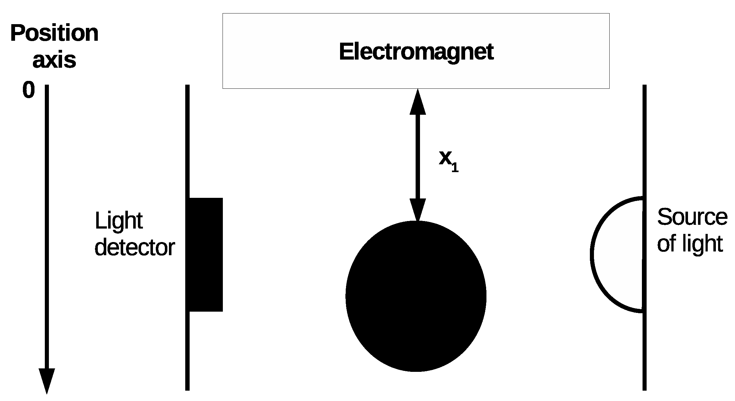
The magnetic levitation system (see Figure 1) consists of the electromagnet, the ferromagnetic sphere (which we will be calling ”ball”), the current driver, and the position measurement system consisting of the light source and the light sensor.
The mathematical description of the system will be based on Newton’s second law, where is the ball position, measured as the distance from the electromagnet, is the electromagnet coil current, and is the ball velocity. Ball speed can by calculated from value of force generated by the electromagnet, m is the mass of the ball, and g is the gravitational acceleration. The velocity of ball is given by formula (see [1,23]):
where a and b are positive constants. Parameters a and b were determined by analysis of a series of steady state points of the system with a closed stabilizing feedback loop. The exponential function was fitted into these points through a least squares minimization. For details, see [23].
The coil current in the system usually is influenced by many factors like changes in inductance, velocity, and others. However, our system includes a current driver, which has its own feedback loop. This solution is very popular (see [24]) because it leads to either lower order or simpler model structure. In an optimal situation, the driver should allow full current control; however, in real situations, it introduces its own dynamics. For the system considered, these dynamics can be sufficiently modeled by a first order dynamical system given by the following equation:
where is the control voltage, is the gain of current controller, is the time constant of the current driver, and is the zero error of current driver.
Let us introduce state space vector given by
which can be used to formulate the model of the system as the following system of first order differential equations:
All variables and parameters used in the model are described in Table 1. We use exponential approximation for the electromagnetic strength formula. A detailed discussion of such choice can be found in [25].
It is a known fact that the linear controller can operate properly in the neighborhood of a chosen steady state. Performance of classical PID can be strongly improved, if the appropriate reference control value corresponding to a reference value is added to the generated control signal. The authors tested this solution with different types of non-integer PID controllers, see [26,27,28]. The constant value added to the control signal we can calculate by formula:
where
and is the desired position of the ball.
The control loop of the described system was presented in Figure 2.
3. Method of Tuning of a Non-Integer Order PID Controller
One of the major tasks in the implementation’s field of the fractional PID controller is the formulation rules of tuning them. In this section, first we describe the concept of the PID controller with a fractional integrator, and then we propose two approaches of tuning it. The first one relies on introducing a fractional integral to a stabilizing PD controller and studying stability margins via the Nyquist criterion. The second one uses simulated annealing and multiple performance indicators. Both approaches are support methods requiring appropriate selection by the user.
3.1. Non-Integer PID Controller
Podlubny (see [29]) proposed a generalization of the PID controller, namely the PID controller, involving an integrator of order and a differentiator of order . As can be observed, when and , we obtain a classical PID controller, similar to when and give PD, and give P, and give PI. All these classical types of PID are the particular cases of the fractional PID. However, the PID is more flexible.
For laboratory active magnetic levitation systems, we used controllers by structured PID. In the time domain, the equation for this controller’s output has the form:
where is the Caputo derivative of order with respect to time, which is equivalent to the fractional integral of order , and:
- is proportional gain
- is integral gain
- is derivative gain
- is control deviation in time t
In addition, the transfer function formula is given by the equation:
3.2. Analytic Tuning Method with Nyquist Stability Criterion
This section describes the analytically procedure for determining the settings of the PID. They base the developed procedure on the Nyquist characteristic. The procedure of determining the PID controller settings can be performed by the following steps:
- Determine the system work point.
- If the system is nonlinear, calculate the linearized system of the work point.
- Determine the stability region for the integer part of the controller. For example, if you want to create a controller PID, you must calculate the stability region of a PI controller.
- Use a Nyquist criterion to determine the order of a non-integer order part of the regulator and this gain for a reasonable stability margin.
The advantage of this method is that we have an analytical description of the properties of the system—on the basis of which we can easily determine the stability area, gain, and phase margin. The most important disadvantage of this approach is that, for more complex systems, it can be difficult or not applicable.
3.3. Tuning by Simulated Annealing
Simulated annealing is a probabilistic technique for approximating the global optimum of a function. This algorithm uses a meta-heuristic to approximate global optimization in a large search space for an optimization problem—for problems where finding an approximate global optimum is more important than finding a precise local optimum in a fixed amount of time.
The advantage of this method is the ability to define any quality index for optimization, and there is no need to analytically determine the properties of the system. This method also allows the design of the regulator to bend known control characteristics. The disadvantage is the time needed to perform the optimization.
4. Design of the Controller for a Magnetic Levitation System
4.1. Construction PID for Magnetic Levitation Systems Using the Analytic Method
To perform the calculations and simulations, the following assumptions have been made:
- mm.
- Regulator must work for frequency bound between and Hz.
- Order of approximation use for implemented non-integer elements must have value 5.
Based on assumptions, we can determine the work point of the system as:
In the next step, we calculate the transfer function of the linearized system in the work point:
where have the form:
Then, we designed a classical PD controller which will stabilize the system. The stability region can by described by equation:
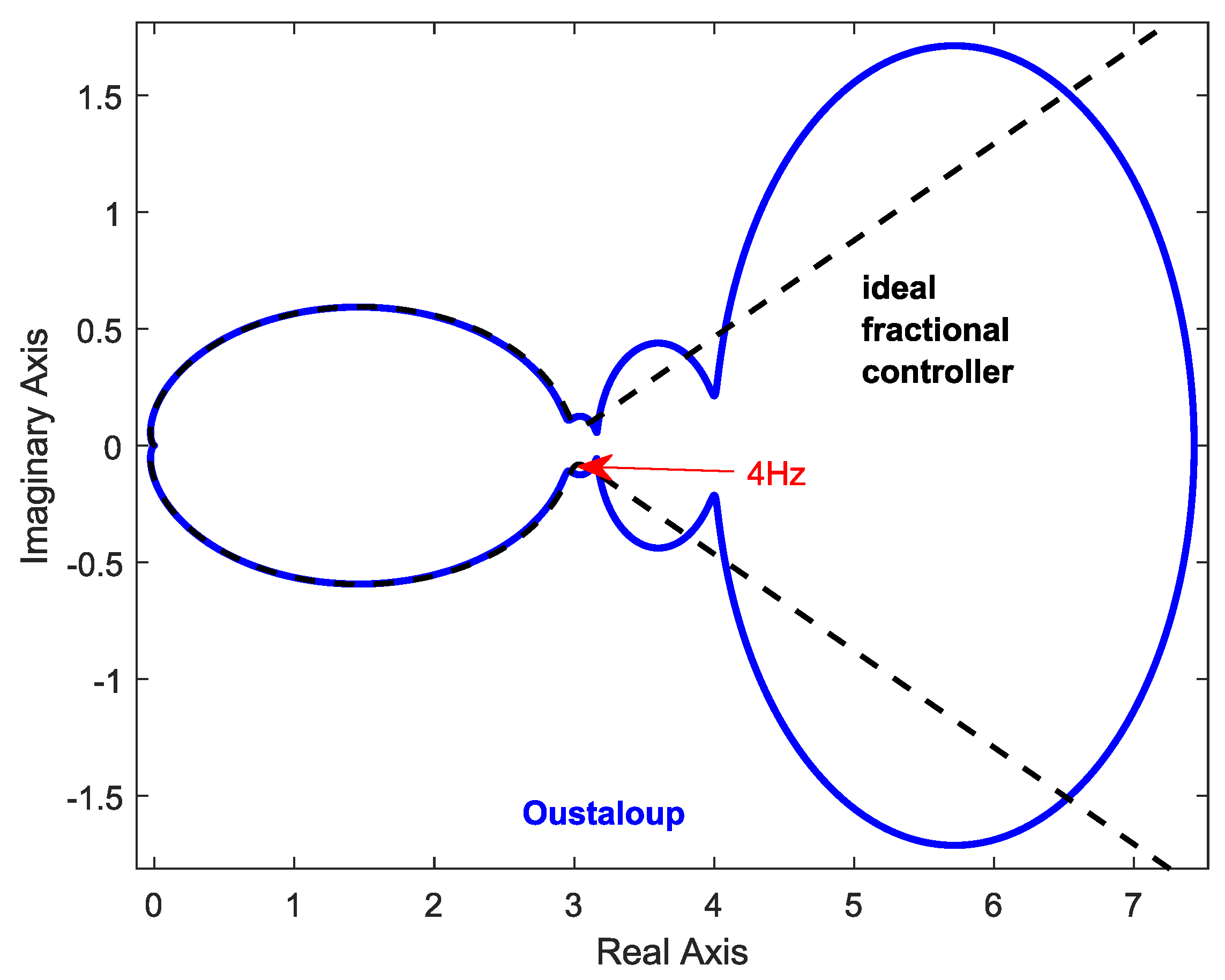
Finally, a stability analysis based on the Nyquist criterion was performed. The Nyquist plot of the designed ideal (non-approximated) non-integer controller is presented in Figure 3 with a dashed line. Fractional controller parameters for these systems have value: , , and . As we can see, these parameters fully meet the assumptions.
4.2. Tuning of PID Using Simulated Annealing
In this case, we can define the decision variables as: , , , . The tests will be conducted for the following quality indicator:
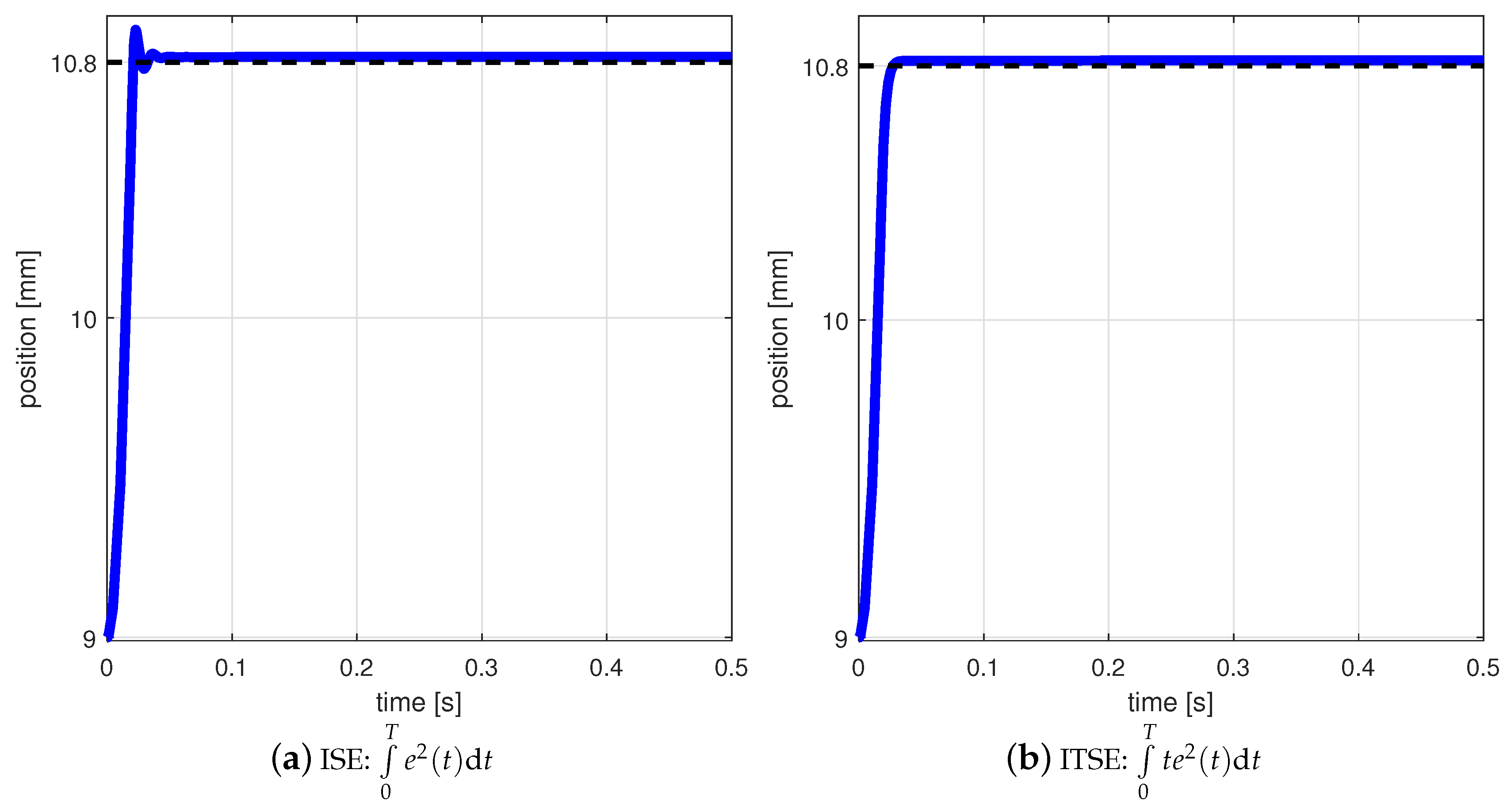
- ISE:
- ITSE:
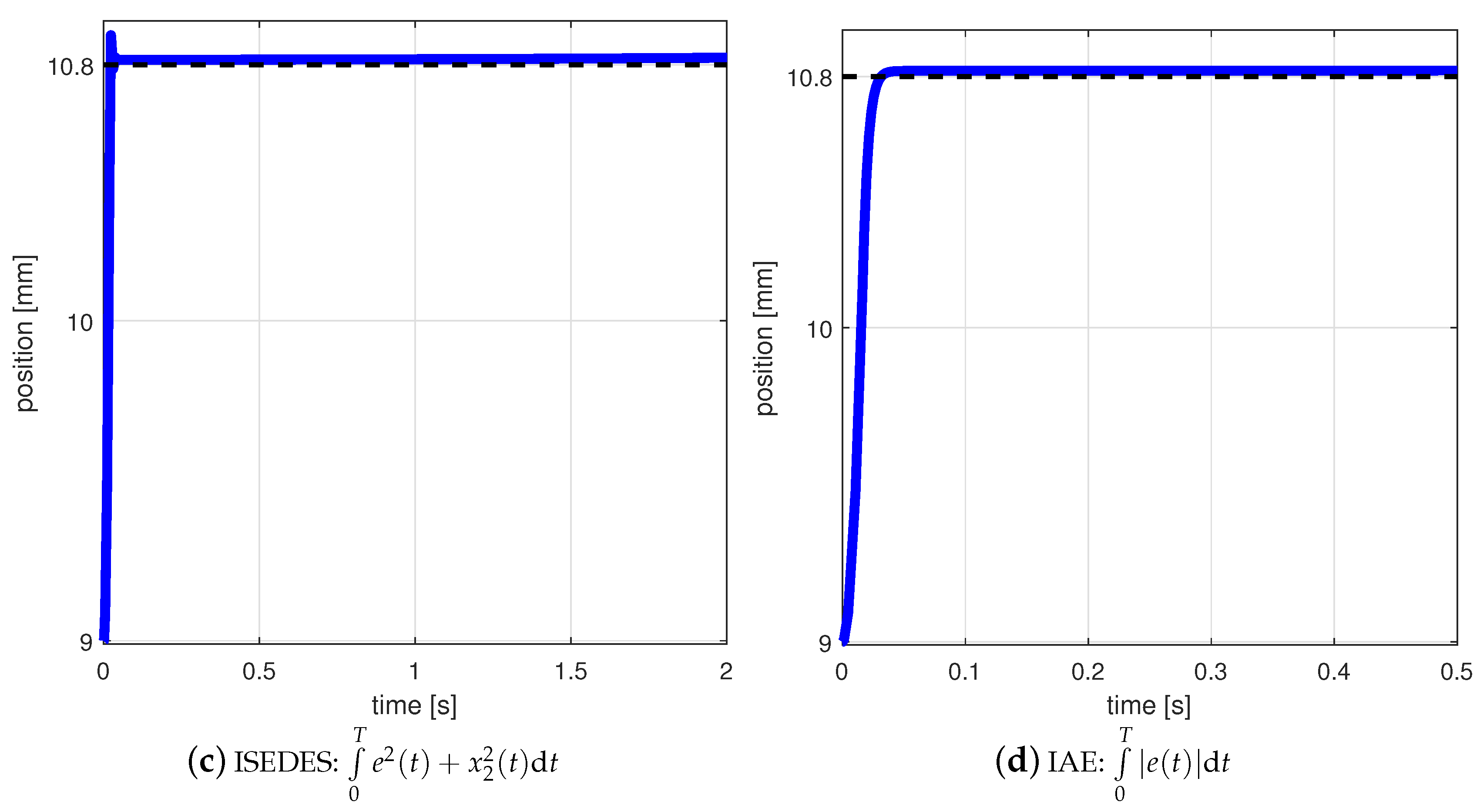
- ISEDES:
- IAE:
where . We use all of these qualities’ indicators because have different properties. ISE is one of the most used quality indicators. Since it is simple to use, it provides good results and in many cases can be calculated analytically. Its disadvantage is that it favors large errors, which means that, in the tuning process of the controller, errors at the beginning of the control process will have a greater impact on this process.
The ITSE quality indicator eliminates the problem of large fluctuations at the ends of the optimization horizon by multiplying the square of the control error by time. It is possible because the big value of errors at the beginning of the control process is leveled by multiplication by the small value of time; the same thing happens at the ending phase of the control process when the small value of errors are multiplied by the big value of time. This eliminates a significant influence of the error from the initial control phase on the value of the quality indicator.
ISEDES takes into account the rate of change of the error value, which allows for taking into account the dynamics in the optimization process. However, it has the same problems as quality indicator number 1.
IAE is presented, which treats all error values in the same way. However, its major disadvantage is that it can only be used in simulation environments because the analytical form of its solution does not exist. For more details, see [26,27,30,31].
Optimization start points have the following values:
Simulation initial value:
- —since the system is inherently unstable, the starting point must be around the setpoint.
- —the sphere has no initial velocity.
- —value determined by Formula (6).
The optimal PID settings for the system are collected in Table 2. Position states of the magnetic levitation were shown in Figure 4. When analyzing the charts, we see that in all cases the system stabilizes around the set value in less than s. In all cases, you can see that there is a slight fix error. In the case of quality indicators 1 and 2, there is also a noticeable overshoot in the initial phase of the control process of magnetic levitation.
It is also visible in the values of the quality indicators collected in Table 2. Note that, for the quality indicators 1 and 3, the values of the , , and parameters are similar. The highest values were also obtained for the indicators defined in this way. On the other hand, for the indicators defined with Formulas (2) and (4), the values of the and parameters are similar. Additionally, it should be mentioned that the value of is similar in all cases.
How can we see that the best result has been achieved when the quality indicator has form IAE? It should be noted that all quality indexes values are very close to each other. For this reason, the controller settings for the test in to laboratory system were selected values from IAE.
5. Realization Non-Integer Order PID Controller in a Real-Time Environment
5.1. Time Domain Oustaloup Approximation
The controller was implemented with the time domain Oustaloup method. This method was based on the classical Oustaloup approximation method, where fractional-order operator can be approximated by (see [32]):
where:
The proposed approach is to realize every block of the transfer function (16) in the form of a state space system. Those first order systems will then be collected in a single matrix resulting in full matrix realization. This continuous system of differential equations will then be discretized. The time domain approximation has formulas:
This can be written in vector matrix notation
or in brief
What can be immediately observed is that the matrix is lower triangular. This is an extremely important in the case of this problem, as all its eigenvalues (poles of transfer function (16) are on its diagonal, so there is no need for eigenvalue products, which would lead to rounding errors. This is why discretization of (21) should have a structure preserving property.
The implementation of the algorithm requires the discretization of the control system designed in a continuous time domain. For preserving the stability attributes of the system in the discrete time domain, as supposed, the Tustin method also known as the bilinear transform for triangular matrix, has been chosen (see [33]). For more details about performance of time domain Oustaloup and realization fractional systems in real-time systems, see [28,34,35,36,37].
5.2. SoftFrac
The SoftFrac package was used to implement the regulators. SoftFrac gives Matlab user functionality to create a state-space system and transfer function fractional model of the non-integer dynamic element based on approximations: Oustaloup (see [32]), time domain Oustaloup (see [38]), and LIRA (see [39]). The state-space fractional model class (ssf) inherits from standard state-space model class (ss) and have all of the functionality of this class, while the transfer function fractional model class (tsf) inherits from a transfer function model.
Because the SoftFrac library uses inheritance mechanism in implementation, the user can use all functionalities of parent classes ssf and tsf. In particular, the user can use this realization for Simulink simulation, system behavior analysis, and easy plotting of dynamic characteristics. In addition, we have added to the classes a construction method for easy conversion between those types, from ssf to tsf and vice versa.
6. Experiment Results
The controller performances for the magnetic levitation system has been investigated based on results from tuning methods in the following experiments:
- Introducing the ball into the magnetic field from below, near the working point by hand. Then, we waited for the ball’s position to stabilize at the working point.
- The experiment begins when the sphere is at the working point. It consists of knocking the sphere out of position by means of strokes.
The laboratory magnetic levitation system consists of: electromagnet, ferromagnetic sphere-position sensor, and current sensor power interface. The position measurement is done by the light source and sensor.
We can see in Figure 5 that the distance is measured from electromagnet to ball. The position measurement is based on the amount of light falling on the detector.
The composition of the laboratory stand on which the experiments were carried out included: PC, magnetic levitation plant (see [22]), and RT-DAC/PCI process board (see [40]) developed by INTECO. The computer on which the experiments were conducted used the Matlab 2015b version with the MATLAB/RT-CON real-time library installed. This computer used Windows 7 Professional, 64 GB RAM operating memory, and Intel Core I5 3.2 GHz.
RT-DAC/PCI I/O is a multifunction analog and digital I/O board dedicated to real-time data acquisition and control. The board contains a Xilinx FPGA chip. These boards can be reconfigured to introduce a new functionality of all inputs and outputs without any hardware modification. By default, the configuration version board accepts signals from systems and generates PWM outputs, and is equipped with the general purpose digital input/outputs (GPIO), A/D and D/A converters, timers, counters, frequency meters, and chronometers. The boards can be applied:
- using one of ready-to-use configurations distributed with the boards,
- using a new customer-specified configuration.
In this approach, the order of the non-integer order integrator approximation has been selected in the range with sampling time of second.
Experiments have been conducted to validate the robust properties of the designed controller. The discrete Oustaloup approximation has been implemented in a real-time environment with the use of a RT-DAC process board and a MATLAB/RT-CON real-time library.
6.1. Analytic Method
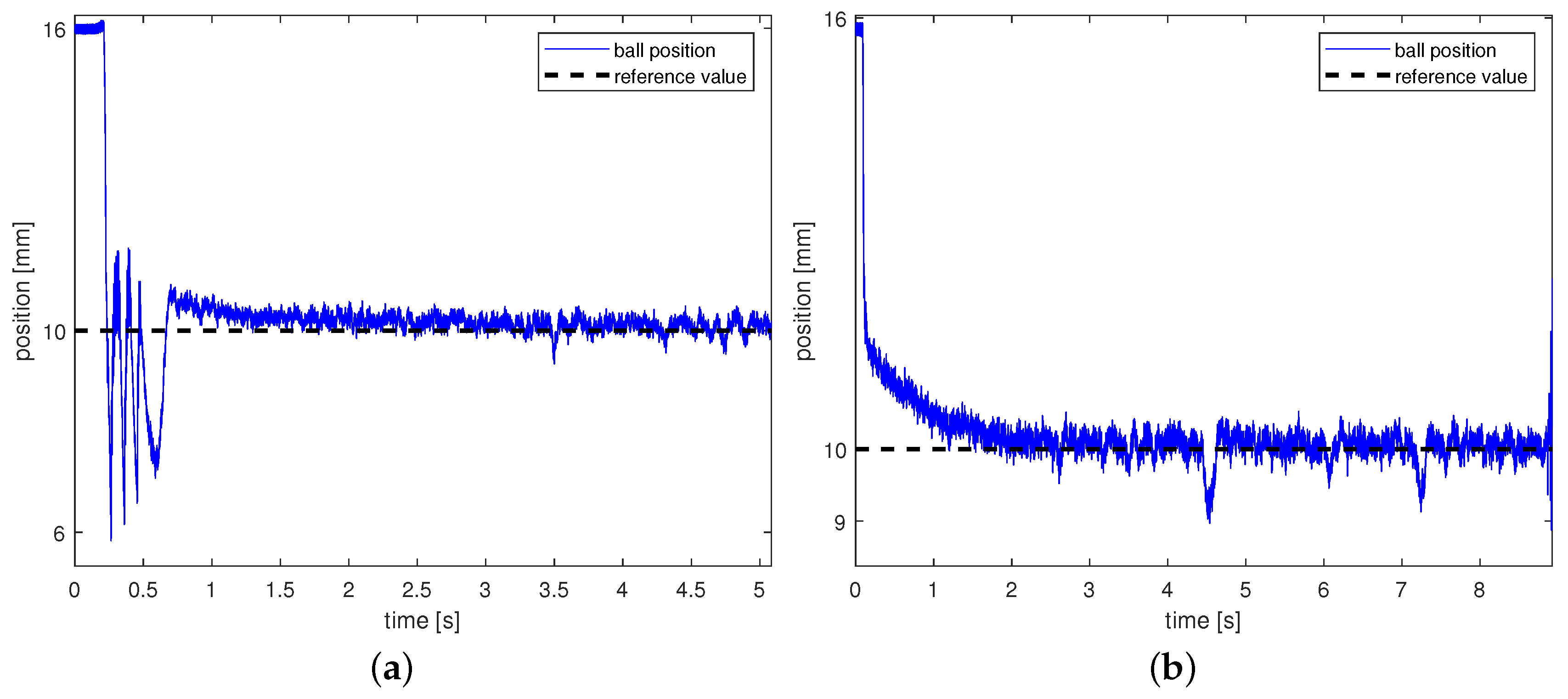
In Figure 6a, one can find the stabilization position process in point 10mm. As can be seen, PID controller stabilizes the system position in s.
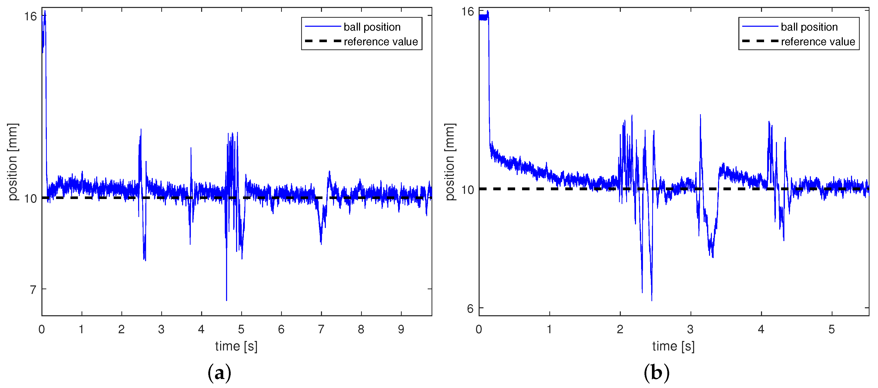
The second experiment, presented in Figure 7a, shows the disturbance rejection for the controller. The system has been disrupted at about 2.5 s, 3.7 s, and 5.0 s.
6.2. Results of Tuning by Simulated Annealing
In Figure 6b, we see the stabilization position process for a regulator with settings from the tuning process. As can be seen, this controller needs more time to stabilize the system position, about 8 s.
The second experiment, presented in Figure 7a, shows the disturbance rejection for the controller. The system has been disrupted at about 2.5 s, 5 s, and 7 s. It should be noted that the regulators in both cases cancel the disturbance very well. This shows the high level of robustness of the regulators.
7. Conclusions
Control design for the magnetic levitation system, while known, is still useful as a benchmark for both control quality and implementation purposes. The main issue that is known with fractional controllers is the problem of infinite memory. Direct implementation of fractional integrals (or derivatives) require either the summation of a series of signal samples with increasing length and varying coefficients or computing convolution integrals with singular kernels on expanding intervals. Both approaches are not practical, which is why approximations are required. In this paper, we have shown that implementing fractional controllers in real-time unstable systems is possible through fixed step realization based on time domain matrix representation. We have also studied the methods of tuning such controllers.
Initial attractiveness of optimization based approaches is unfortunately unsubstantiated by results. Minimizing the integral performance indicators can be realized by simulated annealing and, for example, Simulink created nonlinear models. The controllers obtained this way are, however, rather fragile, and problems with low frequency approximations of integrals lead to steady-state errors.
A more attractive approach is to use analytically based methods, such as the one we have proposed. In typical cases of such designs, the open loop system is stable, so one can use Bode plots for easy characterization. In the case of unstable systems like magnetic levitation, it is not possible. Here, we propose a different approach—designing a stabilizing integer order PD controller, and then introducing fractional integrals using a Nyquist criterion to keep stability margins. Such controller will of course have worse dynamics but should be able to compensate for incorrect identification and disturbance issues.
We are aware that our approach is not fully polished; however, it leads to a direct way for adopting fractional controllers by engineers—especially in the issue of robustness. While complicated equations of H designs might be difficult to adapt, frequency response shaping with fractional elements is much easier to understand.
Author Contributions
Conceptualization, J.B. and W.B.; methodology, J.B. and W.B.; software, W.B.; validation, J.B.; formal analysis; investigation, J.B. and W.B.; resources, J.B. and W.B.; writing—original draft preparation, J.B. and W.B.; writing—review and editing, J.B. and W.B.; visualization, W.B.; supervision, J.B.; project administration, J.B.; funding acquisition, J.B. All authors have read and agreed to the published version of the manuscript.
Funding
The work partially realized in the project “Development of efficient computing software for simulation and application of non-integer order systems” was financed by National Centre for Research and Development with the TANGO program and partially funded by AGH’s subvention for scientific research.
Conflicts of Interest
The authors declare no conflict of interest.
References
- Barie, W.; Chiasson, J. Linear and nonlinear state-space controllers for magnetic levitation. Int. J. Syst. Sci. 1996, 27, 1153–1163. [Google Scholar] [CrossRef]
- Agarwal, P.K.; Chand, S. Fault-tolerant control of three-pole active magnetic bearing. Expert Syst. Appl. 2009, 36, 12592–12604. [Google Scholar] [CrossRef]
- Beno, J.; Thompson, R.; Hebner, R. Flywheel batteries for vehicles. In Proceedings of the 2002 Workshop on Autonomous Underwater Vehicles, San Antonio, TX, USA, 20–21 June 2002; pp. 99–101. [Google Scholar]
- Srinivas, R.S.; Tiwari, R.; Kannababu, C. Application of active magnetic bearings in flexible rotordynamic systems – A state-of-the-art review. Mech. Syst. Signal Process. 2018, 106, 537–572. [Google Scholar] [CrossRef]
- Uzhegov, N.; Smirnov, A.; Park, C.H.; Ahn, J.H.; Heikkinen, J.; Pyrhonen, J. Design Aspects of High-Speed Electrical Machines With Active Magnetic Bearings for Compressor Applications. IEEE Trans. Ind. Electron. 2017, 64, 8427–8436. [Google Scholar] [CrossRef]
- Kandil, M.S.; Dubois, M.R.; Bakay, L.S.; Trovao, J.P.F. Application of Second-Order Sliding-Mode Concepts to Active Magnetic Bearings. IEEE Trans. Ind. Electron. 2018, 65, 855–864. [Google Scholar] [CrossRef]
- Joo, S.; Seo, J. Design and analysis of the nonlinear feedback linearizing control for an electromagnetic suspension system. Control. Syst. Technol. IEEE Trans. 1996, 5, 135–144. [Google Scholar] [CrossRef]
- Grega, W.; Piłat, A. A Comparison of Nonlinear Controllers for Magnetic Levitation System. In Proceedings of the 5th World Multiconference on Systemics, Cybernetics and Informatics, Orlando, FL, USA, 22–25 July 2001; pp. 188–193. [Google Scholar]
- Baranowski, J.; Piątek, P. Nonlinear Dynamical Feedback for Motion Control of Magnetic Levitation System. In Proceedings of the 13th International Power Electronics and Motion Control Conference EPE-PEMC, Poznań, Poland, 1–3 September 2008; pp. 1469–1476. [Google Scholar]
- Lairi, M.; Bloch, G. A neural network with minimal structure for maglev system modeling and control. In Proceedings of the 1999 IEEE International Symposium on Intelligent Control/Intelligent Systems and Semiotics, Cambridge, MA, USA, 17 September 1999; pp. 40–45. [Google Scholar] [CrossRef] [Green Version]
- Piątek, P. Wykorzystanie Specjalizowanych Architektur Sprzętowych do Realizacji Krytycznych Czasowo Zadań Sterowania Application of Specialized Hardware Architectures for Realization of Time-critical Control Tasks. Ph.D. Thesis, Akademia Górniczo-Hutnicza im. Stanisława Staszica, Wydział Elektrotechniki, Automatyki, Informatyki i Elektroniki, Kraków, Poland, 2007. [Google Scholar]
- Piłat, A. A Comparative Study of PIλDμ controller approximations Exemplified by Active Magnetic Levitation System. In Advances in the Theory and Applications of Non-Integer Order Systems: 5th Conference on Non-Integer Order Calculus and Its Applications, Cracow, Poland; Springer: Berlin/Heidelberg, Germany, 2013. [Google Scholar]
- Tepljakov, A.; Petlenkov, E.; Belikov, J.; Gonzalez, E.A. Design of retuning fractional PID controllers for a closed-loop magnetic levitation control system. In Proceedings of the 2014 13th International Conference on Control Automation Robotics & Vision (ICARCV), Singapore, 10–12 December 2014. [Google Scholar]
- Tepljakov, A. FOMCON: Fractional-Order Modeling and Control Toolbox. In Fractional-order Modeling and Control of Dynamic Systems; Springer International Publishing: Berlin/Heidelberg, Germany, 2017; pp. 107–129. [Google Scholar] [CrossRef]
- Chopade, A.S.; Khubalkar, S.W.; Junghare, A.S.; Aware, M.V.; Das, S. Design and implementation of digital fractional order PID controller using optimal pole-zero approximation method for magnetic levitation system. IEEE/CAA J. Autom. Sin. 2018, 5, 977–989. [Google Scholar] [CrossRef]
- Rojas-Moreno, A.; Cuevas-Condor, C. Fractional order PID control of a MAGLEV system. In Proceedings of the 2017 Electronic Congress (E-CON UNI), Lima, Peru, 22–24 November 2017. [Google Scholar] [CrossRef]
- Ananthababu, P.; Raja, C.V.; Latha, D.P.; Sudha, K.R. Design of fractional model reference adaptive PID controller to magnetic levitation system with permagnet. Int. J. Syst. Control. Commun. 2016, 7, 35. [Google Scholar] [CrossRef]
- Pandey, S.; Dwivedi, P.; Junghare, A. Anti-windup Fractional Order PIλ -PDμ Controller Design for Unstable Process: A Magnetic Levitation Study Case Under Actuator Saturation. Arab. J. Sci. Eng. 2017, 42, 5015–5029. [Google Scholar] [CrossRef]
- Pandey, S.; Dwivedi, P.; Junghare, A. A novel 2-DOF fractional-order PIλ-Dμcontroller with inherent anti-windup capability for a magnetic levitation system. AEU Int. J. Electron. Commun. 2017, 79, 158–171. [Google Scholar] [CrossRef]
- Roy, P.; Sarkar, S.; Roy, B.K.; Singh, N. A comparative study between fractional order SMC and SMC applied to magnetic levitation system. In Proceedings of the 2017 Indian Control Conference (ICC), Guwahati, India, 4–6 January 2017. [Google Scholar]
- Swain, S.K.; Sain, D.; Mishra, S.K.; Ghosh, S. Real time implementation of fractional order PID controllers for a magnetic levitation plant. AEU Int. J. Electron. Commun. 2017, 78, 141–156. [Google Scholar] [CrossRef]
- INTECO. Magnetic Levitation Systems; INTECO: Bruck an der Mur, Austria, 2020. [Google Scholar]
- Piłat, A. Sterowanie Układami Magnetycznej Lewitacji. Ph.D. Thesis, Akademia Górniczo-Hutnicza im. Stanisława Staszica, Wydział Elektrotechniki, Automatyki, Informatyki i Elektroniki, Kraków, Poland, 2002. [Google Scholar]
- Duan, G.; Wu, Z.; Howe, D. Robust control of a magnetic-bearing flywheel using dynamical compensators. Trans. Inst. Meas. Control. 2001, 4, 249–278. [Google Scholar] [CrossRef]
- Baranowski, J.; Piątek, P. Observer-based feedback for the magnetic levitation system. Trans. Inst. Meas. Control. 2012, 34, 422–435. [Google Scholar] [CrossRef]
- Bauer, W.; Baranowski, J.; Dziwiński, T.; Piątek, P.; Zagórowska, M. Stabilisation of Magnetic Levitation with a PIλDμ Controller. In Proceedings of the 2015 20th International Conference on Methods and Models in Automation and Robotics (MMAR), Międzyzdroje, Poland, 24–27 August 2015; pp. 638–642. [Google Scholar]
- Bauer, W.; Dziwiński, T.; Baranowski, J.; Piątek, P.; Zagórowska, M. Comparison of performance indices for tuning of PIλDμ controller for magnetic levitation system. In Advances in Modelling and Control of Non-Integer Order Systems; Latawiec, K.J., Łukaniszyn, M., Stanisławski, R., Eds.; Springer: Berlin/Heidelberg, Germany, 2015; pp. 125–132. [Google Scholar]
- Bauer, W.; Rydel, M. Application of reduced models of non-integer order integrator to the realization PIλD controller. In Proceedings of the 2016 39th International Conference on Telecommunications and Signal Processing, Vienna, Austria, 27–29 June 2016; pp. 611–614. [Google Scholar]
- Podlubny, I. Fractional Differential Equations: An Introduction to Fractional Derivatives, Fractional Differential Equations, to Methods of Their Solution and Some of Their Applications; Mathematics in Science and Engineering; Elsevier Science: Amsterdam, The Netherlands, 1998. [Google Scholar]
- Dziwiński, T.; Bauer, W.; Baranowski, J.; Piątek, P.; Zagórowska, M. Robust non-integer order controller for air heater. In Proceedings of the 2014 19th International Conference on Methods and Models in Automation and Robotics (MMAR), Miedzyzdroje, Poland, 2–5 September 2014; pp. 434–438. [Google Scholar]
- Bauer, W.; Baranowski, J.; Mitkowski, W. Non-integer order PIαDμ control ICU-MM. In Advances in the Theory and Applications of Non-Integer Order Systems: 5th Conference on Non-Integer Order Calculus and Its Applications, Cracow, Poland; Mitkowski, W., Kacprzyk, J., Baranowski, J., Eds.; Springer: Berlin/Heidelberg, Germany, 2013; pp. 295–303. [Google Scholar]
- Oustaloup, A.; Levron, F.; Mathieu, B.; Nanot, F.M. Frequency-band complex noninteger differentiator: Characterization and synthesis. Circuits Syst. Fundam. Theory Appl. IEEE Trans. 2000, 47, 25–39. [Google Scholar] [CrossRef]
- Åström, K.; Hägglund, T. Adv. Pid Control; ISA-The Instrumentation, Systems, and Automation Society: Research Triangle Park, NC, USA, 2006. [Google Scholar]
- Baranowski, J.; Bauer, W.; Zagórowska, M. Stability Properties of Discrete Time-Domain Oustaloup Approximation. In Theoretical Developments and Applications of Non-Integer Order Systems; Domek, S., Dworak, P., Eds.; Lecture Notes in Electrical Engineering; Springer International Publishing: Berlin/Heidelberg, Germany, 2016; Volume 357, pp. 93–103. [Google Scholar] [CrossRef]
- Baranowski, J.; Bauer, W.; Zagórowska, M.; Piątek, P. On Digital Realizations of Non-integer Order Filters. Circuits Syst. Signal Process. 2016, 35, 2083–2107. [Google Scholar] [CrossRef] [Green Version]
- Bauer, W. Implemetation of Non-integer PIλDμ controller for the ATmega328P Micro-controller. In Proceedings of the 2016 21st International Conference on Methods and Models in Automation and Robotics (MMAR), Miedzyzdroje, Poland, 29 August–1 September 2016; pp. 118–121. [Google Scholar]
- Bauer, W.; Kawala-Janik, A. Implementation of bi-fractional filtering on the Arduino Uno hardware platform. Lect. Notes Electr. Eng. 2017, 407, 419–428. [Google Scholar] [CrossRef]
- Baranowski, J.; Bauer, W.; Zagórowska, M.; Dziwiński, T.; Piątek, P. Time-domain Oustaloup Approximation. In Proceedings of the 2015 20th International Conference on Methods and Models in Automation and Robotics (MMAR), Miedzyzdroje, Poland, 24–27 August 2015; pp. 116–120. [Google Scholar]
- Bania, P.; Baranowski, J. Laguerre Polynomial approximation of fractional order linear systems. In Advances in the Theory and Applications of Non-Integer Order Systems: 5th Conference on Non-Integer Order Calculus and Its Applications, Cracow, Poland; Mitkowski, W., Kacprzyk, J., Baranowski, J., Eds.; Springer: Berlin/Heidelberg, Germany, 2013; pp. 171–182. [Google Scholar]
- INTECO. RT-DAC4/PCI User’s Manual; INTECO: Bruck an der Mur, Austria, 2020. [Google Scholar]
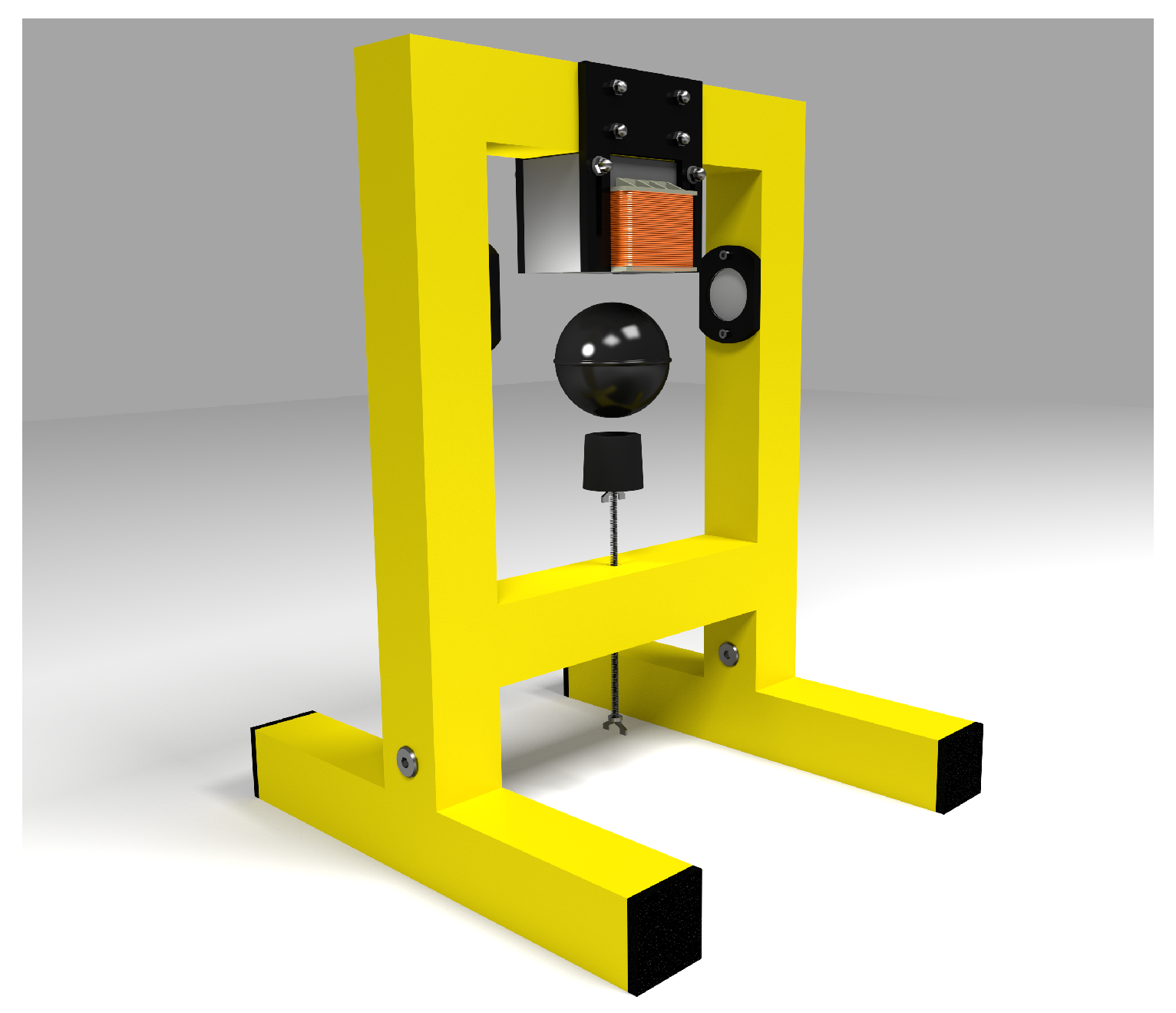
Figure 1.
Laboratory magnetic levitation system used in experiments. The system is offered by INTECO [22]. The light sensor measures the degree under which the light source is covered. The electromagnet is driven by a current driver.
Figure 1.
Laboratory magnetic levitation system used in experiments. The system is offered by INTECO [22]. The light sensor measures the degree under which the light source is covered. The electromagnet is driven by a current driver.

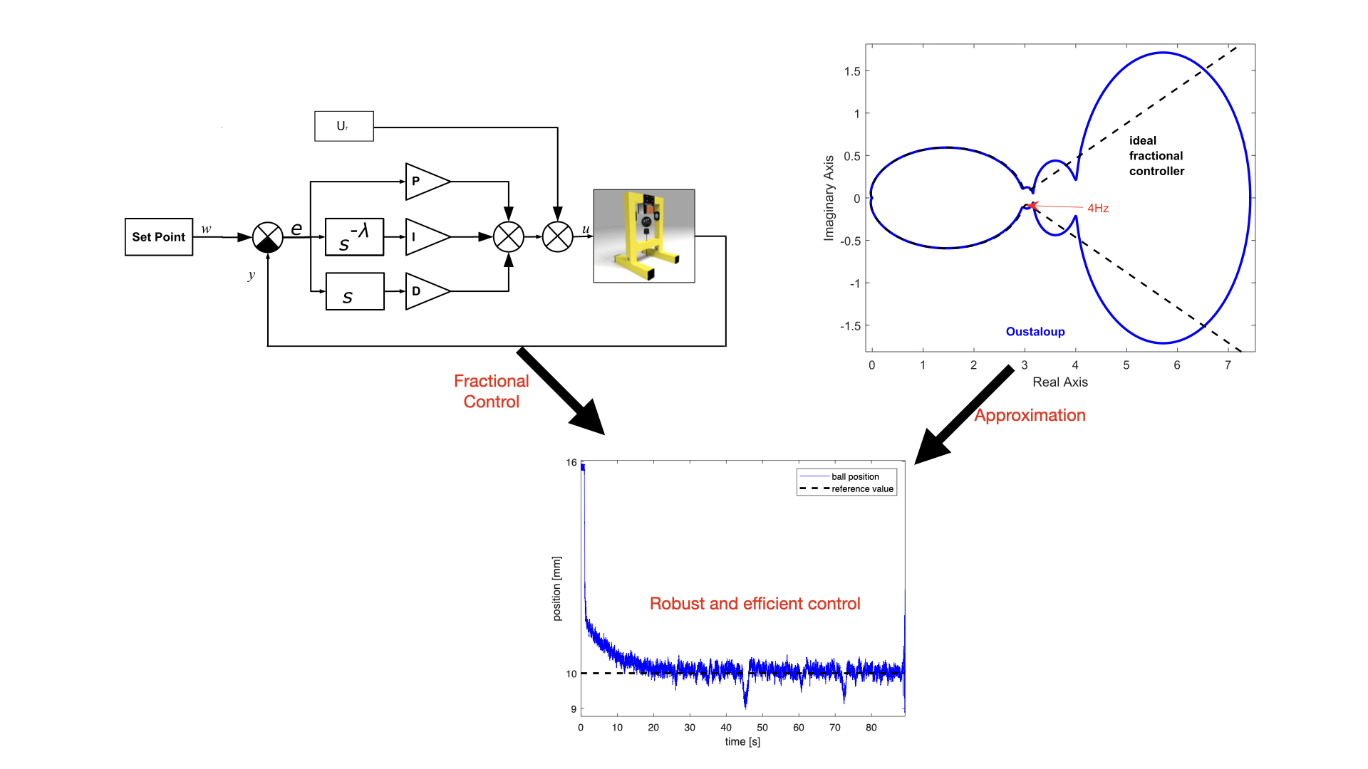
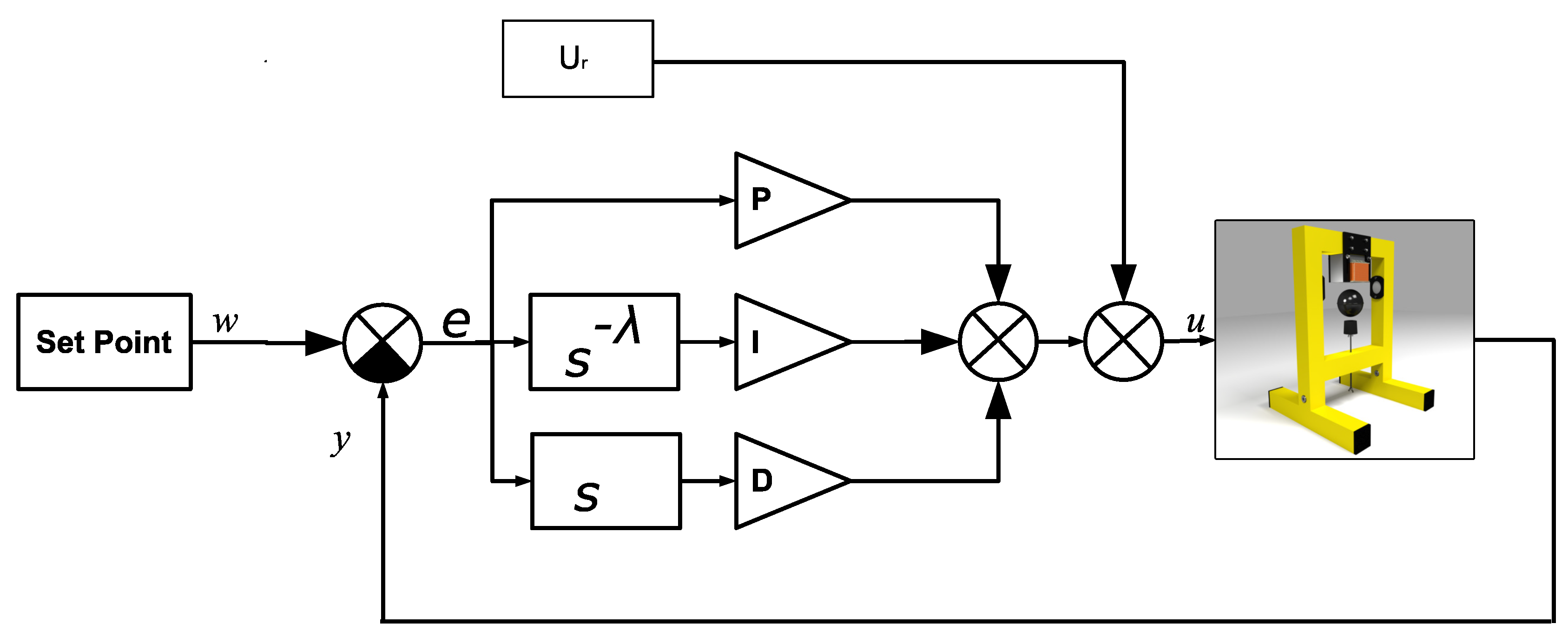
Figure 2.
Control loop schema for laboratory magnetic levitation with PID controller. In the diagram, we can see how to connect a regulator of a non-integer order and constant control value to laboratory magnetic levitation systems.
Figure 2.
Control loop schema for laboratory magnetic levitation with PID controller. In the diagram, we can see how to connect a regulator of a non-integer order and constant control value to laboratory magnetic levitation systems.

Figure 3.
Nyquist characteristics for a magnetic levitation system with the PID controller. The controller parameters are , , and . The analytical characteristics are marked by the black dashed line. The blue line represents the characteristic with the controller approximated by the Oustaloup’s method with parameters: order 5 and frequency bound between and . The cut-off frequency is marked in red on the chart for which the difference between the analytical system and its approximation can be observed.

Figure 4.
Result of the tuning system using simulated annealing for differing quality indicators. As can be seen in the case of Figure 4a,c, the controller allows the system to slightly overshoot. In these cases, the system also reaches the set point the fastest. In other cases, the system does not have any overshoots and moves slower to the operating point. However, the process is therefore smoother.


Figure 5.
Diagram of measuring the distance between the ball and the electromagnet, with marked distance orientation and a distance measuring system.
Figure 5.
Diagram of measuring the distance between the ball and the electromagnet, with marked distance orientation and a distance measuring system.

Figure 6.
(a) Ball position stabilization process with controller tuning by the analytic method, (b) ball position stabilization process with controller tuning by the SA method. (a) shows the process of stabilizing the position of the ball under the electromagnet with regulator tuning by the analytic method. The regulation time is approx. 1.5 s. The maximum overshoot is approx. 6 mm. When the working point is reached, vibrations are noticeable in its vicinity; (b) shows the process of stabilizing the position of the ball under the electromagnet with controller tuning by the SA method. The regulation time is approx. 2 s. There is no overshoot here. When the working point is reached, vibrations are noticeable in its vicinity.

Figure 7.
(a) Ball position stabilization process with disturbance for the controller tuning by the analytic method, (b) ball position stabilization process with disturbance for the controller tuning by the SA method. (a) shows the behavior of the control system with controller tuning by the analytic method for external disturbances. The ball in the vicinity of 2.5 s, 5 s, and 7s seconds is knocked out of the working point by a manual interaction. In each case, we see that the control system eliminates the disturbances. (b) shows the process of stabilizing the position of the ball under the electromagnet with controller tuning by SA method. The regulation time is approx. 2 s. There is no overshoot here. When the working point is reached, vibrations are noticeable in its vicinity.


Table 1.
Variables used in the mathematical description of a laboratory magnetic levitation system.
| Variable Name | Descritpion | Value |
|---|---|---|
| ball position | ||
| ball velocity | ||
| coil current | ||
| control voltage | ||
| m | ball mass | |
| g | gravitational acceleration | |
| gain of current driver | ||
| time constant of the linear current driver | ||
| zero error of current driver | ||
| positive constants identified for the plant. |
Table 2.
Result of tuning system using simulated annealing. The values of the parameter are similar in all cases. The ITSE indicator sets the highest gain for proportional and integral parts of the regulator. In contrast, the IAE indicator sets much lower gains on these parts, but similar gains on the derivatives. It does not change the fact that the quality indicators assume values from a similar range. The ISE and ISEDES indicators set a similar gain of proportional and derivative parts. On the other hand, ISEDES is a weaker integrator gain and therefore gives the worst final value of the quality indicator.
| Quality Indicator | Quality Value | ||||
|---|---|---|---|---|---|
| ISE: | |||||
| ITSE: | |||||
| ISEDES: | |||||
| IAE: |
Publisher’s Note: MDPI stays neutral with regard to jurisdictional claims in published maps and institutional affiliations. |
© 2020 by the authors. Licensee MDPI, Basel, Switzerland. This article is an open access article distributed under the terms and conditions of the Creative Commons Attribution (CC BY) license (http://creativecommons.org/licenses/by/4.0/).
Share and Cite
MDPI and ACS Style
Bauer, W.; Baranowski, J. Fractional PIλD Controller Design for a Magnetic Levitation System. Electronics 2020, 9, 2135. https://0-doi-org.brum.beds.ac.uk/10.3390/electronics9122135
AMA Style
Bauer W, Baranowski J. Fractional PIλD Controller Design for a Magnetic Levitation System. Electronics. 2020; 9(12):2135. https://0-doi-org.brum.beds.ac.uk/10.3390/electronics9122135
Chicago/Turabian StyleBauer, Waldemar, and Jerzy Baranowski. 2020. "Fractional PIλD Controller Design for a Magnetic Levitation System" Electronics 9, no. 12: 2135. https://0-doi-org.brum.beds.ac.uk/10.3390/electronics9122135
Note that from the first issue of 2016, this journal uses article numbers instead of page numbers. See further details here.