
Profitability of Residential Battery Energy Storage Combined with Solar Photovoltaics

1
Chair of Business Information Systems, Technical University of Munich, Boltzmannstr. 3, 85748 Garching, Germany
2
Munich School of Engineering, Technical University of Munich, Lichtenbergstr. 4a, 85748 Garching, Germany
*
Author to whom correspondence should be addressed.
Energies 2017, 10(7), 976; https://0-doi-org.brum.beds.ac.uk/10.3390/en10070976
Submission received: 9 May 2017
/
Revised: 6 July 2017
/
Accepted: 6 July 2017
/
Published: 11 July 2017
(This article belongs to the Special Issue Energy Efficient and Smart Cities)
Abstract
:Lithium-ion (Li-Ion) batteries are increasingly being considered as bulk energy storage in grid applications. One such application is residential energy storage combined with solar photovoltaic (PV) panels to enable higher self-consumption rates, which has become financially more attractive recently due to decreasing feed-in subsidies. Although residential energy storage solutions are commercially mature, it remains unclear which system configurations and circumstances, including aggregator-based applications such as the provision of ancillary services, lead to profitable consumer investments. Therefore, we conduct an extensive simulation study that is able to jointly capture these aspects. Our results show that, at current battery module prices, even optimal system configurations still do not lead to profitable investments into Li-Ion batteries if they are merely used as a buffer for solar energy. The first settings in which they will become profitable, as prices are further declining, will be larger households at locations with higher average levels of solar irradiance. If the batteries can be remote-controlled by an aggregator to provide overnight negative reserve, their profitability increases significantly.
1. Introduction
The generation of electricity using residential-size solar photovoltaics (PV) installations has reached grid parity in 19 markets globally, including countries with relatively low levels of solar irradiance such as Germany [1]. Today’s levelized cost of solar energy without subsidies is therefore smaller than the cost of purchasing energy from the utility. Until recently, PV systems were mainly installed to feed the generated electricity directly into the grid at a fixed feed-in remuneration that is guaranteed for usually 20 years. Today, the solar PV feed-in remuneration ranges below the end-consumer prices in many countries worldwide, which is making self-consumption of solar power more attractive.
Although solar energy and most of the demand in households occurs in the daytime, the simultaneity of solar power and demand is limited. Besides controlling deferrable loads, e.g., hot water heaters and washing machines, battery energy storage is increasingly being considered as an effective way to increase self-consumption. Several companies, including electric vehicle manufacturer Tesla (San Carlos, CA, USA) [2], offer lithium-ion (Li-Ion) batteries as a buffer for solar energy so that excess PV generation can be stored in the battery for self-consumption during times when demand exceeds supply. Li-Ion battery cell prices are declining rapidly, while their lifetime is slowly increasing [3]. Therefore, investing in Li-Ion battery storage will become financially more attractive in the future. However, it still remains an open research question how systems should be sized and operated to achieve positive business cases. Moreover, considering the high cost of Li-Ion battery cells, being able to utilize residential batteries for more than just buffering solar energy could be a major driver of profitability. Their ability to quickly adjust (dis)charging power makes batteries a potential provider of ancillary services. Controlled by an aggregator or directly by the system operator, distributed batteries could, for instance, help to provide frequency reserve.
In this paper, we investigate the financial impact of coupling state-of-the-art Li-Ion batteries with solar PV panels in residential settings. We make the following contributions:
- We advance beyond conventional methodology by simulating stochastically the electricity demand of different households and PV generation at different locations in high temporal resolution.
- In addition to solar energy buffering, we investigate the use of batteries to provide negative reserve and its impact on profitability, which is a largely unexplored topic.
- We implement a detailed model to control the operation of a residential energy system and derive the net present value (NPV) of different system configurations.
- Based on the results of an unprecedented large number of experiments with different inputs, we conduct a sensitivity study to identify optimal system configurations and the drivers of energy storage profitability.
- Our study provides fresh insights that facilitate investment decisions, in particular which system configuration should be chosen based on location, household size, and current battery module price.
This paper is organized as follows: in Section 2, we review related literature. Section 3 provides details on the different models and data we use. In Section 4, we summarize the setup and results of a comprehensive simulation study. Section 5 discusses our work, including its limitations and possible future work. Finally, in Section 6, we provide summarized conclusions of our study.
2. Related Work
Several recent studies [4,5,6] attempted to examine the profitability and optimal sizing of residential PV-battery systems, but most suffer from major limitations that impede the robustness of the results. A common shortcoming stems from the use of low time resolution electricity demand and PV generation models, which fail to capture the short-time peaks that are intrinsic to real generation and load curves. The time-averaging effects arise from coarse resolution models, lead to inaccurate representation of the instantaneous matching of electricity supply and demand, and, consequently, undermine the capacity sizing and economic assessment of PV-battery systems. Based on the simulation of a UK household over a summer day, the authors of [7] reported significant errors in the estimation of on-site solar fraction by coarse time resolution models. An hourly resolution model overestimated the PV supply and demand matching capability by over 60% compared to a minute-resolution model. Ried et al. [8] modeled the profitability of PV-battery systems for a sample of households and reported significant underestimation of battery cycle life using coarse time resolution models. An hourly resolution model on average underestimated the battery cycle by 9% and overestimated the battery life by up to three years compared to a minute-resolution model. Furthermore, past studies neglected the stochasticity in residential electricity demand and drew conclusions merely based on simulations using standard load profiles of a single household. Ried et al. [8] reported considerable errors in the estimation of battery cycle life and overall cost-savings when standard load profiles as opposed to measured household demand curves are used. In the following, we provide several detailed reviews of key papers related to our work.
Naumann et al. [4] investigate the costs of Li-Ion battery storage for a 4-person single family house under the current regulatory regime in Germany. They scale and linearly interpolate a low granularity standard load profile (15 min averages, 4-person household) to obtain one-minute household demand. Instead of searching the optimal combination of PV and battery sizes, they fix the PV capacity (4.4 kWp) and conduct a sensitivity study of the return on investment (ROI) of the system in three battery size scenarios. With the PV size constraint, they reported an optimal battery capacity of 4.4 kWh while the ROI varies depending on assumptions in the state of health and aging behavior of the batteries.
Weniger et al. [5] attempt to find optimal PV and Li-Ion battery sizes for a 3-person single family house in Germany. They use measured data of typical daily load profiles from one household in one minute resolution based on VDI (verein deutscher ingenieure) guideline 4655 [9], which they assemble into a one year long profile. The main caveat of the study arises from the very conservative assumptions regarding the battery modules, in particular costs ranging between 3000 EUR/kWh and 600 EUR/kWh, state of charge ranging between 20% and 80%, and a cycle life of 5000 equivalent full cycles. As a result, PV-battery systems are found to be economically viable only in the long term assuming PV system costs of 1000 EUR/kWp, battery costs of 600 EUR/kWh, and feed-in tariffs as low as 0.02 EUR/kWh. The authors reported an optimal configuration consists of (per MWh of demand) a 0.8 kWp PV system and 1.1 kWh usable battery capacity.
The authors of [6] conduct a very detailed study of the profitability of residential lead-acid batteries. In particular, they use several learning curve models to forecast system costs (one for each major system component) and different price development scenarios to investigate how net present values would evolve if investments were made anytime between 2013 and 2022. In contrast to the authors of [4], they consider optimal PV panel and battery sizing. However, they use hourly solar data and concatenated standard load profiles (15 min resolution) as input for their simulations.
Zhu at al. [10] investigate the use of residential batteries for exploiting time of use (TOU) tariffs. TOU tariffs are end-customer contracts that result in different electricity prices based on when electricity is consumed. In contrast to us, they consider two different battery types with different cost characteristics being operated simultaneously, a lead-acid and a lithium-ion battery. This can lead to higher cost-efficiency due to optimal coordination. Moreover, they do not consider optimal battery sizing and combined use with solar PV, which is the focus of this paper.
The authors of [11] developed a method for optimally sizing PV-battery systems based on a probabilistic (“chance constraint”) approach. Similar to [12], which their formal analysis is based on, they consider autonomous energy systems without grid connection. In contrast to the grid-connected systems investigated in our paper, such scenarios call for an investigation of how a probabilistic metric of autonomy, i.e., how likely a certain system configuration would be able to cover all demand, can be provided. In [11], such a method is proposed. However, to be used in practice, one needs to carry out stochastic simulations based on actual data, such that the complex time-dependent system behavior can be considered.
In this paper, we try to combine the strengths and overcome the weaknesses of the past studies. In particular, we use recent data-driven models to simulate stochastically the electricity demand of households and PV generation in high time resolution in an effort to accurately assess the profitability of residential PV-battery systems. We also consider a large sample of households in different sizes and PV generation in different locations to ensure generalizable results. In fact, our results show that these contextual parameters are decisive to the profitability of PV-battery systems. Similar to [5], our work considers the important financial trade-offs resulting from different PV panel and battery sizes by searching for optimal configurations instead of fixing them ex ante. However, we use more realistic input assumptions and stochastic residential load profiles that are lacking in [4,5]. Furthermore, our paper also investigates a realistic extension of the standard residential battery use case, namely the provision of negative reserve. This application is recognized to have growing market potential worldwide but has not been considered in previous publications [13].
3. Models and Data
3.1. Household Load Model
We use the residential electricity demand model described in detail in [14] to generate random load profiles. The model uses an activity-based modeling technique which combines data from a time use survey with smart meter data of household appliances to derive realistic load profiles on the household level at one-minute resolution. Load is computed using a bottom-up approach. Empirical data about timing and duration of activities (e.g., cooking, watching TV, etc.) is combined with empirical data on load distributions depending on household size to derive so-called activity load profiles of households. These profiles are stochastic, since the use of each activity-based load is simulated by sampling from the corresponding probability distributions. One of the special merits of this model is that it also considers the shape of standard load profiles. It achieves this by making sure that the mean of many simulated household load profiles converges to the standard load profile. The authors of [14] have validated the generated household load traces by comparing them to actual smart meter measurements based on critical statistical properties.
3.2. Solar PV Model
We apply models described in [15,16] to obtain realistic data traces for the DC power generated by residential solar crystalline silicon PV panels. PV module efficiency can be approximated using Equation (1) [15], where and G are input variables denoting the PV cell temperature and incident solar irradiance on the PV array, respectively. The remaining parameters are constants as provided in Table 1:
The PV module temperature can be modeled according to Equation (2) [16], where and are variables representing ambient temperature and wind speed, respectively:
The total DC power output of a PV module can be calculated as , where is the module area.
We use Meteonorm [17] to create data traces for a typical year (1991–2010) in one-minute resolution. Meteonorm provides simulated ground measurements of solar irradiance for typical years, i.e., it considers the short-term effect of moving clouds. Meteonorm was configured to simulate G over a year, assuming a south facing PV panel tilted by 30°, which represents the optimal fixed tilt position in Central Europe. We also use Meteonorm to obtain data traces of the ambient temperature and wind speed . Data was generated for two locations in Germany, Bremen and Munich. We have chosen these locations since Bremen has one of the lowest, whereas Munich one of the highest solar irradiance levels in Germany. The results obtained for these two extreme locations enable us to estimate the impact of solar availability on the profitability of PV-battery systems. We scale the resulting DC power generation traces based on the maximum value observed during one year and the desired peak power capacity, .
3.3. Battery Model
Our battery model can be defined using the following parameters: The battery efficiency (charging and discharging), the nominal battery storage capacity , and the C-rates for charging and discharging, and . In addition, we define the usable range of the state of charge (SOC) of the battery via and .
The overall lifetime of Li-Ion batteries can be approximated based on two parameters, the calendar lifetime and the maximum number of full battery cycles until decommissioning . Lifetime parameters differ depending on the battery chemistry. In this work, we consider the lithium iron phosphate (LiFePO4) battery chemistry, which is used by several solar battery providers [18,19] due to their long cycle life and operational robustness (depth of discharge, safety, temperature, etc.). The exact specifications were based on the Sony Fortelion cell (Tokyo, Japan) [20]. The capacity of LiFePO4 batteries decreases approximately linearly with time until a certain reflection point, beyond which capacity rapidly declines. We denote the end of life battery capacity by . The SOC range of these cells are not restricted in practice, because, in contrast to other battery chemistries, depth of discharge does not play a major role in the aging process of LiFePO4 cells [21].
3.4. Power Electronics Model
To transform the DC power from the solar PV panel and the battery into AC power used by household appliances and the grid, an inverter is required. Likewise, charging the battery with grid power requires rectification of AC grid power to DC battery charging power. Power electronics efficiency usually peaks at its rated output power and decreases in other load conditions. To accurately consider this behavior, we use the following model provided in [4]:
The rated output power is treated as a constant. In the following, we will model two power electronic devices: the inverter that converts DC power from the panel and the battery into AC power and the rectifier required to convert AC grid power to DC charging power for the battery. The nominal power electronics capacity is chosen to be equal to expected peak load. Therefore, in the former and in the latter case.
3.5. Battery Control
We combine the different models described above to perform a comprehensive evaluation of state-of-the-art residential battery energy storage. In addition to using the battery as a way to store excess solar PV energy and use the stored energy to (partially) replace power drawn from the grid, we also investigate the case of charging the battery using grid power during times of negative reserve deployment.
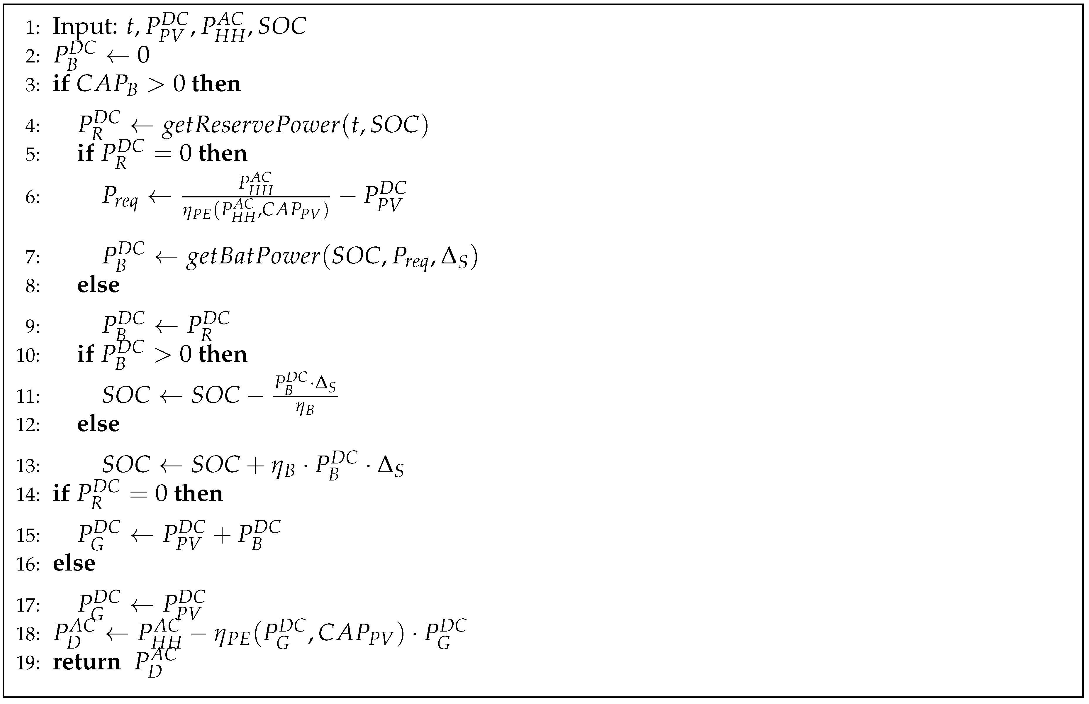
Figure 1 shows the algorithm of method , which takes the following inputs: the current time t, solar PV generation , household demand , and the battery’s SOC. It controls the battery power during the control time interval by determining a feasible value for the DC battery power . Thus, the control frequency depends on the length of , which is set to 1 min in our evaluations. We assume that all control inputs are measured or are accurately estimated based on available measurements. Inputs have to be provided to the algorithm at the same frequency as controls are computed. Apart from computing , the battery control algorithm also returns the remaining power that needs to be transferred to or from the grid. If is positive, additional power needs to be drawn from the grid to cover the demand. If negative, excess energy produced by the solar PV panels that cannot be absorbed by the battery is fed back into the grid.
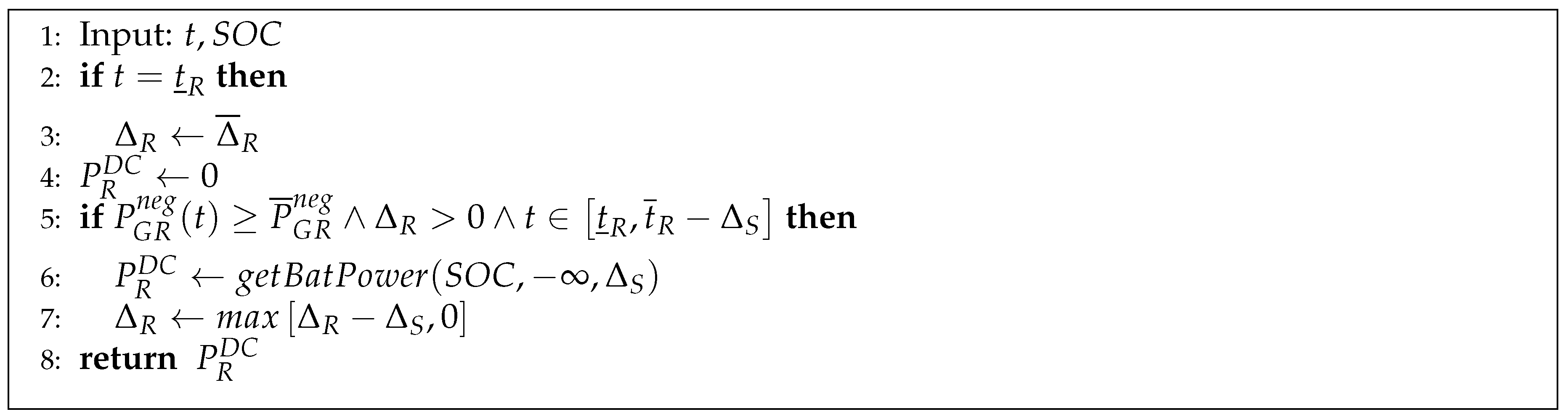
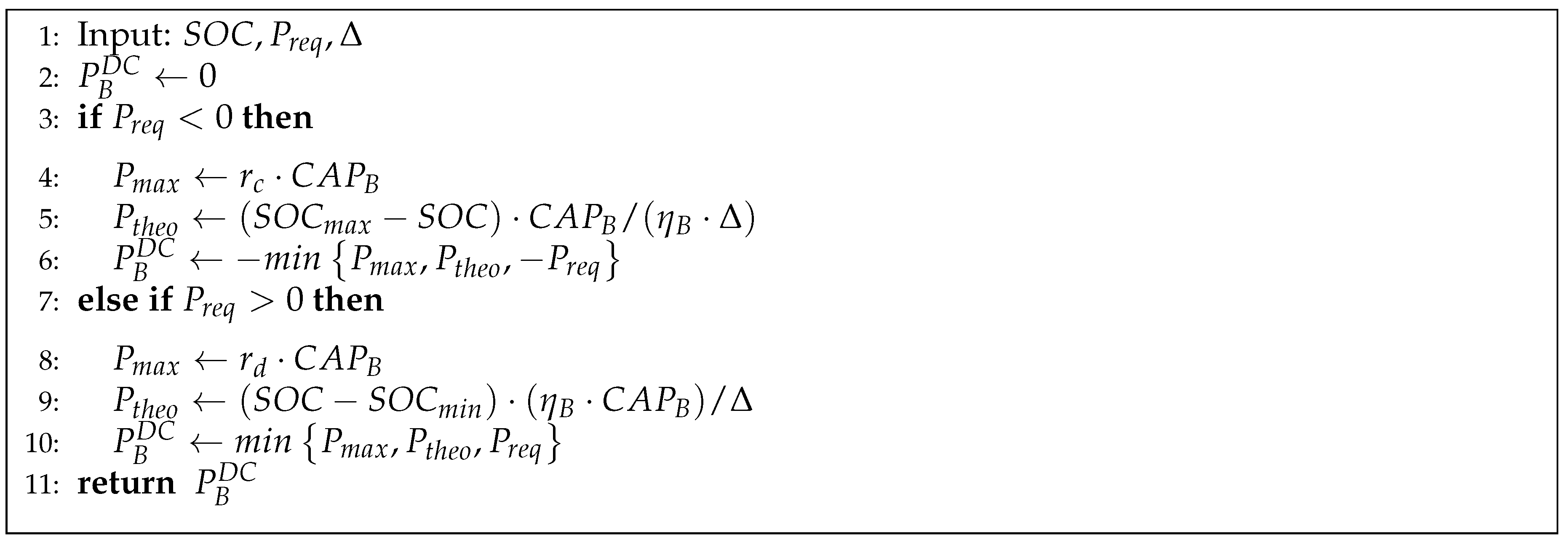
Lines 3–9 of algorithm determine the battery dispatch, i.e., the value of . The method provided in Figure 2 determines a feasible reserve contribution of the battery, which requires the battery state, and can otherwise be based on time, reserve requirements, etc. In Germany, there exist separate markets for positive and negative secondary reserve, from 8 a.m. to 8 p.m., and from 8 p.m. to 8 a.m. the next day. The underlying market mechanism is a pay-as-bid auction for capacity and actual energy delivery. The corresponding Internet-based market platform [22] is run jointly by the German Transmission System Operators (TSOs). Any business party able to fulfill the technical qualification criteria (including minimum power and response time) can participate in these markets. More details about the German ancillary services markets can be found in [23]. In this paper, we evaluate negative reserve provision in min time intervals between p.m. and a.m., which corresponds to the current rules for participating in the secondary reserve market in Germany. Furthermore, we assume that, during each of these 12 h intervals, batteries can charge for at most h, which can result in one full recharge at a charging C-rate of one. If the battery is scheduled to deliver reserve energy, i.e., the determined reserve power level is not equal to zero, the battery is exclusively used for this purpose. Otherwise, it is used to absorb excess solar energy or provide energy if the household demand is higher than PV generation.Figure 3 specifies the algorithm we use to determine feasible battery power based on the SOC, the required power , and the time interval used for charging or discharging.
Figure 4 shows selected input traces and simulation results to demonstrate the effect of the applied battery control strategies. Ten single-person household traces are plotted at once to reveal the stochasticity of the demand and how it leads to different battery utilization patterns. One can also see that negative reserve is required very often, i.e., the chances that batteries can be controlled to provide it during the allowed time interval are very high.
4. Simulation Study
To perform a comprehensive profitability evaluation of the residential battery energy storage, we run a large number of simulations with different parameter configurations. Each simulation run covers one entire year in one minute detail, i.e., the computational steps summarized in algorithm control (cf. Figure 1) have to be executed times in each run. Since we intend to consider a typical investment horizon of 20 years, we scale the PV module and battery capacity to average values, i.e., and , where % is the annual (linear) performance loss of solar PV cells according to [24]. Thus, for the NPV calculations the full detail of minute calculations is considered because the energy values , , , and are calculated using the method described above. However, we simulate one year per configuration, and then use the resulting energy values to estimate net present value (NPV) for longer time periods.
To compute the figures of merit presented in the following, we collect several aggregated metrics in each simulation run, including the total energy consumed by the household , the energy from the grid and the excess solar energy being fed into the grid, . In addition, we compute the total energy being provided by the battery.
4.1. Metrics
We evaluate the profitability of different combinations of solar PV panel and battery sizes by computing the NPVs of the corresponding investments. NPV is one amongst several ways to determine the return of an investment (ROI). In contrast to the most basic ROI formula, i.e., the difference between the gain from an investment and the cost of investment, and the cost of investment, the use of NPV allows us to consider the time value of cash flows in subsequent time periods, which is particularly important for long investment horizons. In our case, significant investments are due right at the beginning of the considered investment time period, whereas revenues are constantly being generated during a relatively long time (20 years). Thus, even relatively low interest rates may play a crucial role in the decision. Furthermore, the NPV method provides a monetary value instead of merely measuring the efficiency of an investment in terms of a percentage rate and is thus more informative.
The corresponding financial parameters are summarized in Table 2. All price values exclude the value added tax (VAT).
Based on these values, we calculate initial investments into the different system components based on their respective sizes, in particular and . The nominal capacity of the PV inverter and grid-to-battery rectifier used during reserve provision are derived from these values. Thus, the initial investment costs for the solar modules (Equation (4)), the battery (Equation (5)), and the additional power electronic equipment (Equation (6)) can be calculated as follows:
Since both the power electronic equipment and the battery modules usually have a shorter lifetime than the assumed investment horizon of 20 years, we consider their replacement costs in the NPV calculation. Furthermore, since we examine a limited investment horizon, we also consider the residual value of assets at the end of the investment period. Otherwise, the replacement of a system component shortly before the investment horizon ends would distort the NPV. Replacement costs and residual values include VAT, but exclude additional (de)installation costs. We denote the annual cash flow resulting from solar PV system replacement costs and residual value in year t by . The cash flow resulting from the investment in the battery modules is denoted by , the cash flow corresponding with the investment in additional power electronics required for reserve provision by . Replacement times are determined from the parameters , , and . Residual values are determined proportionally, i.e., the residual value of device D that costs EUR, has lifetime , and was installed or last replaced at time , would be equal to . In addition to the equally distributed replacement costs, we consider annual PV system maintenance costs according to Equation (7):
Positive cash flows correspond to revenues resulting from the grid electricity cost savings and the revenue from PV feed-in. In Germany, households are paid a fixed feed-in tariff for the PV energy they deliver to the grid. The tariff is determined at installation time and remains valid for 20 years. More details can be found in the corresponding Act on the Development of Renewable Energy Sources [26]. Since households have to pay VAT on self-consumed electricity, the complete annual revenue can be obtained using Equation (8):
The net present value of an investment into a residential energy system that is composed of PV module, battery, and power electronic equipment is given in Equation (9). If this value is positive, the investment would be beneficial compared to the non-investment alternative, and disadvantageous otherwise:
In addition to net present values, we compute the number of annual storage cycles according to Equation (10) and the self-sufficiency rate according to Equation (11):
In the case of reserve provision, i.e., , the total energy drawn from the distribution grid includes the reserve energy. Thus, we still define self-sufficiency as the percentage of used energy that is produced on-site, even if charging during reserve provision is assumed to be free. We do not assume that the aggregator pays the home owner extra for being able to control battery charging, i.e., the NPVs computed for represent lower bounds. Market participation operations of the aggregator, in particular the control of many batteries in concert with other energy resources forming a virtual power plant, are beyond the scope of this paper [27]. Provided that the aggregator fulfills the requirements for participating in the reserve market, it should be able to obtain (positive) revenues from the participation. However, based on historical price data, these revenues should be rather limited today [28]. The deployment bids would have to be sufficiently low, such that the aggregator would be instructed to deliver reserve energy relatively often, which, in turn, is required to recharge the batteries overnight.
4.2. Setup
Table 3 lists the sensitivity parameters considered in this study. All parameters except the battery module price require independent simulations. To account for the stochasticity of household load and its impact on self-consumption and battery operation, we perform ten independent simulations for each parameter configuration and report the mean metrics.
4.3. Implementation
Our simulation and data processing procedures can be divided into three phases.
In the first phase, we use appropriate models to generate the input data traces. We use the original implementation of the household load model described in Section 3.1 to generate a large number of year-long household consumption traces in one-minute resolution for different household sizes. Using the weather data traces generated by Meteonorm, we compute corresponding PV power generation using our own Python implementation of the models described in Section 3.2. The reserve traces were obtained from [29].
In the second phase, we simulate the PV-battery systems over the course of a year in one minute detail. Even at 1 kWp increments of PV capacity and 1 kWh increments of battery capacity, we still need to perform 1056 simulation runs. Due to the high time granularity, the inclusion of many independent household demand traces per run (cf. Figure 4), and the required computation in each simulation step (cf. Section 3.5), each simulation run takes several hours on commodity hardware. Using two powerful computer servers with 32 cores each, we were able to parallelize simulations such that the full experimental setup was feasible in reasonable time.
In the final phase, we calculate the figures of merit, in particular, net present value, annual storage cycles, and self-sufficiency rates using Python scripts. This enables us to perform sensitivity studies using different financial parameters (cf. Table 2) without having to repeat the computationally expensive simulations of the second phase.
4.4. Results
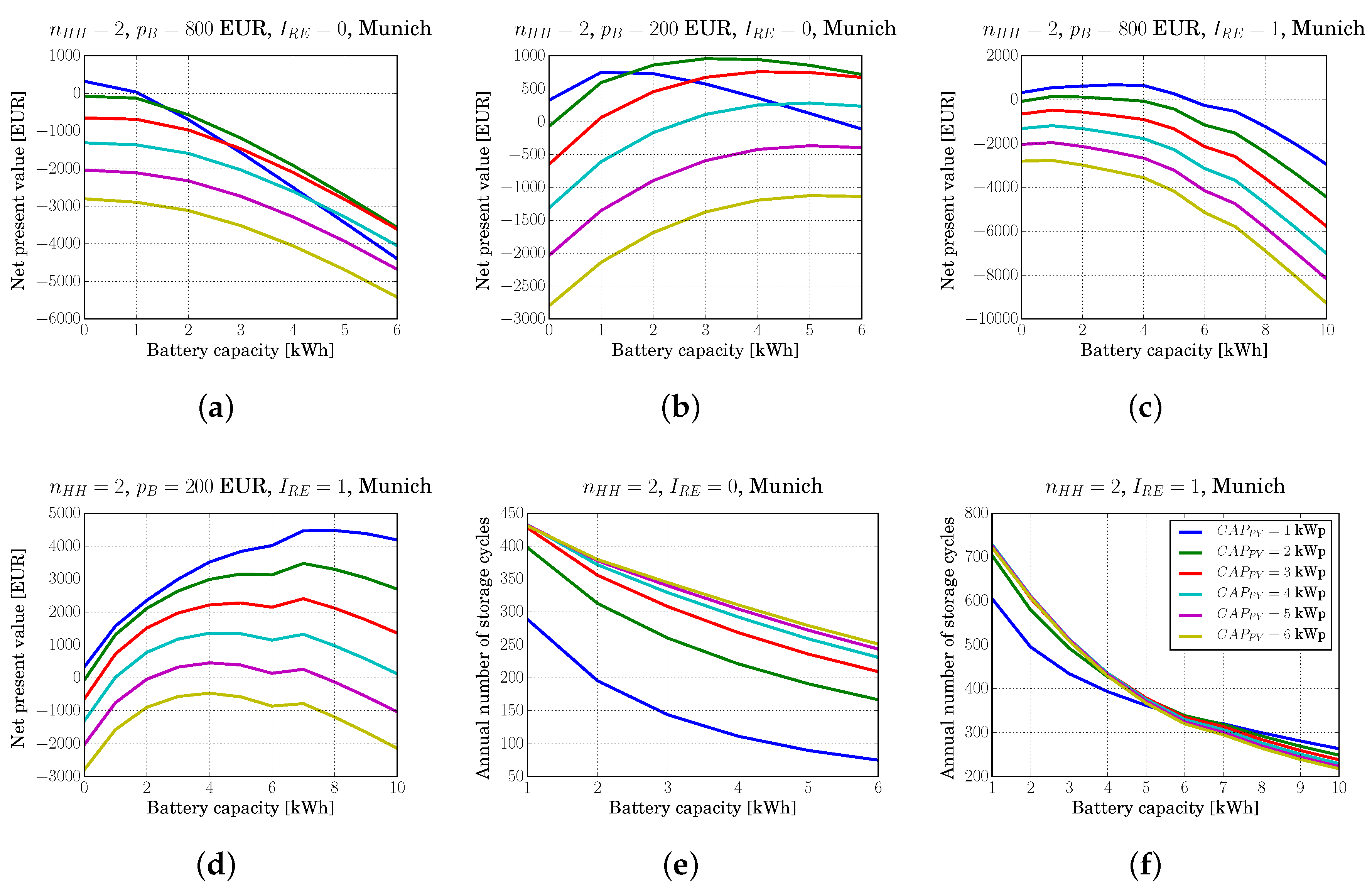
Figure 5 contains plots of net present values and number of annual storage cycles for two-person households in Munich. These plots only represent a fraction of the total results we obtained. The figures reveal several important facts about the optimal sizing of system components and the influence of battery prices and reserve provision, which are outlined in the following. At current battery prices of 800 EUR/kWh and without reserve provision, it would be optimal to invest only into a system consisting of a small PV module without a battery. Investing into energy storage would only reduce profitability in this case. Even at very low battery prices of 200 EUR/kWh, NPV peaks at rather small storage capacities in the range of 1 kWh–4 kWh. The possibility of a free overnight recharge resulting from negative reserve provision significantly increases profitability, despite approximately doubling the number of annual storage cycles. In this case, the optimal energy storage capacity also increases, but still peaks well below 10 kWh.
Across all cases, it becomes clear that relatively small PV module capacities (1 kWp–2 kWp) are more beneficial from a financial perspective. Although additional energy storage capacity can, as expected, significantly increase the value of PV capacity, system configurations with more than 2 kWp of PV capacity will remain less profitable than smaller systems, irrespective of energy storage. Similar trends are observed in other household scenarios and for Bremen.
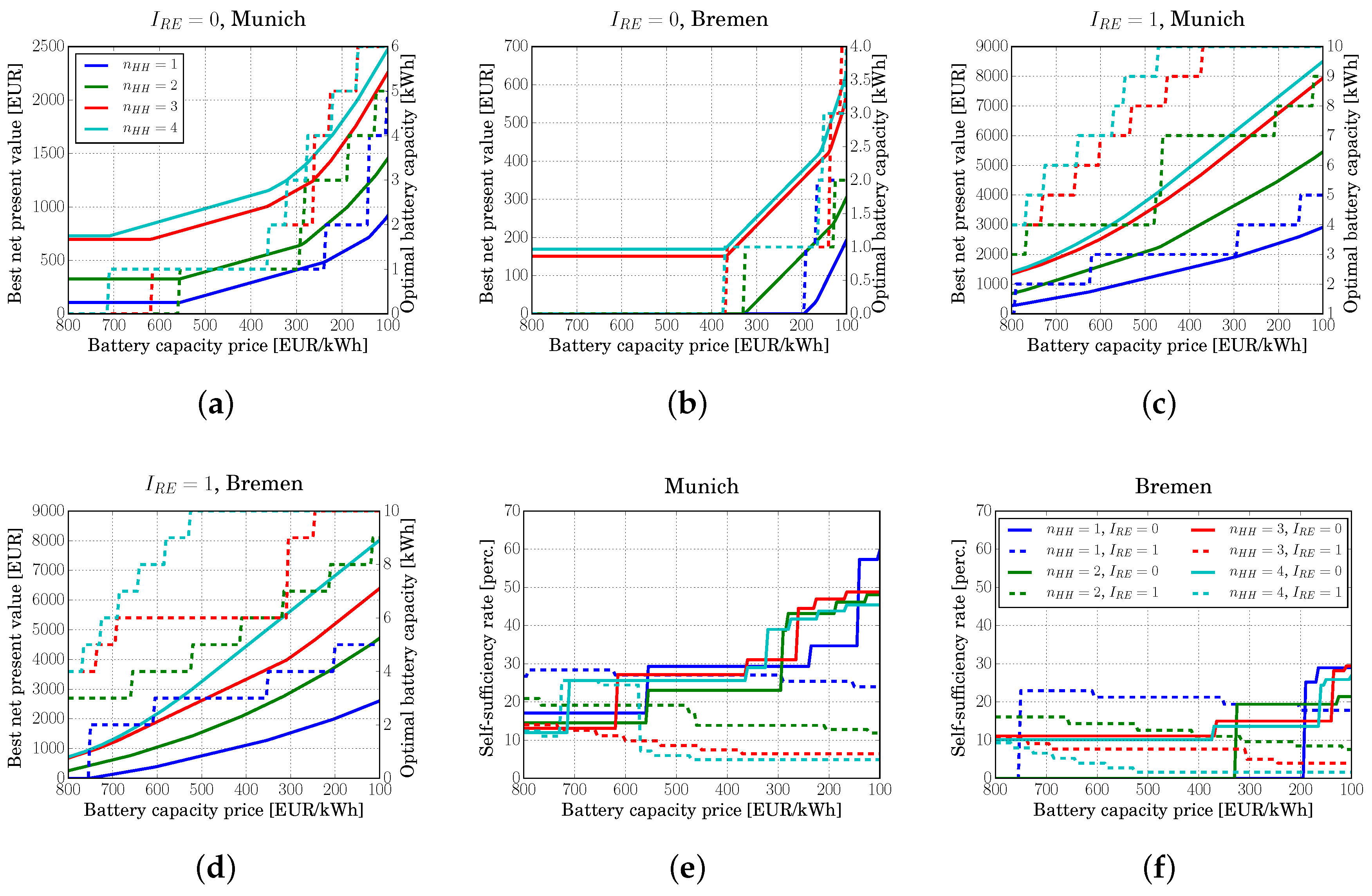
In Figure 6, colors refer to different household sizes (1 person–4 persons), whereas solid and dashed lines designate different metrics, including NPV, battery capacity and self-sufficiency rate. Figure 6a–d show the best NPVs (solid lines) within the search space defined in Table 3, as battery prices decrease from 800 EUR/kWh to 100 EUR/kWh. The figures reveal at which price levels investments in energy storage become profitable in the studied cases. Taking Figure 6a as an example, for a 3-person household, it is more profitable to have a solar PV system without a battery when the battery price is above 600 EUR/kWh. This can be observed as the optimal battery capacity (red dash line) stays at zero when the value of the x-axis is beyond 600. When the battery price drops to between 300 EUR/kWh and 600 EUR/kWh, a small battery of 1 kWh capacity is optimal (red dash line reaches 1). The optimal battery capacity increases in steps up to 6 kWh as the battery price drops to 100 EUR/kWh. The contextual factors also play a crucial role as NPVs increase substantially with larger household size and higher solar availability.
Interestingly, irrespective of how low the prices per kWh of energy storage capacity become, capacities greater than 6 kWh are never an optimal choice in the regular self-consumption use case. If the batteries deliver negative reserve, however, optimal battery sizes approximately double. Furthermore, although battery owners are not financially compensated directly, reserve provision significantly increases profitability.
Figure 6e,f show self-sufficiency rates for the cases without and with reserve provision (solid and dashed lines, respectively). Whereas the use of additional energy storage capacity at decreasing battery prices leads to higher self-sufficiency, the opposite is true if batteries deliver negative reserve. The reason is that the amount of energy being charged into the battery in response to reserve provision starts dwarfing the amount of solar energy being buffered. A self-sufficiency rate of 0% indicates that it is financially optimal not to invest in either solar PV modules or battery storage.
5. Discussion
Using a high resolution stochastic electricity demand model, we are able to quantify the effects of household size and solar availability on the profitability of PV-battery systems. Although these contextual factors have proven to be important in our findings, they were largely neglected in previous studies.
Furthermore, we explore the impact of providing negative reserve using the batteries (cf. Section 1), which is a timely topic in Europe. The way the aggregator controls the batteries to provide reserve in our use case is simple but realistic. The optimization problem of scheduling large numbers of energy storage devices in accordance with German market rules has been studied in another publication [27], and would exceed the scope of this work. In this paper, we thus make the simplifying assumption that batteries can be charged at nominal charging power as long as there is actual demand for negative reserve (usually many MWs). We used a real one year long trace of negative reserve to make sure that our results could actually materialize in practice. Given the case we consider, i.e., reserve provision during a 12 h long time interval with a maximum charging time of 1 h, batteries would almost certainly be able to recharge every night. The required switching and metering infrastructure on the customer side would be basic and inexpensive.
Since the power output of lithium-ion batteries can change almost instantaneously based on the attached load or power supply, considering the ramp rate of the modeled energy storage is not required here. However, it could be an issue if other types of energy storage are modeled or if the time granularity of our analysis were much higher. Moreover, considering different reserve provision use cases, including ones involving the discharge of batteries, could be valuable future work.
The data and assumptions adopted in this study have been carefully selected to cover a representative range of values in reality in order to ensure generalizable results. Furthermore, by leveraging an advanced method for generating representative household load traces [14], we are able to take stochastic effects into account. Whereas these features distinguish our study from previous work, they also lead to high computational complexity, which we manage by deploying our code on large servers and taking advantage of full parallelization. The results clearly show that the stochasticity of household consumption patterns are important to consider as they have significant impacts on the NPVs, and in turn, the optimal system configurations. In this paper, we have not explicitly shown the impact of data granularity on the matching of solar PV energy production and household demand because we feel that this is beyond the scope of this paper. The general importance of data granularity in the context of our study has already been shown in the literature [7].
We do not consider learning curves in this work, which form an integral part of related works [6]. Learning curves represent the impact of learning over time, e.g., on costs or prices. In the context of our study, the prices of residential energy generation and storage systems may decrease over time, e.g., due to economies of scale and increasing competition. Instead, we implicitly assume that PV panel and power electronics prices will not dramatically decrease in the future. Energy storage price, however, is treated as a sensitivity parameter in our study without making explicit predictions about when which price level will be reached, since we believe that such predictions are highly speculative at this time.
Our sensitivity study can also be used to assess the impact of subsidies for residential energy storage. A recently prolonged subsidy program supporting residential battery energy storage in Germany promises a payment depending on the size of the solar PV module and battery module initial investment cost , which can be calculated according to EUR [30]. Thus, assuming the current battery cost of 800 EUR/kWh, the subsidy for a 1 kWp PV module with a 1 kWh battery would be approximately 200 EUR. Considering the results shown in Figure 6a,b, this subsidy would be sufficient to make battery investments for larger households (three and four persons) at locations with high irradiance levels, like Munich, profitable. However, our results show that it is insufficient to foster storage adoption in other cases.
Time-of-use (TOU) tariffs, i.e., contracts that result in different electricity prices based on when electricity is used, are common in some countries, in particular in the US [31]. Typically, TOU tariffs lead to higher charges at times of peak demand, i.e., at mid-day, and lower charges otherwise. They require “smart" meters capable of time-based demand measurement and vary in terms of specified pricing periods and levels. In Germany, smart meters have not yet been rolled out at the household level, thus German utilities do not offer TOU tariffs so far. Since residential energy storage reduces electricity usage during times of potential peak demand (cf. Figure 4), we expect TOU pricing to have a positive effect on its profitability. However, since TOU can be very different based on the demand shifting goal of the utility and a significant study is therefore beyond the scope of this paper, we recommend a self-contained follow-up study that specifically investigates this issue.
We can confirm that financially optimal system configurations for self-consumption scenarios imply relatively small solar PV and battery capacities. Even if battery prices halved from today’s 800 EUR/kWh price level to 400 EUR/kWh, optimal battery sizes would still range at approximately 1 kWh (cf. Figure 6a), although much larger residential batteries are offered already today (e.g., Tesla’s Powerwall has a storage capacity of 6.4 kWh [2]). This result generally corresponds with the findings of previous studies, in particular [5]. Furthermore, we find that battery module prices would have to further decrease from today’s levels to make first investments in residential energy storage profitable. For instance, at locations near Munich, initial investments into energy storage would become profitable at prices lower than 550 EUR/kWh for all household sizes (cf. Figure 6a), whereas prices would have to decrease below 200 EUR/kWh to lead to profitable investments near Bremen (cf. Figure 6b). However, as our detailed results have shown, the exact “break even” battery prices and the optimal system configurations vary substantially depending on factors such as household size and solar availability. We thus believe that it would be dubious to quote such numbers without considering these contextual features.
The weather and time use data used as input to the household load model assume siting in Central Europe, which determines the results of the second phase of the simulation procedure (cf. Section 4.3). Furthermore, several financial parameters (in particular and ) are Germany specific. Therefore, quantitative results assuming other climate zones and jurisdictions would likely differ from the results presented in Section 4.4. The method itself, including the tools for generating the required input data, are replicable to any location worldwide.
6. Conclusions
In this paper, we have described a method to investigate the profitability of residential battery energy storage at the necessary detail, i.e., modeling stochastic demand profiles at high time resolution and considering the monetary trade-offs resulting from different system configurations. In addition to the standard solar energy buffering use case of residential batteries, we investigate the intermittent provision of negative reserve, which turns out to be attractive for home owners, even without direct financial compensation.
In summary, our results confirm the potential of residential battery storage highlighted in previous studies, but at the same time indicate the need for further battery cost reductions to achieve profitability under all considered circumstances, e.g., household sizes and locations.
Acknowledgments
This work was supported by funds from the Alexander von Humboldt Foundation and the Energy Valley Bavaria Program of the Bavarian State Ministry for Education, Science and the Arts. Its publication was supported by the German Research Foundation (DFG) and the Technical University of Munich (TUM) in the framework of the Open Access Publishing Program.
Author Contributions
Christoph Goebel and Vicky Cheng conceived the study and performed the simulation work. Christoph Goebel wrote the first draft of the paper. Vicky Cheng and Hans-Arno Jacobsen reviewed the paper. Christoph Goebel and Vicky Cheng revised the paper for final submission.
Conflicts of Interest
The authors declare no conflict of interest.
Abbreviations
The following abbreviations are used in this manuscript:
| Solar PV module area. | |
| Alternating current. | |
| Number of annual storage cycles. | |
| Solar PV module temperature coefficient of power. | |
| Initial investment cost of battery. | |
| Initial investment cost of additional power electronic equipment. | |
| Initial investment cost of solar PV module. | |
| Annual cashflow resulting from battery. | |
| Annual solar PV system maintenance cost. | |
| Annual cashflow resulting from additional power electronic equipment. | |
| Annual cashflow resulting from solar PV panel. | |
| Nominal energy capacity of battery. | |
| Average battery energy capacity during lifetime. | |
| End of life battery capacity. | |
| Peak power capacity of solar PV module. | |
| Average peak power capacity of solar PV module during lifetime. | |
| Direct current. | |
| Duration of control time interval. | |
| Duration of remaining reserve provision for current reserve interval. | |
| Maximum duration of reserve provisioning per reserve interval. | |
| Energy provided by battery. | |
| Grid energy consumed. | |
| Energy consumed by the household. | |
| Excess solar energy fed into the grid. | |
| Battery efficiency (charging and discharging). | |
| Solar PV module efficiency. | |
| Solar PV module efficiency. | |
| Fraction of engineering, procurement, and construction (EPC) cost. | |
| Fraction of annual PV system operations cost. | |
| G | Solar irradiance on the PV array. |
| Incident solar irradiance when normal operating temperature is measured. | |
| Incident solar irradiance when is measured. | |
| Solar PV module solar irradiance coefficient of power. | |
| Annual interest rate. | |
| Value added tax (VAT) rate. | |
| Variable indicating whether battery provides reserve. | |
| Cycle life of battery. | |
| Calendar life of battery. | |
| Lifetime of power electronic equipment. | |
| Lifetime of solar panel. | |
| Household location. | |
| Number of household members. | |
| Net present value. | |
| Battery price (excl. VAT). | |
| PV balance of system (BOS) cost. | |
| End-consumer electricity price. | |
| Solar PV feed-in tariff. | |
| Power electronics cost. | |
| Cost of PV module. | |
| DC power of battery. | |
| AC power to be transferred to or from the grid. | |
| DC power generated by household (solar PV plus battery). | |
| Negative grid reserve required in time interval . | |
| Reserve provision threshold. | |
| AC power demand of household. | |
| Actual power load of power electronic component. | |
| Maximum power the battery is able to provide. | |
| Solar PV DC power generation. | |
| Rated power capacity of power electronic component. | |
| Reserve power delivered by battery. | |
| Maximum power required from battery. | |
| Theoretical power the battery is able to provide. | |
| Solar PV module temperature. | |
| PV cell temperature when is measured. | |
| Normal operating PV cell temperature. | |
| Ambient temperature. | |
| Ambient air temperature when normal operating temperature is measured. | |
| Investment horizon. | |
| Transmittance and absorbance product. | |
| Battery charging C-rate. | |
| Battery discharging C-rate. | |
| Solar PV peak power capacity deterioration rate. | |
| Total annual household revenue. | |
| Minimum battery state of charge. | |
| Maximum battery state of charge. | |
| Actual battery state of charge. | |
| Self-sufficiency rate. | |
| t | Time index. |
| Start of reserve provisioning time interval. | |
| End of reserve provisioning time interval. | |
| Last period in investment horizon. | |
| Last replacement time of device. | |
| Wind speed. |
References
- Shah, V.; Booream-Phelps, J.; Min, S. 2014 Outlook: Let the Second Gold Rush Begin; Technical Report; Deutsche Bank: Frankfurt, Germany, 2014. [Google Scholar]
- Tesla Motors. Powerwall. 2015. Available online: https://www.teslamotors.com/powerwall?redirect=no (accessed on 21 December 2015).
- Nykvist, B.; Nilsson, M. Rapidly falling costs of battery packs for electric vehicles. Nat. Clim. Chang. 2015, 5, 329–332. [Google Scholar] [CrossRef]
- Naumann, M.; Karl, R.C.; Truong, C.N.; Jossen, A.; Hesse, H.C. Lithium-ion cattery cost analysis in PV-household application. Energy Procedia 2015, 73, 37–47. [Google Scholar] [CrossRef]
- Weniger, J.; Tjaden, T.; Quaschning, V. Sizing of residential PV battery systems. Energy Procedia 2014, 46, 78–87. [Google Scholar] [CrossRef]
- Hoppmann, J.; Volland, J.; Schmidt, T.; Hoffmann, V. The economic viability of battery storage for residential solar photovoltaic systems—A review and a simulation model. Renew. Sust. Energy Rev. 2014, 39, 1101–1118. [Google Scholar] [CrossRef]
- Cao, S.; Sirén, K. Impact of simulation time resolution on the matching of PV production and household electric demand. Appl. Energy 2014, 128, 192–208. [Google Scholar] [CrossRef]
- Ried, S.; Jochem, P.; Fichtner, W. Profitability of photovoltaic battery systems considering temporal resolution. In Proceedings of the 12th International Conference on the European Energy Market (EEM), Lisbon, Portugal, 19–22 May 2015. [Google Scholar]
- Verein Deutscher Ingenieure (VDI). VDI 4655: Reference Load Profiles of Single-Family and Multi-Family Houses for the Use of CHP Systems; Guideline; Verein Deutscher Ingenieure: Düsseldorf, Germany, 2008. [Google Scholar]
- Zhu, D.; Yue, S.; Wang, Y.; Kim, Y.; Chang, N.; Pedram, M. Designing a residential hybrid electrical energy storage system based on the energy buffering strategy. In Proceedings of the Ninth IEEE/ACM/IFIP International Conference on Hardware/Software Codesign and System Synthesis, Montreal, QC, Canada, 29 September–4 October 2013; IEEE Press: Piscataway, NJ, USA, 2013; p. 32. [Google Scholar]
- Arun, P.; Banerjee, R.; Bandyopadhyay, S. Optimum sizing of photovoltaic battery systems incorporating uncertainty through design space approach. Sol. Energy 2009, 83, 1013–1025. [Google Scholar] [CrossRef]
- Notton, G.; Muselli, M.; Poggi, P.; Louche, A. Autonomous photovoltaic systems: Influences of some parameters on the sizing: Simulation timestep, input and output power profile. Renew. Energy 1996, 7, 353–369. [Google Scholar] [CrossRef]
- Teller, O.; Nicolai, J.; Lafoz, M.; Laing, D.; Tamme, R.; Pederson, A.S.; Andersson, M.; Folke, C.; Bourdil, C.; Conte, M.; et al. Joint EASE/EERA Recommendations for a European Energy Storage Technology Development Roadmap Towards 2030; Technical Report; European Association for Storage of Energy (EASE) and European Energy Research Alliance (EERA): Brussels, Belgium, 2013. [Google Scholar]
- Jambagi, A.; Kramer, M.; Cheng, V. Residential electricity demand modelling: Activity based modelling for a model with high time and spatial resolution. In Proceedings of the 2015 3rd International Renewable and Sustainable Energy Conference (IRSEC), Marrakech, Morocco, 10–13 December 2015. [Google Scholar]
- Notton, G.; Lazarov, V.; Stoyanov, L. Optimal sizing of a grid-connected PV system for various PV module technologies and inclinations, inverter efficiency characteristics and locations. Renew. Energy 2010, 35, 541–554. [Google Scholar] [CrossRef]
- Beckman, J.A.; Duffie, W.A. Solar Engineering of Thermal Processes; Wiley-Interscience: Hoboken, NJ, USA, 2013. [Google Scholar]
- Remund, J.; Kunz, S.; Shilter, C.; Müller, S. Meteonorm Version 6.0, Handbook; Meteotest: Bern, Switzerland, 2010. [Google Scholar]
- sonnen GmbH. sonnenBatterie. 2015. Available online: https://microsite.sonnenbatterie.de/en/start (accessed on 21 December 2015).
- E3DC. S10 Energy Storage. 2015. Available online: http://www.e3dc.com/en/home/ (accessed on 21 December 2015).
- Sony. Sony’s Energy Storage System. 2015. Available online: http://www.sklep.asat.pl/pl/p/file/b82d9c09831c75890e5e8b74dc8829f7/Product-presentation_Sony-Energy-Storage-Station.pdf (accessed on 15 December 2015).
- Wang, J.; Liu, P.; Hicks-Garner, J.; Sherman, E.; Soukiazian, S.; Verbrugge, M.; Tataria, H.; Musser, J.; Finamore, P. Cycle-life model for graphite-LiFePO4 cells. J. Power Sources 2011, 196, 3942–3948. [Google Scholar] [CrossRef]
- regelleistung.net. Internet-Based Platform for Sourcing Control Reserve. 2016. Available online: https://www.regelleistung.net (accessed on 18 June 2016).
- Consentec. Description of Load-Frequency Control Concept and Market for Control Reserves. 2014. Available online: https://www.regelleistung.net/ext/download/marktbeschreibungEn (accessed on 18 June 2016).
- Jordan, D.; Kurtz, S. Photovoltaic degradation rates—An analytical review. Prog. Photovolt. Res. Appl. 2013, 21, 12–29. [Google Scholar] [CrossRef]
- Eurostat. Electricity Prices for Household Consumers. 2014. Available online: http://ec.europa.eu/eurostat/statistics-explained/index.php/File:Electricity_prices_for_household_consumers,_second_half_2014_%28%C2%B9%29_%28EUR_per_kWh%29_YB15.png (accessed on 29 July 2015).
- Federal Republic of Germany. Act on the Development of Renewable Energy Sources. 2014. Available online: http://www.bmwi.de/English/Redaktion/Pdf/renewable-energy-sources-act-eeg-2014,property=pdf,bereich=bmwi2012,sprache=en,rwb=true.pdf (accessed on 18 June 2016).
- Goebel, C.; Jacobsen, H.A. Bringing distributed energy storage to market. IEEE Trans. Power Syst. 2016, 31, 173–186. [Google Scholar] [CrossRef]
- Hirth, L.; Ziegenhagen, I. Balancing power and variable renewables: Three links. Renew. Sust. Energy Rev. 2015, 50, 1035–1051. [Google Scholar] [CrossRef]
- regelleistung.net. Rules for Reserve Tendering. 2015. Available online: https://www.regelleistung.net (accessed on 18 December 2015).
- Solarwirtschaft, B. Infos zur neuen Foerderung von Solarstrom-Speichern. 2016. (Only Available in German). Available online: https://www.solarwirtschaft.de/fileadmin/media/pdf/Speicherprogramm_Hintergrundpapier.pdf (accessed on 16 June 2016).
- Borenstein, S.; Jaske, M.; Rosenfeld, A. Dynamic Pricing, Advanced Metering, and Demand Response in Electricity Markets; Technical Report; University of California Energy Institute: Berkeley, CA, USA, 2002. [Google Scholar]
Figure 1.
Algorithm of .

Figure 2.
Algorithm of .

Figure 3.
Algorithm of .

Figure 4.
Selected input traces and modelled results of 10 single-person households for the simulation case kWp and kWh. Each household is represented by a different colour and the plot illustrates the stochasticity of household electricity consumptions.
Figure 4.
Selected input traces and modelled results of 10 single-person households for the simulation case kWp and kWh. Each household is represented by a different colour and the plot illustrates the stochasticity of household electricity consumptions.

Figure 5.
NPVs (a–d) and annual number of battery cycles (e,f) for different solar PV and battery capacities.
Figure 5.
NPVs (a–d) and annual number of battery cycles (e,f) for different solar PV and battery capacities.

Figure 6.
Best NPVs (a–d) and corresponding self-sufficiency rates (e,f) for different household sizes and locations.
Figure 6.
Best NPVs (a–d) and corresponding self-sufficiency rates (e,f) for different household sizes and locations.


Table 1.
Constant model parameters.
| Param. | Value | Param. | Value |
|---|---|---|---|
| 0.21 | 25 °C | ||
| 1.0 kW/m2 | 0.0048 | ||
| 0.12 | 0.8 kW/m2 | ||
| 25 °C | 20 °C | ||
| 0.9 | 1.0 | ||
| 1.0 | 0.95 | ||
| 0.74 | 20 years | ||
| 8.000 |
Table 2.
Financial parameters.
| Param. | Values | Param. | Values |
|---|---|---|---|
| 750 EUR/kWp [6] | 170 EUR/kWp [6] | ||
| 640 EUR/kWp [6] | 0.08 [6] | ||
| 0.015 [6] | 0.10 EUR/kWh [4] | ||
| 0.30 EUR/kWh [4,25] | 0.02 [4] | ||
| 0.19 | 20 years | ||
| 25 years [6] | 10 years |
Table 3.
Sensitivity parameters.
| Param. | Input Range | Param. | Input Range |
|---|---|---|---|
| 1, 2, ..., 6 kWp | 0, 1, ..., 10 kWh | ||
| 1, ..., 4 | Munich, Bremen | ||
| 0, 1 | 800–100 EUR |
© 2017 by the authors. Licensee MDPI, Basel, Switzerland. This article is an open access article distributed under the terms and conditions of the Creative Commons Attribution (CC BY) license (http://creativecommons.org/licenses/by/4.0/).
Share and Cite
MDPI and ACS Style
Goebel, C.; Cheng, V.; Jacobsen, H.-A. Profitability of Residential Battery Energy Storage Combined with Solar Photovoltaics. Energies 2017, 10, 976. https://0-doi-org.brum.beds.ac.uk/10.3390/en10070976
AMA Style
Goebel C, Cheng V, Jacobsen H-A. Profitability of Residential Battery Energy Storage Combined with Solar Photovoltaics. Energies. 2017; 10(7):976. https://0-doi-org.brum.beds.ac.uk/10.3390/en10070976
Chicago/Turabian StyleGoebel, Christoph, Vicky Cheng, and Hans-Arno Jacobsen. 2017. "Profitability of Residential Battery Energy Storage Combined with Solar Photovoltaics" Energies 10, no. 7: 976. https://0-doi-org.brum.beds.ac.uk/10.3390/en10070976
Note that from the first issue of 2016, this journal uses article numbers instead of page numbers. See further details here.