Numerical Simulation of Nanofluid Suspensions in a Geothermal Heat Exchanger


1
School of Mechanical Engineering, Nanjing University of Science and Technology, Nanjing 210094, China
2
School of Marine Science and Technology, Northwestern Polytechnical University, Xi’an 710072, China
3
U.S. Department of Energy, National Energy Technology Laboratory (NETL), Pittsburgh, PA 15236-0940, USA
4
Key Laboratory of Transient Physics, Nanjing University of Science & Technology, Nanjing 210094, China
*
Author to whom correspondence should be addressed.
Energies 2018, 11(4), 919; https://0-doi-org.brum.beds.ac.uk/10.3390/en11040919
Submission received: 28 February 2018
/
Revised: 9 April 2018
/
Accepted: 9 April 2018
/
Published: 13 April 2018
(This article belongs to the Special Issue Mathematical and Computational Modeling in Geothermal Engineering)
Abstract
:It has been shown that using nanofluids as heat carrier fluids enhances the conductive and convective heat transfer of geothermal heat exchangers. In this paper, we study the stability of nanofluids in a geothermal exchanger by numerically simulating nanoparticle sedimentation during a shut-down process. The nanofluid suspension is modeled as a non-linear complex fluid; the nanoparticle migration is modeled by a particle flux model, which includes the effects of Brownian motion, gravity, turbulent eddy diffusivity, etc. The numerical results indicate that when the fluid is static, the nanoparticle accumulation appears to be near the bottom borehole after many hours of sedimentation. The accumulated particles can be removed by the fluid flow at a relatively high velocity. These observations indicate good suspension stability of the nanofluids, ensuring the operational reliability of the heat exchanger. The numerical results also indicate that a pulsed flow and optimized geometry of the bottom borehole can potentially improve the suspension stability of the nanofluids further.
1. Introduction
Geothermal energy is a renewable form of energy, which can be extracted and used [1]. Within thermo-active piles or energy piles, geothermal energy can be used as a heat source or a heat sink to heat or cool buildings, with the potential to save energy; this saving can be up to two-thirds of the conventional systems and without any harmful environmental emissions [2]. Since 1913, geothermal energy has been utilized for electricity generation, and in 2007, geothermal plants worldwide have demonstrated the capacity to produce about 10 GW of electricity, which is about 0.3% of the global electricity demand [3]. Geothermal energy is also widely applied in melting snow, space cooling, agricultural applications, and desalination [4,5].
In the last few decades, many studies have pointed to the development and utilization of geothermal energy [1,6]. For example, Østergaard and Lund [7] discussed a technical scenario for the transition of Frederikshavn’s (a city in Denmark) energy supply from being predominantly dependent on fossil fuel to being fueled by renewable geothermal energy; they also indicated that the use of geothermal energy with an absorption heat pump showed promise for radically reducing the natural gas supply for the cogeneration of heat and power (CHP) plants. Kwag and Krarti [8] developed a transient 3-D model to numerically analyze the thermal performance of thermo-active foundations used to heat and cool commercial buildings; they found that the energy used for heating and cooling the buildings can be significantly reduced by increasing the foundation depth [8]. Based on a fully implicit finite volume formulation, Yavuzturk et al. [9] developed a numerical model for simulating the transient heat transfer in vertical ground loop heat exchangers. The model has been applied for studying the effects of different pipe sizes and borehole sizes.
Heat exchangers are used for extracting geothermal energy from the hot regions of the earth. The most widely used geothermal heat exchangers include the coaxial borehole heat exchangers and the U-tube ground heat exchangers. In vertical geothermal heat exchangers, an innovative method of energy harvesting is the application of geothermal piles as the foundation elements. Marcottea and Pasquierb [10] indicated that the physically unrealistic hypothesis of constant heat flux along the entire length of the borehole overestimated the borehole resistance. To improve this idealized model, Ghasemi-Fare and Basu [11] presented a model for an annular cylindrical heat source capable of simulating heat transfer through the geothermal piles. The mathematical model was numerically solved using the finite difference method, and the results indicate that the thermal response over time may be overestimated if a constant heat flux was assumed (along the entire length of the heat exchanger pile). Studies have been performed to estimate the thermal performance of geothermal piles in a single U-type tube [12], where a parametric sensitivity analysis indicated that the initial temperature difference between the working fluid and the soil, the thermal conductivity of the soil, and the size of the circulation tube were the most important parameters contributing to the thermal performance of the geothermal piles. Ozudogru et al. [13,14] developed 2-D and 3-D numerical models for vertical geothermal heat exchangers using finite difference and finite element methods; they validated their model by field tests and the analytical solutions. Based on a finite volume approach using multi-block meshes, Rees and He [15] presented a 3-D numerical model for simulating heat transfer and fluid flow in a borehole heat exchanger. The model considered the interaction between the fluid and the borehole [15]. Nalla et al. [16] numerically studied the possibility of extracting geothermal energy for electricity generation using coaxial wellbore heat exchangers. The effect of wellbore geometries, working fluid properties, basal heat flux, and the formation rock were studied; it was found that the geothermal extraction efficiency is mainly affected by flow conditions, the formation thermal properties, and the wellbore geometries. Furthermore, the significant effects of the ground conditions, such as the water content of the soil, the groundwater flow, etc., in the heat exchangers need to be studied to better operate the geothermal harvesting system [17,18].
In order to enhance or improve the efficiency of geothermal energy extraction, efforts are to be directed at improving the thermal performance of heat exchangers; these include introducing fins or lattice cellular materials/structures to increase the heat transfer contact area and flow disturbance [19,20]. Another possible method is the addition of nanoscale particles to the base fluids [21]. The suspension, composed of a base fluid and nanoparticles, is called a nanofluid. Due to the outstanding thermal performance of nanofluids, studies on nanofluids have been growing exponentially [22,23,24] since the publication of the pioneering works by Choi [25], Eastman et al. (1996) [26], Eastman et al. [27], Xuan and Li (2000) [28], and Choi et al. [29]. Lotfi et al. [30] experimentally studied the heat transfer enhancement of a multi-walled carbon nanotube (MWNT) on water nanofluid in a horizontal shell and tube heat exchanger; they found that at higher flow rates, enhancement in the overall heat transfer coefficient is achieved. Ghozatloo et al. [31] measured the convective heat transfer coefficients of a graphene–water nanofluid through the shell and tube heat exchanger under laminar conditions. They found that by adding 0.75% of graphene to the base fluid, an improvement of thermal conductivity of up to 31.83% can be achieved. Daneshipour and Rafee [32] numerically studied a geothermal borehole heat exchanger, which uses CuO–water and Al2O3–water nanofluids as the working fluids. They indicated an improvement in the heat transfer when they replaced pure water with nanofluids. Faizal et al. [2] discussed improving the performance of the energy piles, by introducing nanofluids as the heat carrier fluid to enhance the conductive–convective heat transfer of the working fluid in a geothermal exchanger.
Despite the evidence of heat transfer performance improvement by using nanofluids, very few studies have considered the suspension stability of nanofluids in geothermal heat exchangers. In this paper, we study the motion and possible sedimentation of nanoparticles in a coaxial geothermal heat exchanger under gravity; we also discuss possible ways of removing the accumulated nanoparticles.
2. Mathematical Model
In this section, we discuss the basic governing equations and the relevant constitutive relations used in our mathematical model.
2.1. Governing Equations
We assume that the nanofluid is composed of a mixture of a solid–fluid suspension, which can be modeled as a single-component, non-linear fluid. The migration of the nanoparticles is modeled by particle fluxes due to gravity, Brownian motion, etc. If the effects of electromagnetism and chemical reactions are ignored, the governing equations are the conservation equations for mass, linear and angular momentum, and the (nanoparticle) concentration/flux [33].
2.1.1. Conservation of Mass
The conservation of mass is given by,
where is the density of the nanofluid, is the volume fraction (concentration) of the nanoparticles, and are the pure densities of the base fluid and the nanoparticles in the reference configuration; is the partial derivative with respect to time, is the divergence operator, and is the velocity vector. For an isochoric motion,
2.1.2. Conservation of Linear Momentum
The conservation of linear momentum is,
where b is the body force vector, T is the Cauchy stress tensor, and is the total time derivative, given by . The conservation of angular momentum indicates that in the absence of couple stresses, the stress tensor is symmetric (i.e., .
2.1.3. Conservation of Nanoparticles Concentration
The equation for the nanoparticles concentration is [34],
Here, the first term on the left-hand side denotes the rate of change of the concentration, the second term denotes the transport of nanoparticles due to convection, and the term on the right-hand side describes the transport of nanoparticle by diffusion. The diffusive particle flux is assumed to be composed of fluxes related to the Brownian motion, gravity, turbulent eddy diffusivity, etc. [34,35,36]. In the next section, we discuss the constitutive relations for and used in this study.
2.2. Constitutive Equations
The material properties of the nanofluids can, in general, depend on the nanoparticle concentration, temperature, shear rate, etc. [37,38,39].
2.2.1. Stress Tensor
We assume that the nanofluid can be modeled as an incompressible viscous fluid [34,40],
where is the viscosity of the nanofluid, is the identity tensor, is the pressure, and is the symmetric part of the velocity gradient. In this paper, we consider two types of nanofluids: water–Al2O3 and water–Fe4O4 nanofluids. The viscosity for the water–Al2O3 nanofluid is given by,
where is the viscosity of the base fluid. The above correlation is based on Wang’s experiments [41]. For the water–Fe4O4 nanofluid, we consider the shear viscosity to be given by:
The above correlation is proposed by Sundar et al. [42] based on their experimental results. According to [43,44], when the bulk nanoparticle concentration is relatively low (4%), the viscosity of the nanofluid is not that sensitive to the nanoparticle size [43,45]; therefore, in the present paper, we ignore the effect of particle size on the viscosity. For more general information about the viscosity of a suspension/mixture, see [37].
2.2.2. Particle Flux
For a solid–fluid suspension, the particles flux can be caused by the Brownian motion, turbulent diffusivity, thermophoretic diffusion, gravity, etc. [35,46,47]. In this paper, we assume that the particle flux is given by:
where , , and are the particle fluxes due to the Brownian motion, thermophoretic diffusion, gravity, and turbulent diffusivity, respectively. For and , we assume (see [34,40] for more detail),
where is the gradient operator, , is the Boltzmann constant, and is the diameter of the nanoparticles. In this paper, we ignore by assuming isothermal conditions.
For the effect of gravity, Hsu et al. [48] suggested,
where is the particle response time suggested by Drew [49], is calculated by the Stokes’ law for a sphere of diameter settling in a fluid of viscosity , and is a correction factor from the Stokes’ Law [50]. According to Hsu et al. [48], the value of is chosen as 3.0.
Based on the work of Acrivos et al. [51], we assume that the particle flux due to the gravity is given by,
where is the radius of the nanoparticle. The above equations have been used in various problems, such as the falling flow of a thin film [52]. It is worth mentioning that Abedi et al. [53] assumed that the gravity flux can be given by,
where is the value of the maximum packing of the particles and is the Shields number, which is proportional to the ratio of fluid force on the particles to the weight of the particle. Abedi et al. [53] suggested a value of 1.134 for the Shields number. In our work, we choose the equations proposed by Acrivos et al. [51], (Equations (14) and (15)).
2.3. Expanded Forms of the Governing Equations and the Boundary Conditions
Substituting Equations (5)–(7) in Equation (3) and Equations (8)–(10), (14), (15) and (18) in Equation (4), we obtain a set of partial differential equations (PDEs), which need to be solved numerically. The PDEs are given below:
where is the expression for the viscosity of the nanoparticles. The boundary conditions are summarized in Table 1. At the walls, a no-slip boundary condition is used for the velocity and a no-flux boundary condition for the nanoparticle concentration is used; this ensures that no particle can penetrate the boundary. For more details about the boundary conditions, see [55]. The mathematical model developed here is based on the pioneering work of Buongiorno [34], and it has been validated in our previous paper [36]. To obtain numerical solutions to the above equations, we build our PDEs’ solver using the libraries of OpenFOAM (V2.30, OpenCFD Ltd, Bracknell, Berkshire, UK) [56]. OpenFOAM is a C++ toolbox for the development of customized numerical solvers for continuum mechanics models, including computational fluid dynamics (CFD) applications. In this paper, the PIMPLE algorithm is applied for dealing with the incompressibility condition. The details of how the governing equations are discretized in OpenFOAM, the PIMPLE algorithm, the numerical schemes, etc., are given in [55,56,57,58,59]. For ensuring numerical stability and accuracy, the value of the time step is chosen so that the maximum Courant number is always less than 0.1. The Courant number represents the portion of a cell by which a material will be transported by advection in a one-time step [60].
The above governing Equations (22)–(24) can be non-dimensionalized as,
The following non-dimensional parameters have been used in the above governing equations,
where and are the reference length and the reference velocity, respectively; is the Reynolds number; is the Froude number; and , and are the dimensionless numbers corresponding to the Brownian diffusion, turbulent diffusivity, and the gravity flux, respectively.
3. Geometry and the Problem Description
In this paper, we look at the stability of nanofluid suspensions by (i) simulating the nanoparticle sedimentation process in a coaxial geothermal heat exchanger under gravity and (ii) the removal process of the accumulated nanoparticles. A nanofluid has good suspension stability if fewer particles aggregate and less sedimentation of the particles is observed. The coaxial geothermal heat exchanger is composed of two coaxial pipes, a casing layer, and the earth layer (formation), see Figure 1. The two coaxial pipes form an outer channel and an inner channel. The nanofluid enters the heat exchanger from the outer channel and leaves through the inner channel at the ground surface. Based on [32,61], we assume , , and , which are in the range of the typical sizes for coaxial geothermal heat exchangers. Here, we only consider the fluid flow and the particle migration. To obtain a measure of the nanoparticles accumulated in any region, we define,
where is the volume of the region, and is the average bulk volume fraction of the nanoparticles in the system. Now, is the averaged relative volume fraction of the nanoparticles, and indicates the value that is higher than the relative bulk volume fraction. In the following, is measured in the region where x ranges from 0 to H (see Figure 1 for the definition of the coordinates).
For most of the simulations, we take advantage of the symmetry conditions in the problem, and as a result, the equations are simplified to the 2-D case. A study of the mesh dependency is performed for each geometry. In addition, it is worth mentioning that in this paper, we focus on the flow of the nanofluid under the influence of gravity; for simplicity, all the simulated cases are assumed to be isothermal.
4. Results and Discussion
In Section 4.1, we present the sedimentation of the nanoparticles under static conditions (no flow) with gravity present. The effects of the particle diameter, particle type, bulk volume fraction, ground temperature, and angle of inclination of the heat exchanger are studied. In Section 4.2, the removal process of the accumulated nanoparticles in the bottom borehole region is studied. We further investigate possible means of improving the removal of the accumulated nanoparticles. Some examples are as follows: changing the geometry of the bottom borehole or introducing a pulsed flow. In the following calculations, we assume that the nanoparticles are , the radius of the nanoparticles is 30 nanometers, the system temperature is 300 K (constant), the bulk volume fraction is 0.01, the pipes are vertical, , and L = 100. For properties of water–Al2O3, see Table 2.
4.1. Sedimentation of the Nanoparticles under Static Conditions with Gravity
Figure 2a shows the time evolution of the concentration of the nanoparticles along the X-direction at different radial positions 0, 1.167, and 2, where is the distance between the end of the inner pipe and the bottom borehole. (See Figure 1 and Figure 2b for the definition of the coordinates and the detail positions of 0, 1.167, and 2.) Figure 2a shows that at 0 and 2 the concentration profiles are similar; the concentration is higher near the bottom borehole, which implies sedimentation. The concentration in this region increases as time passes, while the concentration away from the bottom remains constant. At 1.167, the profiles show an S-shape distribution: the concentration is higher near the bottom while much lower near the end of the inner pipe (small x/H). Figure 2b shows the concentration fields at different time steps. As time increases, the nanoparticles tend to accumulate near the bottom, and the concentration near the end of the inner pipe decreases gradually, while everywhere else the concentration remains constant. Figure 2c shows the time evolution of the nanoparticle accumulation, . It can be seen that increases linearly as time increases; this is mainly due to the fact that we are assuming a very dilute suspension (the definition of is given in Section 3).
4.1.1. Effects of the Nanoparticle Size and Type
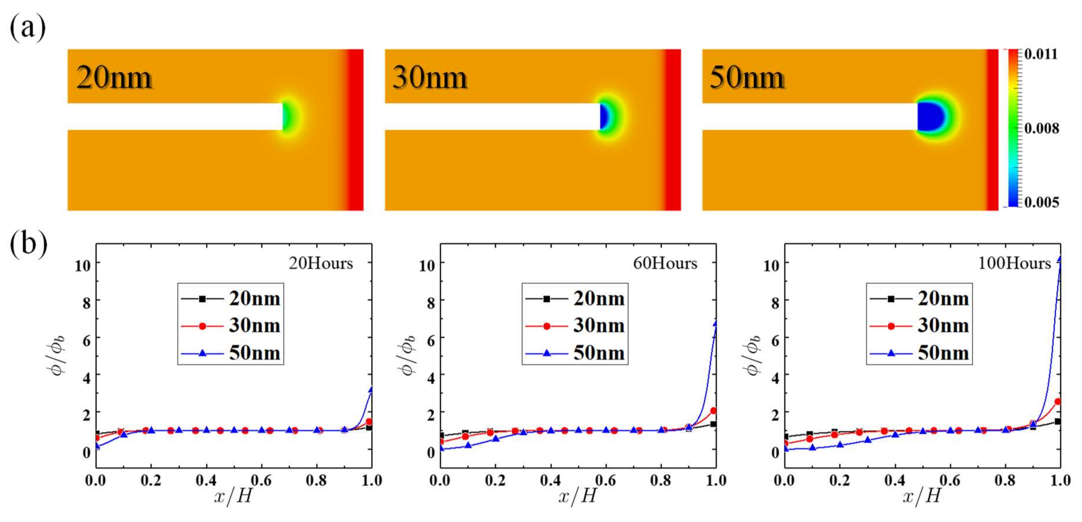
Figure 3 shows the effect of the nanoparticle type on the concentration distribution. Two types of particles are considered: and . Figure 3 indicates that the intensity of the nanoparticle accumulation is stronger for , which has a much higher density (see Table 2). According to Equations (14) and (15), the term representing the particle migration (due to gravity) is linearly proportional to the particle density. Figure 4 shows the effect of the nanoparticle size on the concentration distribution. As Equations (14) and (15) show, the particle flux due to gravity depends quadratically on the particle radius. Thus from Figure 4, we can see that as the particle size increases, the migration of the nanoparticles increases significantly. For a particle radius of 50 nm, a large region of low concentration near the end of the inner pipe can be observed, where the concentration is close to 0, see Figure 4a,b. Figure 5 shows the time evolution of particle accumulation, , with different nanoparticle sizes and types. The figures indicate that as the particle size or the density increases, increases; the effect of the nanoparticle size is more significant.
4.1.2. Effects of Particle Concentration and Ground Temperature
Figure 6a shows the effect of the ground temperature. As the ground temperature increases, the particle accumulation decreases a little, perhaps due to the increasing of the Brownian motion intensity (see Equations (9) and (10)). Figure 6b shows the effect of the nanoparticle bulk concentration. As the bulk concentration increases, the particle accumulation decreases a little, perhaps due to the increasing of the viscosity of the nanofluid. Overall, in the range of the parameters studied here, the effects of the nanoparticle concentration and the ground temperature on the concentration distribution are not significant. The particle concentration can increase the thermal conductivity of the nanofluids. On the other hand, temperature does directly affect the nanoparticle concentration through changing the intensity of the Brownian motion.
4.1.3. Effects of Inclined Angle of Pipes
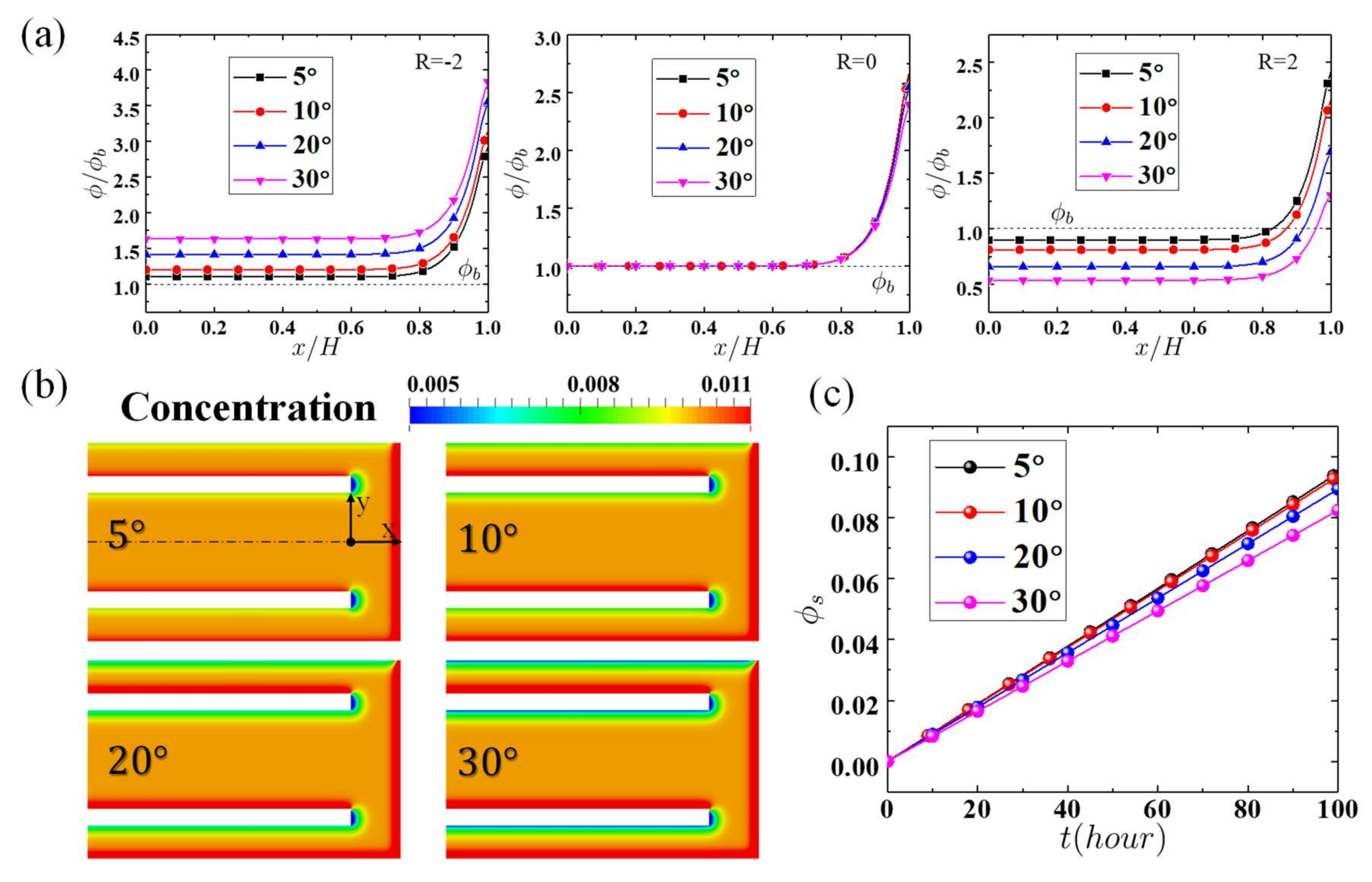
It has been shown that a slight tilt of the boreholes can substantially improve the performance of the geothermal heat exchanger [66]. Figure 7 shows the effect of the angle () between the pipes and the direction of gravity. When the pipe is vertical, . In the current geometry, the gravity is . For this situation, we cannot use the symmetry conditions; therefore, the problem (the mesh) is three dimensional. Figure 7a shows the time evolution of the concentration profiles along the X-direction at different radial positions −2, 0, and 2. At −2, due to gravity in the Y-direction, as the inclination angle increases, the concentration of the particles also increases. This is the opposite effect of the variation of the concentration profiles at 2 (see Figure 7b for more information); for 0, the variation is minimal. Figure 7c shows that as the inclination angle increases, the particles accumulated () near the bottom borehole region increase moderately.
4.2. Suspension Stability of the Nanofluids
In this section, the concentration field after 100 h of simulation is used as the initial condition to study the effect of the fluid flow on the accumulated nanoparticles. When the Reynolds number is higher than 2600, the flow is considered to become turbulent; when the Reynolds number is less than 2300, the flow is laminar. The Reynolds number is defined as , where and are the density and the viscosity based on the bulk volume fraction of the nanoparticles, respectively. We also define a dimensionless time: .
4.2.1. Effects of the Reynolds Number
Figure 8 shows the concentration profiles at different dimensionless times, , when the Reynolds number (Re) is 3686. As increases, the particle accumulation near the bottom decreases rapidly. At , the accumulation is almost negligible. Figure 9 shows the effect of the Reynolds number on the particle accumulation. Different Reynolds numbers can be achieved by changing the flow rate. For the same dimensionless time , as the Reynolds number increases, the particle accumulation decreases gradually. Figure 10 shows the time evolution of the nanoparticle concentration at radial positions R = 0 and R = 2 for different Reynolds numbers. Figure 11 shows the nanoparticle accumulation () as a function of time for different Reynolds numbers. Figure 10 and Figure 11 indicate, quantitatively, that the removal speed of the nanoparticle accumulation increases significantly as the Re changes from 921 to 3686.
4.2.2. Effects of the Pulsed Flow and the Bottom Borehole Geometry
We investigate two possible methods for improving the removal of the accumulated nanoparticles, namely (i) using a pulsed flow or (ii) changing the bottom borehole geometry. For the following simulations, the Reynolds number is assumed to be 921; therefore, the flow is laminar.
Figure 12 and Figure 13 show the effect of the pulsed flow on the nanoparticle accumulation. The pulsed flow is realized by applying a sinusoidal inlet velocity, , where is the frequency of the pulsed velocity and is the mean velocity. As expected, a pulsed flow enhances the disturbance of the flow and improves the removal of the particles accumulated; a higher pulse frequency () gives a better removal performance. From Figure 13b, the effect of the pulsed flow on the concentration profile at R = 2 is moderate, and the effect at R = 0 is very significant. Figure 14 shows that the removal of the accumulated particles can be improved by reducing the distance between the end of the inner pipe and the bottom borehole or rounding the corners of the bottom borehole.
It should be noted that following Buongiorno [34], in this paper, we have assumed that the migration of the nanoparticles can be induced by the Brownian motion, thermophoretic diffusion, gravity, and turbulent diffusivity, while the mechanism for the aggregation of nanoparticles has not been included. The suspension stability of the nanofluids is affected by , (a measure of the accumulated particles compared with the bulk concentration). In some situations, aggregation of the nanoparticles can occur, and as a result, the properties of the nanofluids change. Xuan et al. [67] simulated the aggregation process of the nanoparticles using the theory of Brownian motion and the diffusion-limited aggregation model; the simulations indicated that the nanoparticle aggregation reduces the thermal performance of the nanofluids, which agreed with their experimental measurements. Furthermore, although most nanofluids have been shown to have good suspension stability while also providing thermal enhancement in geothermal heat exchangers [2], the cost of using nanofluids should be considered. This could be an important economical concern because geothermal piles are usually very long, requiring a large amount of working fluid.
5. Conclusions
Nanofluids have been shown to increase the heat transfer coefficient in various applications, including geothermal heat exchangers. In this paper, we study the flow of nanofluids in a coaxial geothermal heat exchanger. The suspension is modeled as a non-linear, complex fluid; the nanoparticle migration is modeled by a particle flux model, which considers the effects of Brownian motion, gravity, turbulent eddy diffusivity, etc. Through numerical simulations, it is found that when nanofluid is static, particles tend to accumulate near the bottom borehole due to gravity; the nanoparticles sedimentation process usually takes several hours. It is also found that sedimentation is more noticeable for nanofluids with larger particle sizes or higher densities of nanoparticles. Furthermore, the variation of the inclination angle between the pipes and the direction of gravity also influences the sedimentation pattern. Once the flow/operation starts, the accumulated nanoparticles can be “washed” out within several minutes by fluid flowing at relatively high velocities, indicating good suspension stability of the nanofluids. With a higher Reynolds number, the accumulated nanoparticles can be cleaned much faster. We also find that a pulsed flow or an optimized geometry of the bottom borehole can potentially improve the stability of the suspension. It should be noted that the methods for improving the nanofluids’ suspension stability can be generalized for analyzing other types of solid particles existing in a heat exchanger.
Acknowledgments
Thanks for the funding support from the China Postdoctoral Science Foundation (No. 2017M611819, Xiao-hui Sun).
Author Contributions
Xiao-Hui Sun and Wei-Tao Wu did all the numerical simulations. Wei-Tao Wu and Mehrdad Massoudi derived all the equations. All the authors have provided substantial contributions to the manuscript preparation.
Conflicts of Interest
The authors declare no conflict of interest.
Nomenclature
| time | |
| particle response time | |
| Cartesian coordinates (m) | |
| pressure (Pa) | |
| Boltzmann constant (J/K) | |
| Nanoparticle radius (m) | |
| diameter of nanoparticles (m) | |
| thermal conductivity of nanofluid (W/(mK)) | |
| thermal conductivity of particles (W/(mK)) | |
| Schmidt number | |
| reference length scale (m) | |
| reference velocity (m/s) | |
| Reynolds number | |
| Froude number | |
| dimensionless pressure | |
| dimensionless number (Brownian motion) | |
| dimensionless number (turbulent) | |
| dimensionless number (gravity) | |
| inner diameter of inner pipe (m) | |
| outer diameter of inner pipe (m) | |
| inner diameter of outer pipe (m) | |
| Distance between pipe end and borehole bottom | |
| length of the heat exchanger (m) | |
| mean inlet velocity (m/s) | |
| pulse velocity (m/s) | |
| pulse frequency (Hz) | |
| position vector (m) | |
| velocity vector (m/s) | |
| stress tensor (Pa) | |
| body force vector (N/kg) | |
| particles flux (kg/(m2s)) | |
| particles flux (thermophoresis) (kg/(m2s)) | |
| particles flux (Brownian motion) (kg/(m2s)) | |
| particles flux (turbulent) (kg/(m2s)) | |
| particles flux (gravity) (kg/(m2s)) | |
| symmetric part of velocity gradient (s−1) | |
| dimensionless velocity vector | |
| gravity | |
| dimensionless position vector | |
| Greek symbols | |
| density of nanofluid (kg/m3) | |
| volume fraction of the base fluid | |
| volume fraction of nanoparticles | |
| density of base fluid (kg/m3) | |
| density of pure nanoparticles (kg/m3) | |
| dynamic viscosity of base fluid (Pa∙s) | |
| dynamic viscosity of nanofluid (Pa∙s) | |
| kinematic viscosity of nanofluid (m2/s) | |
| kinematic viscosity of base fluid (m2/s) | |
| turbulent eddy diffusivity (m2/s) | |
| temperature (K) | |
| dimensionless time | |
| density ratio | |
| inclined angle |
References
- Finger, J.; Blankenship, D. Handbook of best practices for geothermal drilling. Sandia Natl. Lab. Albuquerque 2010. [Google Scholar]
- Faizal, M.; Bouazza, A.; Singh, R.M. Heat transfer enhancement of geothermal energy piles. Renew. Sustain. Energy Rev. 2016, 57, 16–33. [Google Scholar] [CrossRef]
- Fridleifsson, I.B.; Bertani, R.; Huenges, E.; Lund, J.W.; Ragnarsson, A.; Rybach, L. The possible role and contribution of geothermal energy to the mitigation of climate change. In IPCC Scoping Meeting on Renewable Energy Sources, Proceedings, Luebeck, Germany; Pennsylvania State University: State College, PA, USA, 2008; Volume 20, pp. 59–80. [Google Scholar]
- Lund, J.W.; Boyd, T.L. Direct utilization of geothermal energy 2015 worldwide review. Geothermics 2016, 60, 66–93. [Google Scholar] [CrossRef]
- Lund, J.W. Direct utilization of geothermal energy. Energies 2010, 3, 1443–1471. [Google Scholar] [CrossRef]
- Wu, W.-T.; Aubry, N.; Antaki, J.F.; McKoy, M.L.; Massoudi, M. Heat Transfer in a Drilling Fluid with Geothermal Applications. Energies 2017, 10, 1349. [Google Scholar] [CrossRef]
- Østergaard, P.A.; Lund, H. A renewable energy system in Frederikshavn using low-temperature geothermal energy for district heating. Appl. Energy 2011, 88, 479–487. [Google Scholar] [CrossRef]
- Kwag, B.C.; Krarti, M. Performance of thermoactive foundations for commercial buildings. J. Sol. Energy Eng. 2013, 135, 40907. [Google Scholar] [CrossRef]
- Yavuzturk, C.; Spitler, J.D.; Rees, S.J. A transient two-dimensional finite volume model for the simulation of vertical U-tube ground heat exchangers. ASHRAE Trans. 1999, 105, 465. [Google Scholar]
- Marcotte, D.; Pasquier, P. On the estimation of thermal resistance in borehole thermal conductivity test. Renew. Energy 2008, 33, 2407–2415. [Google Scholar] [CrossRef]
- Ghasemi-Fare, O.; Basu, P. A practical heat transfer model for geothermal piles. Energy Build. 2013, 66, 470–479. [Google Scholar] [CrossRef]
- Ghasemi-Fare, O.; Basu, P. Predictive assessment of heat exchange performance of geothermal piles. Renew. Energy 2016, 86, 1178–1196. [Google Scholar] [CrossRef]
- Ozudogru, T.Y.; Olgun, C.G.; Senol, A. 3D numerical modeling of vertical geothermal heat exchangers. Geothermics 2014, 51, 312–324. [Google Scholar] [CrossRef]
- Ozudogru, T.Y.; Ghasemi-Fare, O.; Olgun, C.G.; Basu, P. Numerical modeling of vertical geothermal heat exchangers using finite difference and finite element techniques. Geotech. Geol. Eng. 2015, 33, 291–306. [Google Scholar] [CrossRef]
- Rees, S.J.; He, M. A three-dimensional numerical model of borehole heat exchanger heat transfer and fluid flow. Geothermics 2013, 46, 1–13. [Google Scholar] [CrossRef]
- Nalla, G.; Shook, G.M.; Mines, G.L.; Bloomfield, K.K. Parametric sensitivity study of operating and design variables in wellbore heat exchangers. Geothermics 2005, 34, 330–346. [Google Scholar] [CrossRef]
- Hu, J. An improved analytical model for vertical borehole ground heat exchanger with multiple-layer substrates and groundwater flow. Appl. Energy 2017, 202, 537–549. [Google Scholar] [CrossRef]
- Ghasemi-Fare, O.; Basu, P. Influences of ground saturation and thermal boundary condition on energy harvesting using geothermal piles. Energy Build. 2018, 165, 340–351. [Google Scholar] [CrossRef]
- Yan, H.B.; Zhang, Q.C.; Lu, T.J.; Kim, T. A lightweight X-type metallic lattice in single-phase forced convection. Int. J. Heat Mass Transf. 2015, 83, 273–283. [Google Scholar] [CrossRef]
- Yan, H.B.; Zhang, Q.C.; Lu, T.J. An X-type lattice cored ventilated brake disc with enhanced cooling performance. Int. J. Heat Mass Transf. 2015, 80, 458–468. [Google Scholar] [CrossRef]
- Li, Q.; Xuan, Y.; Wang, J. Investigation on convective heat transfer and flow features of nanofluids. J. Heat Transf. 2003, 125, 151–155. [Google Scholar]
- Lomascolo, M.; Colangelo, G.; Milanese, M.; de Risi, A. Review of heat transfer in nanofluids: conductive, convective and radiative experimental results. Renew. Sustain. Energy Rev. 2015, 43, 1182–1198. [Google Scholar] [CrossRef]
- Tang, W.; Hatami, M.; Zhou, J.; Jing, D. Natural convection heat transfer in a nanofluid-filled cavity with double sinusoidal wavy walls of various phase deviations. Int. J. Heat Mass Transf. 2017, 115, 430–440. [Google Scholar] [CrossRef]
- Jing, D.; Song, D. Optical properties of nanofluids considering particle size distribution: Experimental and theoretical investigations. Renew. Sustain. Energy Rev. 2017, 78, 452–465. [Google Scholar] [CrossRef]
- Choi, S.U.S. Enhancing thermal conductivity of fluids with nanoparticles. In Developments and Applications of Non-Newtonian Flows; ASME: New York, NY, USA, 1995; Volume 66, pp. 99–105. [Google Scholar]
- Eastman, J.A.; Choi, U.S.; Li, S.; Thompson, L.J.; Lee, S. Enhanced thermal conductivity through the development of nanofluids. In MRS Online Proceedings Library Archive; Cambridge University Press: Cambridge, UK, 1996; Volume 457, p. 3. [Google Scholar]
- Eastman, J.A.; Choi, S.U.S.; Li, S.; Yu, W.; Thompson, L.J. Anomalously increased effective thermal conductivities of ethylene glycol-based nanofluids containing copper nanoparticles. Appl. Phys. Lett. 2001, 78, 718–720. [Google Scholar] [CrossRef]
- Xuan, Y.; Li, Q. Heat transfer enhancement of nanofluids. Int. J. Heat Fluid Flow 2000, 21, 58–64. [Google Scholar] [CrossRef]
- Choi, S.U.S.; Zhang, Z.G.; Yu, W.; Lockwood, F.E.; Grulke, E.A. Anomalous thermal conductivity enhancement in nanotube suspensions. Appl. Phys. Lett. 2001, 79, 2252–2254. [Google Scholar] [CrossRef]
- Lotfi, R.; Rashidi, A.M.; Amrollahi, A. Experimental study on the heat transfer enhancement of MWNT-water nanofluid in a shell and tube heat exchanger. Int. Commun. Heat Mass Transf. 2012, 39, 108–111. [Google Scholar] [CrossRef]
- Ghozatloo, A.; Rashidi, A.; Shariaty-Niassar, M. Convective heat transfer enhancement of graphene nanofluids in shell and tube heat exchanger. Exp. Therm. Fluid Sci. 2014, 53, 136–141. [Google Scholar] [CrossRef]
- Daneshipour, M.; Rafee, R. Nanofluids as the circuit fluids of the geothermal borehole heat exchangers. Int. Commun. Heat Mass Transf. 2017, 81, 34–41. [Google Scholar] [CrossRef]
- Zhou, Z.; Wu, W.-T.; Massoudi, M. Fully developed flow of a drilling fluid between two rotating cylinders. Appl. Math. Comput. 2016, 281, 266–277. [Google Scholar] [CrossRef]
- Buongiorno, J. Convective Transport in Nanofluids. J. Heat Transf. 2006, 128, 240. [Google Scholar] [CrossRef]
- Phillips, R.J.; Armstrong, R.C.; Brown, R.A.; Graham, A.L.; Abbott, J.R. A constitutive equation for concentrated suspensions that accounts for shear-induced particle migration. Phys. Fluids A Fluid Dyn. 1992, 4, 30–40. [Google Scholar] [CrossRef]
- Wu, W.-T.; Massoudi, M.; Yan, H. Heat Transfer and Flow of Nanofluids in a Y-Type Intersection Channel with Multiple Pulsations: A Numerical Study. Energies 2017, 10, 492. [Google Scholar] [CrossRef]
- Massoudi, M. A note on the meaning of mixture viscosity using the classical continuum theories of mixtures. Int. J. Eng. Sci. 2008, 46, 677–689. [Google Scholar] [CrossRef]
- Phuoc, T.X.; Massoudi, M.; Chen, R.-H. Viscosity and thermal conductivity of nanofluids containing multi-walled carbon nanotubes stabilized by chitosan. Int. J. Therm. Sci. 2011, 50, 12–18. [Google Scholar] [CrossRef]
- Massoudi, M.; Vaidya, A. Analytical solutions to Stokes-type flows of inhomogeneous fluids. Appl. Math. Comput. 2012, 218, 6314–6329. [Google Scholar] [CrossRef]
- Tzou, D.Y. Thermal instability of nanofluids in natural convection. Int. J. Heat Mass Transf. 2008, 51, 2967–2979. [Google Scholar] [CrossRef]
- Wang, X.; Xu, X.; Choi, S.U. Thermal conductivity of nanoparticle-fluid mixture. J. Thermophys. Heat Transf. 1999, 13, 474–480. [Google Scholar] [CrossRef]
- Syam, S.L.; Singh, M.K.; Sousa, A.C.M. Investigation of thermal conductivity and viscosity of Fe3O4 nanofluid for heat transfer applications. Int. Commun. Heat Mass Transf. 2013, 44, 7–14. [Google Scholar] [CrossRef]
- Nguyen, C.T.; Desgranges, F.; Roy, G.; Galanis, N.; Maré, T.; Boucher, S.; Mintsa, H.A. Temperature and particle-size dependent viscosity data for water-based nanofluids–hysteresis phenomenon. Int. J. Heat Fluid Flow 2007, 28, 1492–1506. [Google Scholar] [CrossRef]
- Kwak, K.; Kim, C. Viscosity and thermal conductivity of copper oxide nanofluid dispersed in ethylene glycol. Korea-Aust. Rheol. J. 2005, 17, 35–40. [Google Scholar]
- He, Y.; Jin, Y.; Chen, H.; Ding, Y.; Cang, D.; Lu, H. Heat transfer and flow behaviour of aqueous suspensions of TiO2 nanoparticles (nanofluids) flowing upward through a vertical pipe. Int. J. Heat Mass Transf. 2007, 50, 2272–2281. [Google Scholar] [CrossRef]
- Subia, S.R.; Ingber, M.S.; Mondy, L.A.; Altobelli, S.A.; Graham, A.L. Modelling of concentrated suspensions using a continuum constitutive equation. J. Fluid Mech. 1998, 373, 193–219. [Google Scholar] [CrossRef]
- Wu, W.-T.; Massoudi, M. Heat Transfer and Dissipation Effects in the Flow of a Drilling Fluid. Fluids 2016, 1, 4. [Google Scholar] [CrossRef]
- Hsu, T.; Traykovski, P.A.; Kineke, G.C. On modeling boundary layer and gravity-driven fluid mud transport. J. Geophys. Res. Ocean. 2007, 112. [Google Scholar] [CrossRef]
- Drew, D.A. Production and dissipation of energy in the turbulent flow of a particle-fluid mixture, with some results on drag reduction. J. Appl. Mech. 1976, 43, 543–547. [Google Scholar] [CrossRef]
- Richardson, J.F.; Zaki, W.N. The sedimentation of a suspension of uniform spheres under conditions of viscous flow. Chem. Eng. Sci. 1954, 3, 65–73. [Google Scholar] [CrossRef]
- Acrivos, A.; Mauri, R.; Fan, X. Shear-induced resuspension in a Couette device. Int. J. Multiph. Flow 1993, 19, 797–802. [Google Scholar] [CrossRef]
- Mavromoustaki, A.; Bertozzi, A.L. Hyperbolic systems of conservation laws in gravity-driven, particle-laden thin-film flows. J. Eng. Math. 2014, 88, 29–48. [Google Scholar] [CrossRef]
- Abedi, M.; Jalali, M.A.; Maleki, M. Interfacial instabilities in sediment suspension flows. J. Fluid Mech. 2014, 758, 312–326. [Google Scholar] [CrossRef]
- Tominaga, Y.; Stathopoulos, T. Turbulent Schmidt numbers for CFD analysis with various types of flowfield. Atmos. Environ. 2007, 41, 8091–8099. [Google Scholar] [CrossRef]
- Rusche, H. Computational Fluid Dynamics of Dispersed Two-Phase Flows at High Phase Fractions; Imperial College London (University of London): London, UK, 2002; Volume 1. [Google Scholar]
- OpenCFD. OpenFOAM Programmer’s Guide Version 2.1.0; Free Software Foundation, Inc.: Boston, MA, USA, 2011. [Google Scholar]
- Wu, W.-T.; Yang, F.; Antaki, J.F.; Aubry, N.; Massoudi, M. Study of blood flow in several benchmark micro-channels using a two-fluid approach. Int. J. Eng. Sci. 2015, 95, 49–59. [Google Scholar] [CrossRef] [PubMed]
- Ubbink, O. Numerical Prediction of Two Fluid Systems with Sharp Interfaces. Ph.D. Thesis, University of London, London, UK, 1997. [Google Scholar]
- Kim, J. Multiphase CFD Analysis and Shape-Optimization of Blood-Contacting Medical Devices; Carnegie Mellon University: Pittsburgh, PA, USA, 2012. [Google Scholar]
- Jameson, A.; Schmidt, W.; Turkel, E. Numerical solution of the Euler equations by finite volume methods using Runge Kutta time stepping schemes. In Proceedings of the 14th Fluid and Plasma Dynamics Conference, Palo Alto, CA, USA, 23–25 June 1981; p. 1259. [Google Scholar]
- Fan, R.; Jiang, Y.; Yao, Y.; Shiming, D.; Ma, Z. A study on the performance of a geothermal heat exchanger under coupled heat conduction and groundwater advection. Energy 2007, 32, 2199–2209. [Google Scholar] [CrossRef]
- Job, V.M.; Gunakala, S.R. Mixed convection nanofluid flows through a grooved channel with internal heat generating solid cylinders in the presence of an applied magnetic field. Int. J. Heat Mass Transf. 2017, 107, 133–145. [Google Scholar] [CrossRef]
- Selimefendigil, F.; Öztop, H.F. Pulsating nanofluids jet impingement cooling of a heated horizontal surface. Int. J. Heat Mass Transf. 2014, 69, 54–65. [Google Scholar] [CrossRef]
- Barbés, B.; Páramo, R.; Blanco, E.; Pastoriza-Gallego, M.J.; Piñeiro, M.M.; Legido, J.L.; Casanova, C. Thermal conductivity and specific heat capacity measurements of Al2O3 nanofluids. J. Therm. Anal. Calorim. 2013, 111, 1615–1625. [Google Scholar] [CrossRef]
- Li, Y.; Yan, H.; Massoudi, M.; Wu, W.-T. Effects of Anisotropic Thermal Conductivity and Lorentz Force on the Flow and Heat Transfer of a Ferro-Nanofluid in a Magnetic Field. Energies 2017, 10, 1065. [Google Scholar] [CrossRef]
- Marcotte, D.; Pasquier, P. The effect of borehole inclination on fluid and ground temperature for GLHE systems. Geothermics 2009, 38, 392–398. [Google Scholar] [CrossRef]
- Xuan, Y.; Li, Q.; Hu, W. Aggregation structure and thermal conductivity of nanofluids. AIChE J. 2003, 49, 1038–1043. [Google Scholar] [CrossRef]
Figure 1.
Schematic of the coaxial geothermal heat exchanger.

Figure 2.
(a) Time evolution of the concentration profiles along the X-direction at different radial (Y) positions, R = 0, 1.167, and 2. (b) The concentration field near the borehole bottom at different times. (c) Nanoparticle accumulation, , as a function of time.
Figure 2.
(a) Time evolution of the concentration profiles along the X-direction at different radial (Y) positions, R = 0, 1.167, and 2. (b) The concentration field near the borehole bottom at different times. (c) Nanoparticle accumulation, , as a function of time.

Figure 3.
(a) Nanoparticle concentration fields with different types of nanoparticles after 100 h of simulation. (b) Time evolution of the concentration profiles along the X-direction with different types of nanoparticles at radial positions R = 0 (left) and 1.167 (right).
Figure 3.
(a) Nanoparticle concentration fields with different types of nanoparticles after 100 h of simulation. (b) Time evolution of the concentration profiles along the X-direction with different types of nanoparticles at radial positions R = 0 (left) and 1.167 (right).

Figure 4.
(a) Nanoparticle concentration fields with different sizes of nanoparticles after 100 h of simulation. (b) Nanoparticle profiles along the X-direction with different sizes of nanoparticles at radial position R = 1.167 and different times.
Figure 4.
(a) Nanoparticle concentration fields with different sizes of nanoparticles after 100 h of simulation. (b) Nanoparticle profiles along the X-direction with different sizes of nanoparticles at radial position R = 1.167 and different times.

Figure 5.
Effect of the nanoparticle size and type on nanoparticle accumulation, . (a) and (b) nanoparticle accumulation () as a function of time for different sizes.
Figure 5.
Effect of the nanoparticle size and type on nanoparticle accumulation, . (a) and (b) nanoparticle accumulation () as a function of time for different sizes.

Figure 6.
Effects of (a) the ground temperature and (b) the bulk nanoparticle concentration on the nanoparticle concentration profile along the X-direction at radial position R = 1.167 for different times.
Figure 6.
Effects of (a) the ground temperature and (b) the bulk nanoparticle concentration on the nanoparticle concentration profile along the X-direction at radial position R = 1.167 for different times.

Figure 7.
(a) Nanoparticle profiles along the X-direction at R = −2 (left), R = 0 (middle), and R = 2 (right) for different angles of inclination after 100 h of simulation. (b) Nanoparticle concentration field (x-y slice) for different angles of inclination after 100 h of simulation. (c) Nanoparticle accumulation () as a function of time with different angles.

Figure 8.
Nanoparticle concentration field near the bottom borehole at different dimensionless time, . The Reynolds number is 3686.
Figure 8.
Nanoparticle concentration field near the bottom borehole at different dimensionless time, . The Reynolds number is 3686.

Figure 9.
Nanoparticle concentration field at for different Reynolds numbers (Re).

Figure 10.
Time evolution of the nanoparticle concentration profiles for different Reynolds numbers. The profiles are plotted along the X-direction at radial positions (a) R = 0 and (b) R = 2.
Figure 10.
Time evolution of the nanoparticle concentration profiles for different Reynolds numbers. The profiles are plotted along the X-direction at radial positions (a) R = 0 and (b) R = 2.

Figure 11.
Nanoparticle accumulation () as a function of time for different Reynolds numbers.

Figure 12.
Nanoparticle concentration field for different pulse frequencies at 25 and 150.

Figure 13.
(a) Effect of the pulse frequency on the nanoparticle concentration profiles at R = 0. (b) Nanoparticle accumulation () as a function of time for different pulse frequencies.
Figure 13.
(a) Effect of the pulse frequency on the nanoparticle concentration profiles at R = 0. (b) Nanoparticle accumulation () as a function of time for different pulse frequencies.

Figure 14.
Nanoparticle concentration field at different times for different bottom borehole geometries: (left) The distance between the end of the inner pipe and the bottom borehole is ; (middle) The distance between the end of the inner pipe and the bottom borehole is ; and (right) Rounded bottom with . The Reynolds number is 921.


Table 1.
Boundary conditions used in our numerical simulations.
| Boundary Type | Pressure | Velocity | Concentration |
|---|---|---|---|
| Wall | Fixed flux (0) | Fixed value | Fixed flux (0) |
| Inlet | Fixed value (0) | Fixed value | Fixed value (0) |
| Outlet | Fixed value (0) | Fixed flux (0) | Fixed flux (0) |
© 2018 by the authors. Licensee MDPI, Basel, Switzerland. This article is an open access article distributed under the terms and conditions of the Creative Commons Attribution (CC BY) license (http://creativecommons.org/licenses/by/4.0/).
Share and Cite
MDPI and ACS Style
Sun, X.-H.; Yan, H.; Massoudi, M.; Chen, Z.-H.; Wu, W.-T. Numerical Simulation of Nanofluid Suspensions in a Geothermal Heat Exchanger. Energies 2018, 11, 919. https://0-doi-org.brum.beds.ac.uk/10.3390/en11040919
AMA Style
Sun X-H, Yan H, Massoudi M, Chen Z-H, Wu W-T. Numerical Simulation of Nanofluid Suspensions in a Geothermal Heat Exchanger. Energies. 2018; 11(4):919. https://0-doi-org.brum.beds.ac.uk/10.3390/en11040919
Chicago/Turabian StyleSun, Xiao-Hui, Hongbin Yan, Mehrdad Massoudi, Zhi-Hua Chen, and Wei-Tao Wu. 2018. "Numerical Simulation of Nanofluid Suspensions in a Geothermal Heat Exchanger" Energies 11, no. 4: 919. https://0-doi-org.brum.beds.ac.uk/10.3390/en11040919
Note that from the first issue of 2016, this journal uses article numbers instead of page numbers. See further details here.