A Practical Guide to Gaussian Process Regression for Energy Measurement and Verification within the Bayesian Framework

Department of Engineering Sciences, University of the Free State, P.O. Box 339, Bloemfontein 9300, South Africa
*
Author to whom correspondence should be addressed.
Energies 2018, 11(4), 935; https://0-doi-org.brum.beds.ac.uk/10.3390/en11040935
Submission received: 25 January 2018
/
Revised: 29 March 2018
/
Accepted: 4 April 2018
/
Published: 14 April 2018
(This article belongs to the Special Issue Bayesian Building Energy Modeling)
Abstract
:Measurement and Verification (M&V) aims to quantify savings achieved as part of energy efficiency and energy management projects. M&V depends heavily on metered energy data, modelling parameters and uncertainties that govern the energy system under consideration. M&V therefore requires a stringent handle on the inherent uncertainties in the calculated savings. The Bayesian framework of data analysis in the form of non-parametric, nonlinear Gaussian Process (GP) regression provides a mechanism by which these uncertainties can be quantified thoroughly, and is therefore an attractive alternative to the more traditional frequentist approach. It is important to select appropriate kernels to construct the prior when performing GP regression. This paper aims to construct a guideline for a practical GP regression within the energy M&V framework. It does not attempt to quantify energy losses or savings, but rather presents a case study that could act as a road map for energy managers and M&V professionals to apply the GP regression as a Bayesian alternative to base-line adjustment. Special attention will be given to the selection of appropriate kernels for the application of baseline adjustment and energy savings quantification in a model-independent manner.
1. Introduction
Energy saving measures (ESMs) usually aim to lower greenhouse gas (GHG) emissions in an attempt to mitigate climate change [1,2]. Energy efficiency also offers significant opportunities to lower the large financial costs associated with the use of fossil fuels [3].
In order to accurately quantify energy savings, accurate measurements and agreed upon methodologies are needed. Various Measurement and Verification (M&V) guidelines, such as The International Performance Measurement and Verification Protocol (IPMVP, see [3]), serve as industry-standards for energy M&V [1]. Better M&V generally results in higher savings with an increased level of confidence, thereby encouraging investment in energy efficiency and renewable energy projects [3]. Accurate quantification of savings is also important when considering tax-based incentives [1]. A very important factor to consider when interpreting savings is the inherent uncertainty in the data. Hamer et al. [1] reports that M&V calculations typically deviate from the actual observed savings by 10%. The IPMVP highlights instrumentation and modelling error as two quantifiable sources of inaccuracy in the M&V process and stresses the importance of reporting possible savings as well as a well-defined uncertainty [3].
Carstens et al. [4] rightfully points out that the traditional frequentist approach for obtaining well-defined uncertainty can lead to misinterpretation of the uncertainty it conveys. This creates an opportunity for the use of nonlinear Gaussian Process (GP) regression within the Bayesian paradigm for quantifying uncertainties in the M&V process [5]. The probabilistic nature of Bayesian models means that uncertainty is well defined [4]. GP regression can therefore provide true confidence in the calculated savings of energy efficiency projects and in that way provide more bankable figures and reliable retrofit campaigns.
Determining the parameters that govern typical energy demand models could become time-consuming and expensive. This is especially true for energy systems that have high sensitivity to complex external parameters and usage patterns (see [6] for examples). GP regression, on the other hand, yields more robust predictions of energy use [7]. The predictive power of GP regression will be illustrated in a forthcoming paper, as this paper mainly communicates a case study of energy management M&V that could benefit from GP regression.
Another attractive property of the Bayesian paradigm is that little knowledge of the underlying energy model is necessary, thus reducing the induced error associated with the model [8]. The Bayesian paradigm allows the data to “speak for itself”, thus largely eliminating the modelling error in M&V [4,9].
To explain the GP without the use of technical statistical jargon, this paper makes use of the fundamental concept of inference. Inference, as used in this paper, refers to the concept of learning from a time-stamped data set that describes a specific energy driver associated with a building. To infer a mathematical structure that describes the dependencies and relationships between individual observations without prior knowledge of the governing parameters is the main purpose of the Bayes and GP paradigm. The inferred mathematical structure that describes the relationships between instances in the time series data set can be used to derive a set of evidence-based rules that could be useful for predictive purposes. M&V describes the process of determining the savings generated by an energy intervention and requires well-known uncertainty. The uncertainties associated with measured data (also called noisy evidence) are propagated forward by the GP and the GP thus generates a framework to predict system outputs using evidence in a probabilistic manner. The reader is referred to Reddy and Claridge [8] for the technical details of uncertainty propagation in GP algorithms.
The Bayesian paradigm is mathematically formulated by Bayes’ Theorem:
Theorem 1.
.
In Theorem 1, denotes probability, while | indicates conditional probability. When applied in the field of M&V, Theorem 1 provides the probability of savings given the measurements, . The uncertainty in savings is captured by , the uncertainty in measurement is given by , while the uncertainty in measurement given the savings is incorporated by . The fact that is well defined by Theorem 1 supports what is fundamentally required for M&V.
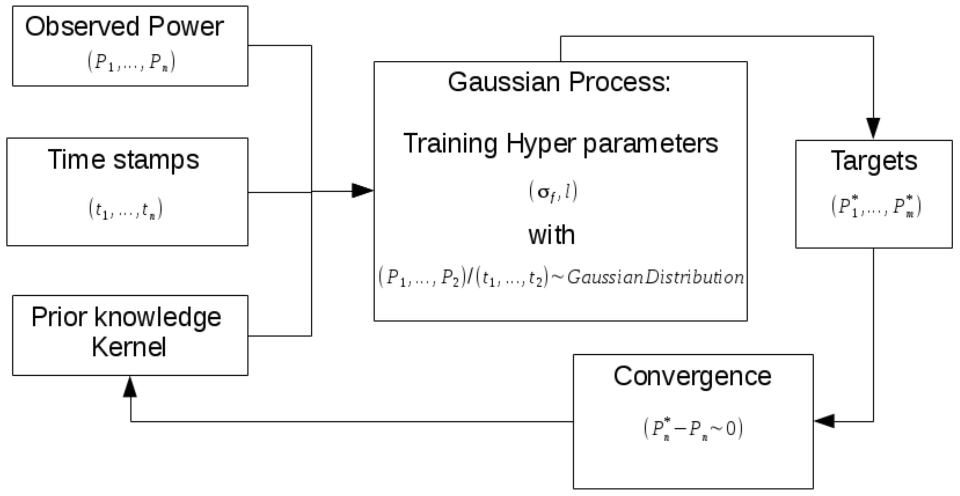
The GP is part of the Bayesian paradigm since both rely on the construction of a prior distribution. Rather than allocating a specific energy model (or function) to the data regression, the GP regresses data in a non-parametric, yet certain, way (see Rasmussen and Williams [10], Carstens et al. [4] and Figure 1).
Figure 1 illustrates the structure of a typical GP algorithm for use in energy savings quantification.
GP is a supervised machine learning regime that requires the refinement of two statistical hyper-parameters: the variance () and step length (l). This is done by specifying a prior (based on a carefully chosen kernel) and then refining the hyper-parameters iteratively based on a training set, in order to generate the posterior. If the kernel is chosen wisely, convergence will ensue and predictions (with well-defined uncertainty) can be made about the behaviour of the energy system and its parameters. Refer to the classical text Gaussian Processes for Machine Learning by Rasmussen and Williams [10] for an in-depth study of Gaussian Processes.
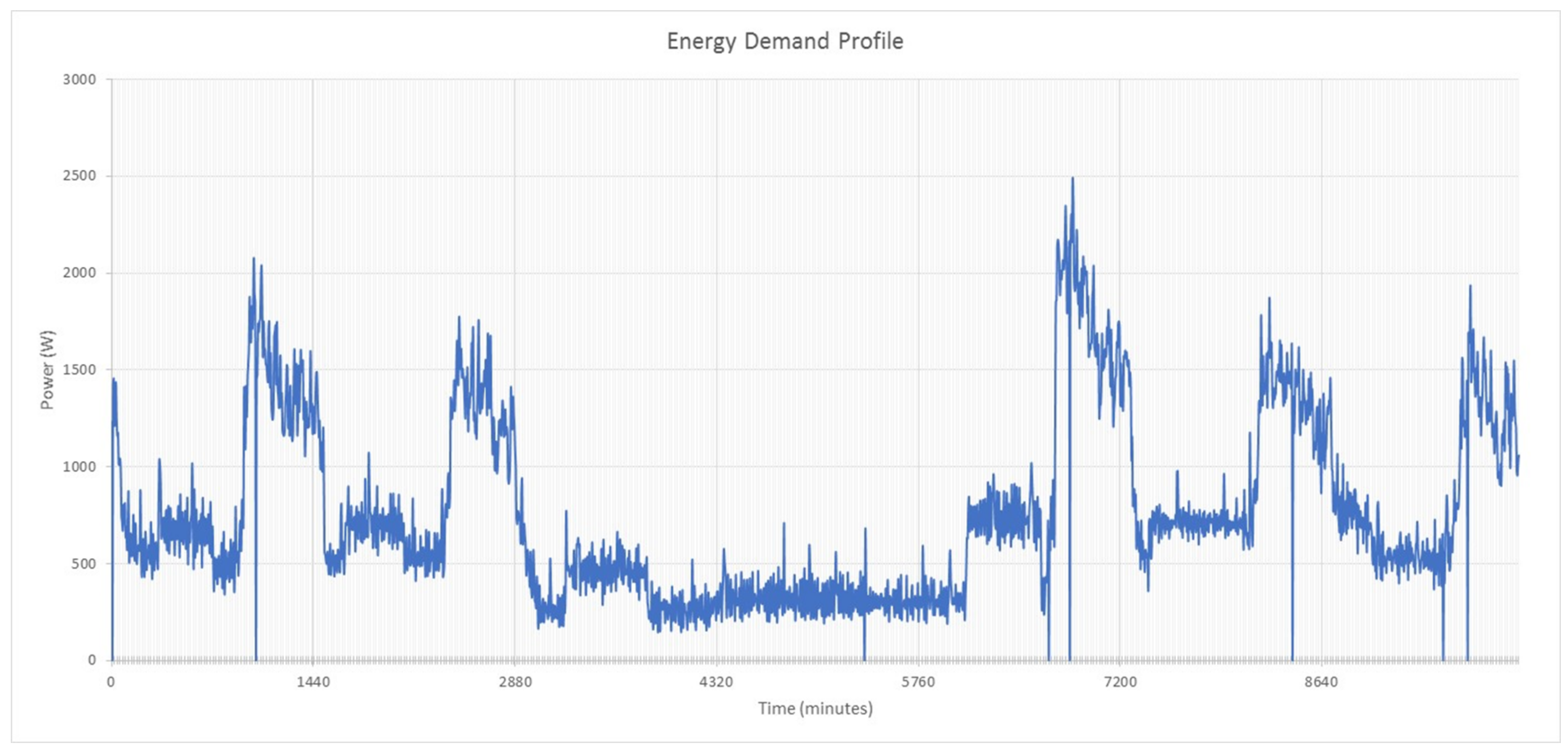
To conclude this introduction, the reader is referred to Figure 2, which illustrates a complex demand profile at an academic department for a period of one week. This academic department consists of various energy-consuming entities, such as offices, laboratories, lecture halls and kitchen facilities—all containing heating, ventilation and air conditioning (HVAC) systems. These entities are governed mostly by a human–building interaction, which automatically gives rise to periodicities in the demand profile (see Figure 2) [11]. Compiling an energy model to describe and predict this observed demand profile is difficult and can lead to misunderstandings and uncertainties. In this context, it would be useful to have the demand data construct its own model—to let the data ’speak for itself’. Notice also the following prominent signatures present in the demand profile (illustrated in Figure 2):
- Small, irregular variations,
- Day/night variations, with energy usage peaking approximately at midday,
- Low energy usage during weekends (between 2880 min and 5800 min in Figure 2).
Because of these apparent periodicities in the energy demand profile, together with the fact that the energy model is mostly unknown, the GP is an attractive modelling tool and will be able to regress the profile trend for the purpose of investigating possible forecasting and quantification of savings. This regression capabilitiy of the GP is a powerful tool for analysing the impact of energy related retrofits. The possibility also exists that the GP will statistically highlight previously unnoticed length scales that govern the energy model.
Referring to Figure 2, constructing the energy model that governs the observed profile can be done recursively: subtracting contributing factors (such as occupant behaviour and schedules) from the measured demand to reveal smaller and smaller model residuals until a random noise structure is achieved. However, interconnections of certain model parameters with each other and the global trend of the profile can prove difficult to find using this iterative process. What would be considered to be mere random noise could in fact be contributing energy factors. Thus, the GP provides a more holistic, more certain, method of finding the energy model that describes the system. This model is then ideal for the purpose of forecasting and saving quantification as induced by an energy management intervention or wastage anomaly.
This example serves to illustrate that GP regression can make a significant contribution within the energy M&V environment [12]. Due to the cyclic variations, a kernel can be chosen that adheres to the day/night cycle, or daily usage patterns.
The benefits of an alternative regression model becomes evident in the example above (see Figure 2), where the process of decomposing the demand profile to isolate primary parameters governing the system, is cumbersome and expensive. The usage patterns and governing dynamic systems are embedded in the energy model and warrant further exploration.
For further reference on the use of the GP modelling framework to determine energy savings, see Heo and Zavala [13].
Article Layout
The article is arranged as follows: Section 2 illustrates the usefulness of the GP regression by presenting a case study of the possible benefits that could be achieved by energy management interventions or energy wastage mitigation. In Section 3, practical guidelines are provided for setting up the GP, with special attention given to choosing the kernel based on the available data. The accommodation of model and measurement uncertainties are also discussed. Attention is given to the particular data set used in this study. The use of performance monitoring mechanisms for GP regression is also discussed. Section 4 outlines the experimental procedure followed to obtain the HVAC energy management case study (as presented in Section 2). Finally, Section 5 concludes with investigating the possibilities of applying GP analysis to demand management, incorporation of renewable energy alternatives, as well as its application to a green building index.
2. Results
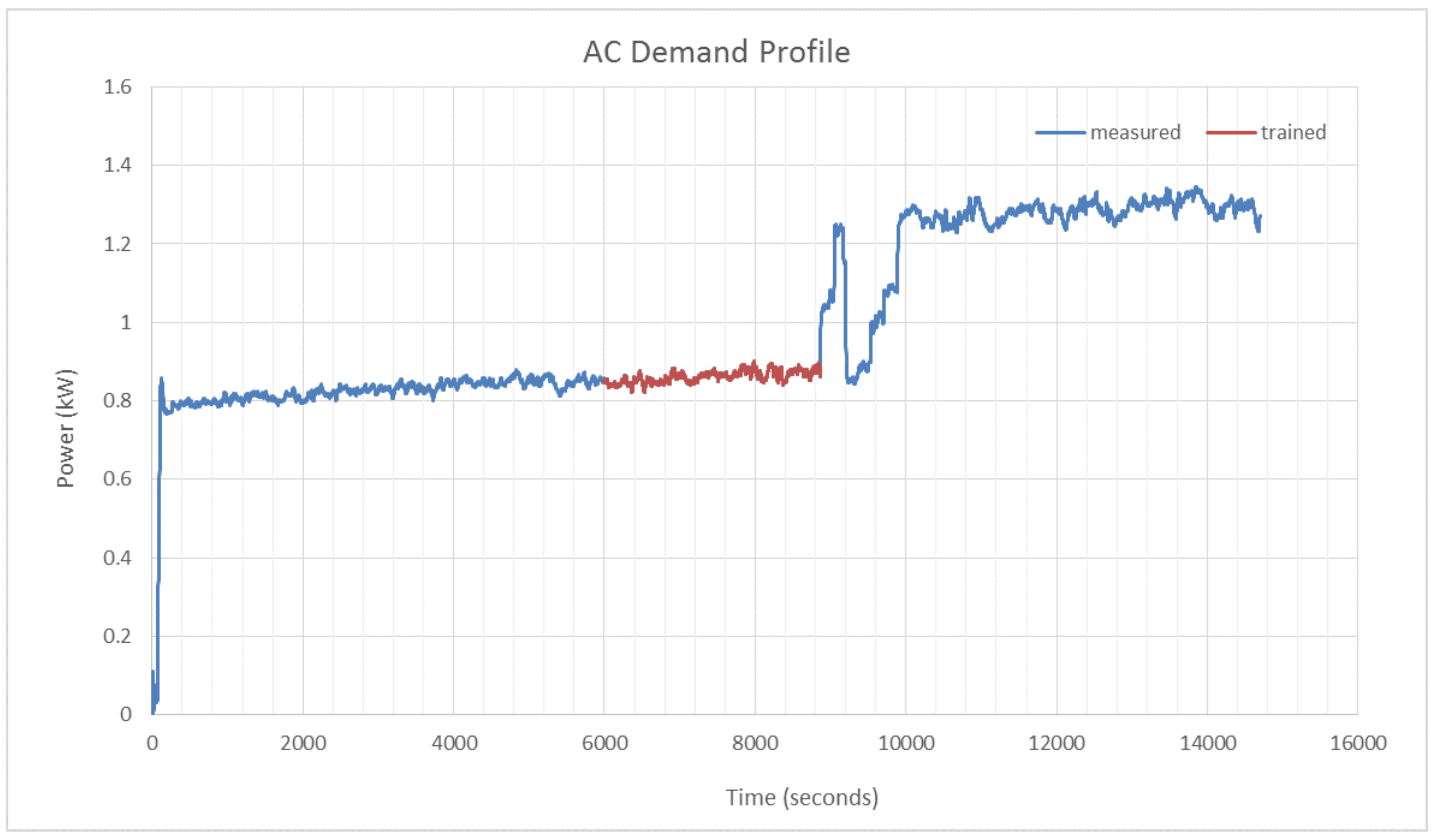
By making use of a GP regression, the energy model of an air conditioning (AC) system was inferred [14] (see Figure 3). A training set defined between s and s was used to train the hyper-parameters. After training, these optimized parameters were found to be kW and s. These parameter values are significant since they correspond to the mean set-point power consumption and possibly the switching time scales of the AC controller, respectively. Notice that the GP converged on hyper-parameters that can be linked directly to the physical nature of the energy system under consideration.
Figure 3 illustrates two distinct regions: a region of steadily increasing energy usage (from to s), which fluctuates slightly and periodically, and a region where the energy use rises abruptly (from s onwards). The sudden rise in energy use is due to an opened office door that resulted in an influx of hot air. A forecast energy demand from the point of the hot air influx, therefore, will be an estimate of what the energy use would have been if the door had not been opened. This corresponds to the principle of baseline adjustment, as part of M&V. By calculating the difference between the real and predicted energy use, an estimate of the energy wastage due to the open door can be calculated (with well-defined uncertainty).
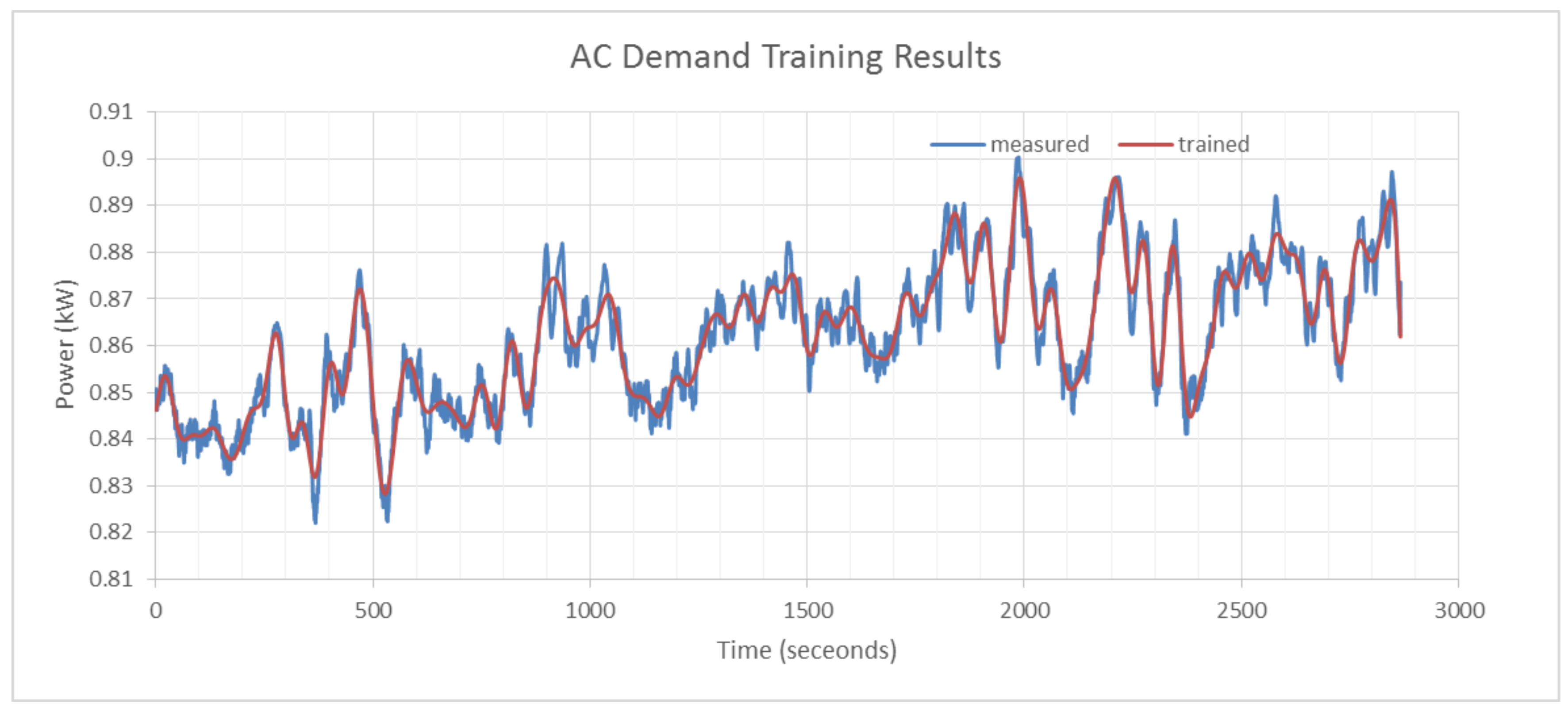
Figure 4 illustrates the training set (measured) and subsequent trained model of the AC demand profile. Figure 4 therefore corresponds to the training section ( s to s) in Figure 3.
Figure 4 clearly illustrates the precision with which an energy demand profile can be trained using GP.
The quantitative forecasting of energy demand for the purposes of quantifying energy savings falls outside the scope of this specific case study and will be dealt with in detail in a forthcoming paper.
3. Discussion
The GP process can be structured into key steps that are closely related to the data structure and requirements as set out by the energy manager.
3.1. Setting up the Gaussian Process
Choosing the Kernel
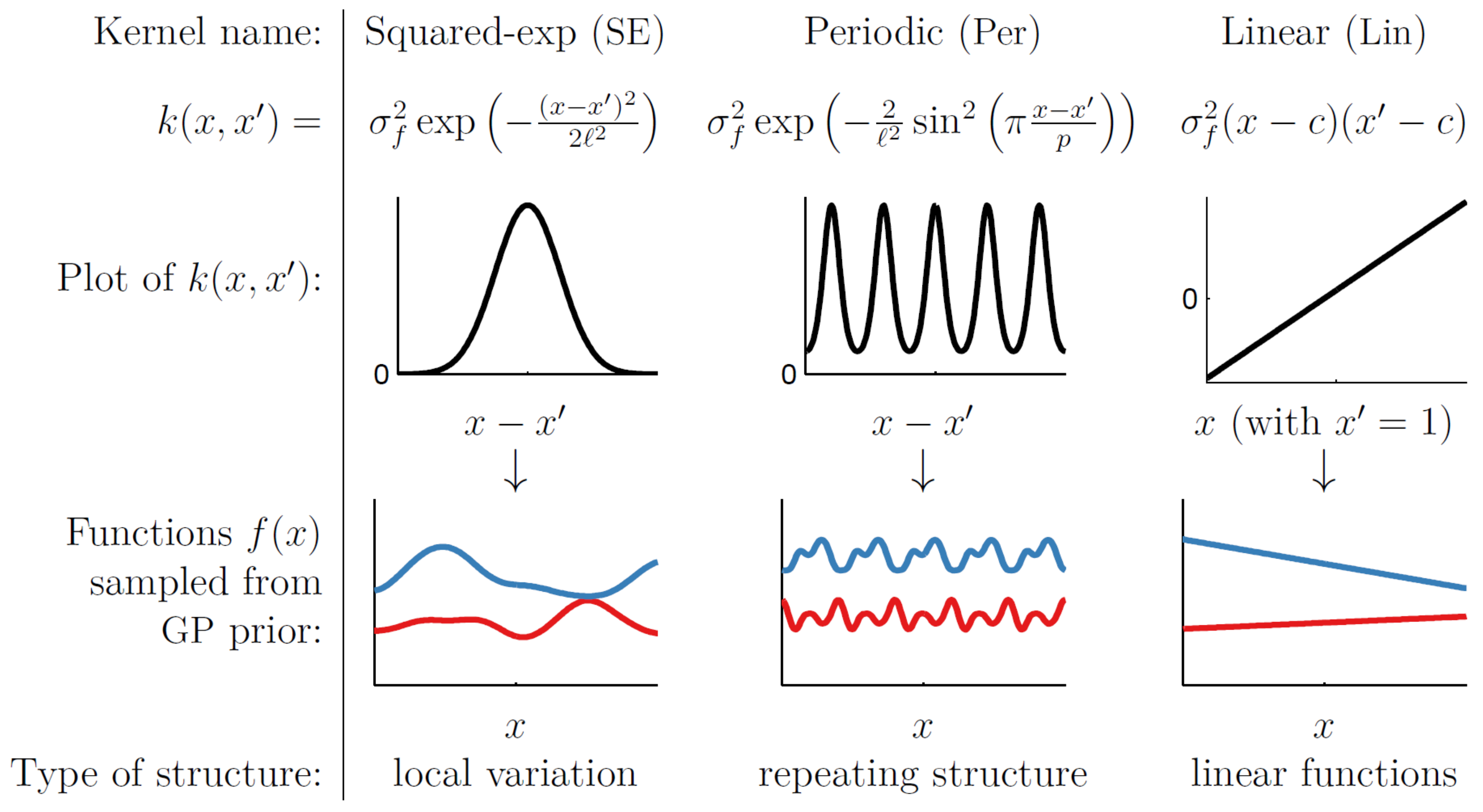
A kernel is also known as a covariance function of two inputs, and specifies the “similarity” between two objects [15]. Table 1 is a summary of some common kernels that can be used to perform GP regression on energy data.
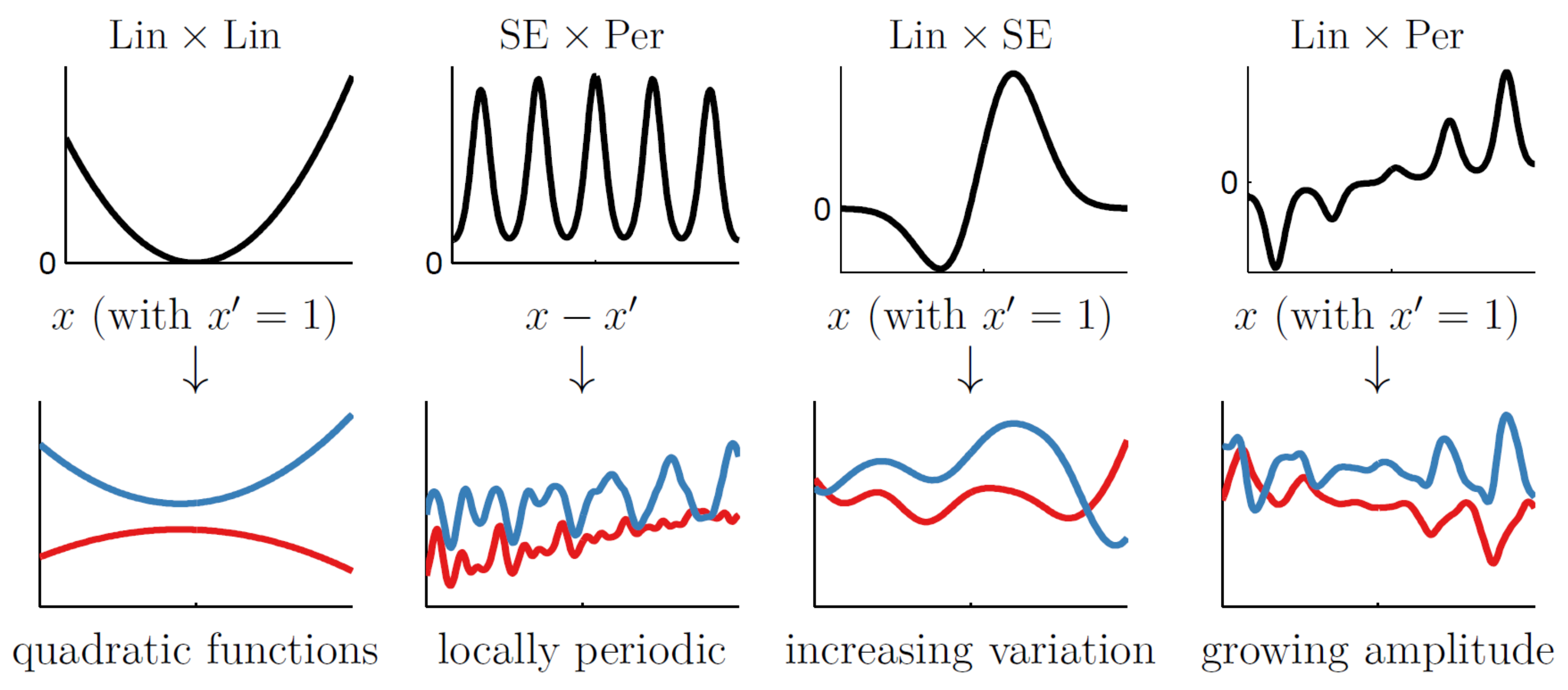
Figure 5 and Figure 6 illustrate some of the structures that are expressible by different kernels. Note that characteristic patterns in the data can be captured by specific kernels, as indicated in Figure 5.
Kernels can also be multi-dimensional, providing for the possibility of incorporating interconnected energy model parameters. The commonly used squared-exponential (SE) kernel
will give a larger value if x and are closer to each other, signifying a stronger similarity between x and . Kernels as covariance functions can therefore be used as a compact way of specifying the prior when setting up a GP regression. The amount of uncertianty in the GP regression will depend on the prior [16]. By inspecting a dataset, or by making an informed guess about the nature of the model to be regressed, appropriate custom kernels can be constructed by combining fundamental kernels. Each kernel used in the combination corresponds to a different assumption about the model under consideration [15]. Local variation will be represented by the squared-exponential kernel, repeating structure by a periodic kernel, and linearities by a linear kernel, and so forth [15]. Referring back to Figure 2, the weekly and daily variations could be modelled by periodic kernels multiplied by a squared exponential kernel. Multiplying the periodic kernel with the squared exponential kernel gives the periodic kernel some form of locality. The daily trend sits on top of the weekly trend and should therefore be transformed to a local trend. The small variations could be modelled with a squared exponential kernel with short length scale. Equation (2) is an example of such a kernel:
The parameters in the above custom kernel (Equation (2)) define the shape of the covariance function. They specify a distribution over the parameters of the implied model, and do not specify the function directly [15]. The length scale parameters, to , specify the width of the kernel and by doing so determine the smoothness of the functions in the model [15]. Different length scales are chosen based on observed or implied characteristics of the underlying model. In the case of the energy demand profile of Figure 2, a length scale in the order of minutes can be chosen to represent the small, irregular variations. A two-hour length scale can be used to represent the day/night variations and a length scale of seven days could be chosen to represent the trend of low energy use over weekends.
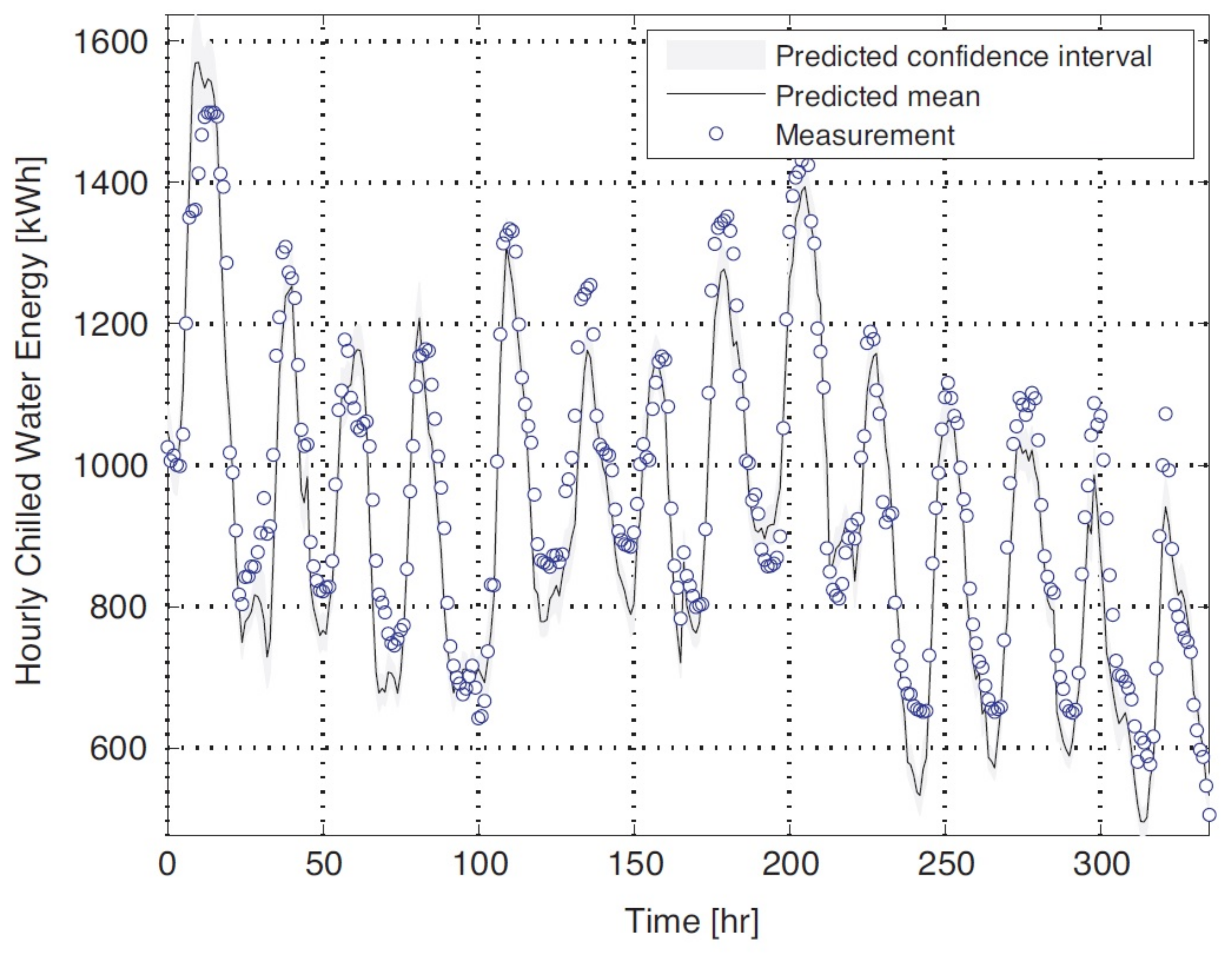
Figure 7 illustrates the predictive power of the GP [12]. The profile being predicted is that of hourly chilled water energy. Similar to the data fitted in Figure 3, small variations are present. Should the length scale of the GP be made larger, the confidence interval will degrade since the co-variance will have to consider more data points spanning longer time scales. Smaller variations in the data will therefore be lost.
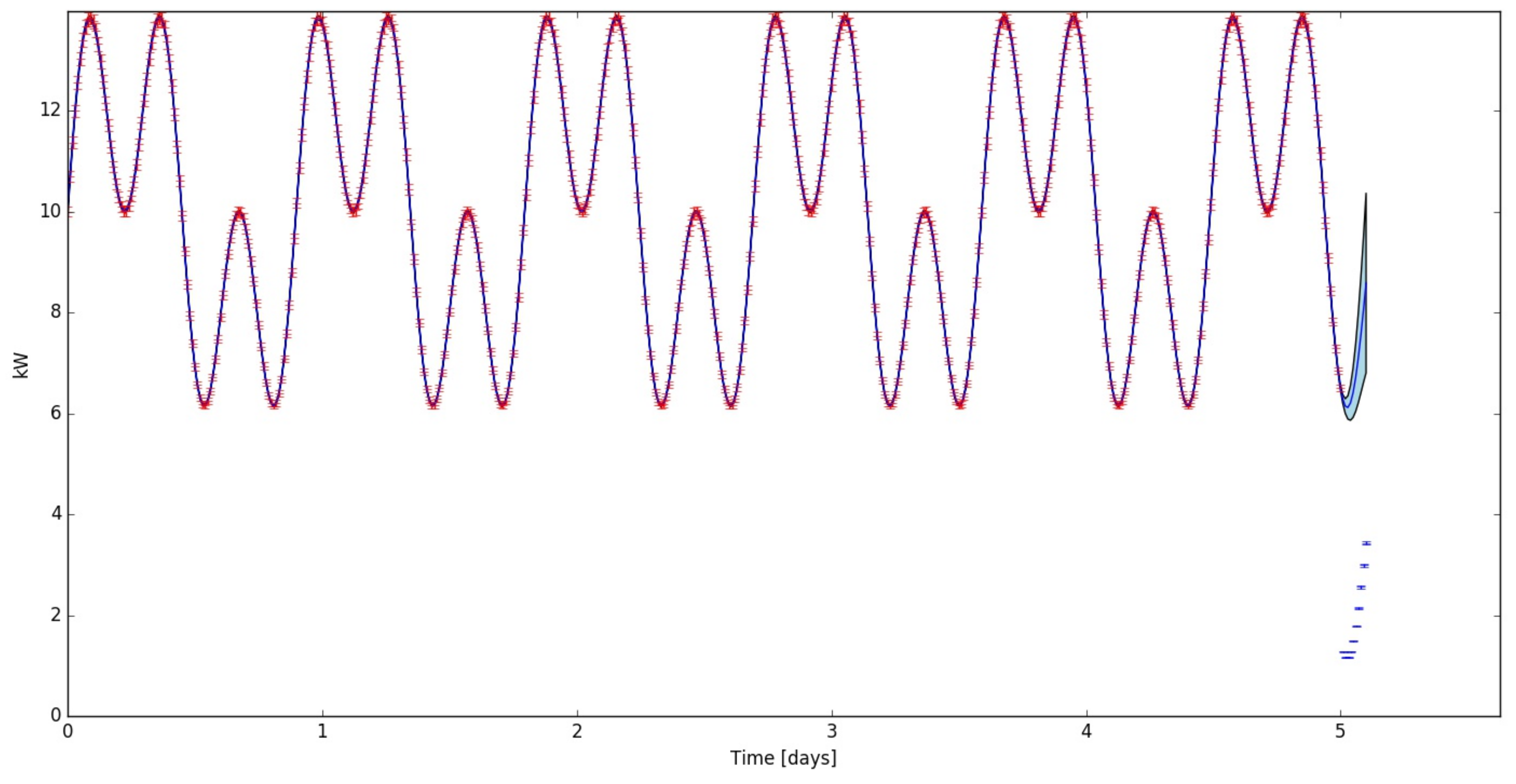
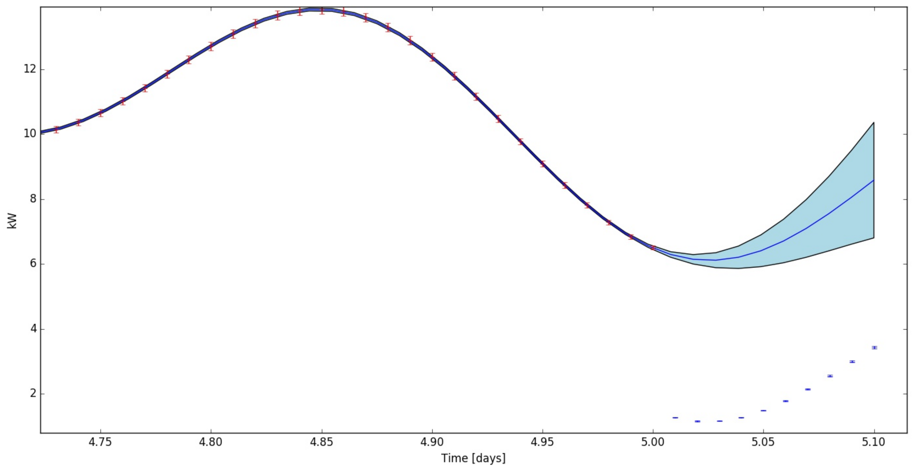
To further illustrate the usefulness of the GP as a prediction mechanism within the framework of M&V, the reader’s attention is drawn to Figure 8 and Figure 9. These figures illustrate a generic system with daily and inter-daily load variations over a period of 5.1 days. The system underwent an energy intervention at days, and the GP was used to predict the baseline from this point onwards in order to compare the predicted with the measured load. Since both the predicted and measured loads have associated errors (see Table 2), the savings are found as the difference between these two sets of data.
The energy intervention illustrated in Figure 8 reduced the load at days. Between days and days, the savings can be quantified by subtracting the real load (with blue error bars) from the predicted load (with error in shaded blue). The optimized hyperparameter for this GP was found to be .
More examples of GP prediction of steam and electricity consumption can be found in Yan et al. [17]. In this case, weekly variations are present and, if the GP length scale is set to one year, for example, the weekly and monthly variations will be ignored. This will degrade the confidence region.
3.2. Accommodating Uncertainties
The metering instrument used to create the energy usage dataset for the case study in Section 2 has an inherent uncertainty of . The GP treats the inputs to the training set (the pre-intervention energy usage data) not as point estimates, but as random points with known distribution (known mean and variance) [4,16]. This is referred to as probabilistic programming and is a powerful approach since it automatically allows for well-defined quantification of the uncertainties [4].
One of the benefits of the GP regression is therefore that uncertainty can be linked with predicted model outputs. For the case study presented in this paper, the model outputs will be kilowatt values together with a confidence interval (±kW). The mathematical machinery needed by the GP to cast the uncertainty in the output as a function of the uncertainty in the original measured data is outside the scope of this article, and the reader is referred to Rasmussen and Williams [10] for an in-depth analysis.
3.3. Monitoring Performance
It is valuable to know how well the GP regression fits the data within the training set. The coefficient of determination gives a quantitative measure of the goodness of fit. This method is, however, sensitive to the global pattern of the demand profile and appropriate utilization of other methods are therefore warranted [18]. The method of standardized mean squared error is based on the variance of the predicted values. If a predictive distribution is specified for every point in the target list, the negative log probability of the prediction that adheres to the model can be used [18].
Based on the standardized mean squared error, the conclusion can be made that the GP algorithm performs well for the AC demand profile presented in Section 2 since the algorithm converged: (see Figure 1).
The GP requires inversion and the determinant of the covariance matrix and could scale as in higher dimensional cases. More computational power is needed as the number of measurements increase and a numerical framework will be discussed in a future paper [19].
4. Instrumentation and Methods
A demand profile is obtained by measuring the energy consumption (in kW) of an office AC system for a set period of time during office hours. An energy wastage anomaly is simulated by deliberately allowing for the influx of hot air into the air conditioned space, and the post-intervention energy consumption is measured and recorded. The pre-intervention demand profile is used to train the GP. This training set is carefully chosen to represent a section of the demand profile just before the wastage anomaly, in order to enable a clear forecasting savings quantification opportunity. By comparing this forecast to the post-intervention measurement, the realised savings can be calculated. The energy savings can be translated to a monetary value to illustrate the economic impact of energy efficiency. This realisation forms part of the fundamental methodology for quantifying energy savings within the Bayesian paradigm.
5. Conclusions
The case study presented in this paper acts as an example of Bayesian alternatives (GP regression) for standard M&V analysis. It illustrates the non-parametric regression of time series data, given measurements and initial probabilities. The applicability and usefulness of non-parametric GP regression for the proper quantification of uncertainties within the M&V realm was illustrated.
This paper can be used as a road map by energy managers and M&V professionals to give guidance in identifying the point of intervention/wastage, selecting the prior training set (before the energy intervention/wastage), and forecasting of the energy system as if no energy intervention/wastage ever occurred (also known as base-line adjustment). However, the actual forecasting and energy loss quantification are not addressed in this paper and will be analysed in future.
The process of forecasting the training set, from before the point of intervention/wastage towards the point of the energy saving query, while taking into account the propagation of uncertainty in data, allows the calculation of the savings realised by energy saving interventions. Once the forecasted energy system (based on training data without the energy interventions/wastage) is compared to actual measurements (taken after the intervention/wastage point), the actual savings can be calculated. The case study presented in this paper is intended to inspire further exploration of GP regression as a Bayesian alternative to M&V principles, specifically the process of base-line adjustment.
The predictive power of the GP regression could furthermore be applied to demand management, the analysis of ESMs, as well as the analysis of renewable alternatives in the field of green buildings and net-zero homes. Energy demand and supply forecasting, and subsequent energy management, is a powerful tool for improving the status of a building’s green building rating [20].
The M&V principles associated with ESMs can be made more reliable, thereby improving the efficiency of tax incentives, green building rating systems and energy management campaigns. The GP regression could also be used to predict solar energy potential (supply side). Predicting the availability of renewable energy resources is critical in a holistic energy management plan. Since the GP updates its belief-system every time new data (or evidence) is added, it can easily be incorporated into real-time monitoring and management protocols.
The paradigm shift achieved by using the Bayesian approach can deliver a more robust method of energy data regression, which can include multi-dimensional data measurements for the entire system (power consumption, water usage and waste management).
The use of the GP therefore extends beyond M&V into the broader energy management sector.
Future work will include the training of a GP regression with weekly load cycles that include the features of day/night variation and weekends, by constructing the appropriate kernel. This training will be followed by the prediction of the load cycle and will demonstrate the full predictive power of GP regression by comparison to actual data.
Acknowledgments
We acknowledge the financial support of the Manufacturing, Engineering and Related Services Sector Education and Training Authority (merSETA), as well as colleagues of the Engineering Sciences Department at the University of the Free State.
Author Contributions
Jacques Maritz and Foster Lubbe conceived and designed the experiments that led to measurements and modelling. Jacques Maritz, Foster Lubbe and Louis Lagrange contributed to writing, compiling and formatting the paper.
Conflicts of Interest
The authors declare no conflict of interest.
References
- Hamer, W.; Booysen, W.; Mathews, E. A Practical Approach to Managing Uncertainty in the Measurement and Verification of Energy Efficiency Savings. South Afr. J. Ind. Eng. 2017, 28, 128–146. [Google Scholar] [CrossRef]
- Carstens, H. A Bayesian Approach to Energy Monitoring Optimization. Ph.D. Thesis, University of Pretoria, Pretoria, South Africa, 2017. [Google Scholar]
- International Performance Measurement and Verification Protocol (IPMVP). Concepts and Options for Determining energy and Water Savings; Technical Report; International Performance Measurement and Verification Protocol (IPMVP): Washington, DC, USA, 2002.
- Carstens, H.; Xia, X.; Yadavalli, S. Bayesian Energy Measurement and Verification Analysis. Energies 2018, 11, 380. [Google Scholar] [CrossRef]
- Walter, T.; Price, P.N.; Sohn, M.D. Uncertainty estimation improves energy measurement and verification procedures. Appl. Energy 2014, 130, 230–236. [Google Scholar] [CrossRef]
- Blum, M.; Riedmiller, M. Electricity Demand Forecasting using Gaussian Processes. In Proceedings of the 15th AAAI Conference on Trading Agent Design and Analysis, Washington, DC, USA, 14–15 July 2013. [Google Scholar]
- Burkhart, M.C.; Heo, Y.; Zavala, V.M. Measurement and Verification of Building Systems Under Uncertain Data: A Gaussian Process Modeling Approach. Energy Build. 2014, 75, 189–198. [Google Scholar] [CrossRef]
- Reddy, T.A.; Claridge, D.E. Uncertainty of “Measured” Energy Savings from Statistical Baseline Models. HVAC&R Res. 2000, 6, 3–20. [Google Scholar]
- Neal, R. Bayesian Learning for Neural Networks; Springer Science & Business Media: Berlin/Heidelberg, Germany, 2012. [Google Scholar]
- Rasmussen, C.E.; Williams, C.K.I. Gaussian Processes for Machine Learning; MIT Press: Cambridge, MA, USA, 2006; Volume 14, pp. 69–106. [Google Scholar]
- Booth, A.; Choudhary, R.; Spiegelhalter, D. A hierarchical Bayesian framework for calibrating micro-level models with macro-level data. J. Build. Perform. Simul. 2013, 6, 293–318. [Google Scholar] [CrossRef]
- Heo, Y. Bayesian Calibration of Building Energy Models for Energy Retrofit Decision-Making under Uncertainty. Ph.D. Thesis, Georgia Institute of Technology, Atlanta, GA, USA, 2011. [Google Scholar]
- Heo, Y.; Zavala, V. Gaussian Process Modeling for Measurement and Verification of Building Energy Savings. Energy Build. 2012, 53, 7–18. [Google Scholar] [CrossRef]
- Seikel, M.; Clarkson, C.; Smith, M. Reconstruction of dark energy and expansion dynamics using Gaussian processes. J. Cosmol. Astropart. Phys. 2012, 6, 036. [Google Scholar] [CrossRef]
- Duvenaud, D.K. Automatic Model Construction with Gaussian Processes (Charper 1). Ph.D. Thesis, University of Cambridge, Cambridge, UK, 2014. [Google Scholar]
- Quiñonero-Candela, J. Learning with Uncertainty-Gaussian Processes and Relevance Vector Machines. Ph.D. Thesis, Technical University of Denmark, Copenhagen, Denmark, 2004. [Google Scholar]
- Yan, B.; Li, X.; Shi, W.; Zhang, X.; Malkawi, A. Forecasting Building Energy Demand under Uncertainty Using Gaussian Process Regression: Feature Selection, Baseline Prediction, Parametric Analysis and a Web-Based Tool. In Proceedings of the 15th IBPSA Conference, San Francisco, CA, USA, 7–9 August 2017; pp. 545–554. [Google Scholar]
- Wågberg, J.; Zachariah, D.; Schön, T.B.; Stoica, P. Prediction performance after learning in Gaussian process regression. arXiv, 2016; arXiv:1606.03865. [Google Scholar]
- Ambikasaran, S.; Foreman-Mackey, D.; Greengard, L.; Hogg, D.W.; O’Neil, M. Fast Direct Methods for Gaussian Processes. IEEE Trans. Pattern Anal. Mach. Intell. 2015, 38, 252–262. [Google Scholar] [CrossRef] [PubMed]
- Green Building Index. GBI Assessment Criteria for Non-Residential Existing Building (NREB); Technical Report; Green Building Index: Kuala Lumpur, Malaysia, 2011; pp. 1–17. [Google Scholar]
Figure 1.
Flow diagram representing a typical GP regression algorithm.

Figure 2.
A snapshot of a week’s energy demand profile at an academic facility, illustrating the complex nature of energy consumption patterns.
Figure 2.
A snapshot of a week’s energy demand profile at an academic facility, illustrating the complex nature of energy consumption patterns.

Figure 3.
Total AC demand profile clearly indicating period of excessive energy loss due to open office door ( s). This demand profile also indicates the chosen training set for the GP regression.
Figure 3.
Total AC demand profile clearly indicating period of excessive energy loss due to open office door ( s). This demand profile also indicates the chosen training set for the GP regression.

Figure 4.
Measured and trained energy use for an inverter HVAC (AC system) during set-point temperature regulation.
Figure 4.
Measured and trained energy use for an inverter HVAC (AC system) during set-point temperature regulation.

Figure 5.
Graphical representation of three basic GP kernels, adopted from [15].
Figure 5.
Graphical representation of three basic GP kernels, adopted from [15].

Figure 6.
Structures expressible by combining kernels, adopted from [15].
Figure 6.
Structures expressible by combining kernels, adopted from [15].

Figure 7.
Hourly chilled water energy usage predicted by making use of a GP, adopted from Heo and Zavala [13].
Figure 7.
Hourly chilled water energy usage predicted by making use of a GP, adopted from Heo and Zavala [13].

Figure 8.
A GP prediction of a generic cyclic demand that underwent an energy intervention

Figure 9.
Zoomed demand profile around the energy intervention point days, illustrating the measured and predicted demand.
Figure 9.
Zoomed demand profile around the energy intervention point days, illustrating the measured and predicted demand.


Table 1.
Summary of typical kernels to be used in a GP algorithm. Adapted from Rasmussen and Williams [10].
Table 1.
Summary of typical kernels to be used in a GP algorithm. Adapted from Rasmussen and Williams [10].
| Kernel | Description | Typical Application |
|---|---|---|
| Constant | Noisy data | |
| Linear | One-dimensional linear data structures | |
| Squared Exponential | Cyclic variations |
Table 2.
Measured and predicted power consumption
| Time | Power | Error in Power | Power Predicted | Error in Power Predicted |
|---|---|---|---|---|
| days | kW | kW | kW | kW |
| 5.01 | 1.276 | 0.013 | 6.293 | 0.085 |
| 5.02 | 1.164 | 0.012 | 6.144 | 0.145 |
| 5.03 | 1.167 | 0.012 | 6.117 | 0.230 |
| 5.04 | 1.279 | 0.013 | 6.207 | 0.344 |
| 5.05 | 1.490 | 0.015 | 6.408 | 0.490 |
| 5.06 | 1.786 | 0.018 | 6.708 | 0.670 |
| 5.07 | 2.149 | 0.021 | 7.094 | 0.888 |
| 5.08 | 2.559 | 0.026 | 7.547 | 1.145 |
| 5.09 | 2.993 | 0.030 | 8.050 | 1.442 |
| 5.1 | 3.431 | 0.034 | 8.582 | 1.779 |
© 2018 by the authors. Licensee MDPI, Basel, Switzerland. This article is an open access article distributed under the terms and conditions of the Creative Commons Attribution (CC BY) license (http://creativecommons.org/licenses/by/4.0/).
Share and Cite
MDPI and ACS Style
Maritz, J.; Lubbe, F.; Lagrange, L. A Practical Guide to Gaussian Process Regression for Energy Measurement and Verification within the Bayesian Framework. Energies 2018, 11, 935. https://0-doi-org.brum.beds.ac.uk/10.3390/en11040935
AMA Style
Maritz J, Lubbe F, Lagrange L. A Practical Guide to Gaussian Process Regression for Energy Measurement and Verification within the Bayesian Framework. Energies. 2018; 11(4):935. https://0-doi-org.brum.beds.ac.uk/10.3390/en11040935
Chicago/Turabian StyleMaritz, Jacques, Foster Lubbe, and Louis Lagrange. 2018. "A Practical Guide to Gaussian Process Regression for Energy Measurement and Verification within the Bayesian Framework" Energies 11, no. 4: 935. https://0-doi-org.brum.beds.ac.uk/10.3390/en11040935
Note that from the first issue of 2016, this journal uses article numbers instead of page numbers. See further details here.