Voltage Regulation and Power Loss Minimization in Radial Distribution Systems via Reactive Power Injection and Distributed Generation Unit Placement

Abstract

Distributed Generation (DG) has become an essential part of the smart grids due to the widespread integration of renewable energy sources. Reactive power compensation is still one of most important research topics in smart grids. DG units can be used for reactive power compensation purposes, therefore we can improve the voltage profile and minimize power losses in order to improve the power quality. In this paper two methods will be used to accomplish the mentioned tasks; the first technique depends on the reactive power demand change of the proposed network loads, whereas the second technique uses an algorithm to control DG units according to the measured voltage values in the feeders to generate the needed reactive power. Both methods were applied to different scenarios of DG unit positions and different reactive power values of loads. The chosen DG unit is made up of a Type-4 wind farm which could be used as a general unit where it is able to control reactive power generation in a wider range separately from active power. The simulation results show that using these two methods, the voltage profile could be improved, power losses reduced and the power factor increased according to the placement of DG units.

1. Introduction

Distributed energy resources are becoming more and more common in present day smart grid networks, especially renewable sources such as wind and solar power generators. Distributed generation (DG) has a lot of advantages such as reduced investment costs, flexibility, reliability, peak power shaving and clean power [1,2,3,4,5,6,7,8]. Integrating DG units into the smart grid, however, causes the modern grid to encounter voltage control [9], power loss [10] and optimal placement [11] issues. Concerning the voltage drop issue, the authors in [12] outlined different methods of distributed and decentralized voltage control mentioning their advantages and shortcomings. A local learning-based methodology used for voltage regulation which depends on machine learning techniques has been thoroughly investigated in [13]. The authors in [14] used sensitivity theory for voltage regulation by controlling the reactive power of the power system, whereas the authors in [15] utilized an approach based on remote terminal units (RTUs) at every DG unit for voltage control. This is an algorithm based on decomposition of sensitivity matrixes utilized for voltage regulation. This method is suitable for large meshed grids whereby each one is split into many smaller grids [16]. There is another technique for voltage regulation, which proves effective by controlling the reactive power of a photovoltaic system according to the resistance/reactance ratio and topology of the power system [17]. An alternating multiplier algorithm direction method has been used in [18] to establish a decentralized distributed voltage control design structure. Other methodology for reducing rising levels of voltage, which is caused by reactive power injection on the power grid, has been used in [19] for distributed reactive power control. Some methods, such as was used in [20], studied how to reduce power losses in DG networks. A multi-agent system is used for this purpose by controlling the topology of the network and [21] investigating a fuzzy C-mean algorithm used to classify active and reactive power values and DG profiles so as to get the representative centroids for genetic algorithm optimization to achieve power loss reduction. Equally, a hybrid genetic algorithm is used to minimize power losses in [10]. In the same vein, reactive power control methodology was utilized in [22] to reduce power losses. Other proposed algorithms for voltage profile management and power losses minimization is discussed in detail in [23]. A load flow analysis algorithm was utilized in a distribution network and this algorithm has been applied to a network which suffered from voltage drop and power losses; applying the methodology proposed in the scheme, the voltage level is found to have improved from 0.89 p.u. to 0.95 p.u. and power losses were reduced by 47.43%. The effect of position and optimal placement of DG units has been studied by many researchers as documented in [24]; different methods of optimal DG placement such as the use of a Kalman filter algorithm have been studied [25] to find the suitable optimal size and location of DG units. Equally the authors in [26] did a comparative analysis to find the optimal position of the synchronous condenser in an electrical grid, so as to improve voltage stability and mitigate power losses. In the same vein, research indicating the best possible position of wind farm in a distribution power system is presented in [27]. Note that previous research did not study the effects of the high demand for reactive power which could be an especially big problem and would affect the power quality seriously. Therefore, we will choose a real radial distribution system. Then we will assume a gradual increase in reactive power and we will use a DG unit to control voltage and power losses using two techniques in addition to choosing the optimal place for the DG unit, and additionally investigating the changes of power factor in a distribution network embedded with a wind farm DG unit.

In this paper, a Type-4 wind farm has been chosen as a general DG unit which is able to control reactive power separately of active power [28,29,30]. The wind farm is connected to a distribution network at different positions and thereafter reactive loads of the proposed network were gradually increased. Two approaches were used to control the injected reactive power from the Type-4 wind farm machine. The first approach is to generate reactive power according to the increase in the reactive power of loads and the second approach is by developing an algorithm, which is dependent on the voltage measured from the grid, in order to control the reactive power injected by the power electronics interface. To further buttress the effectiveness of the proposed scheme, a comparative analysis of the various results obtained was performed and thereafter discussed.

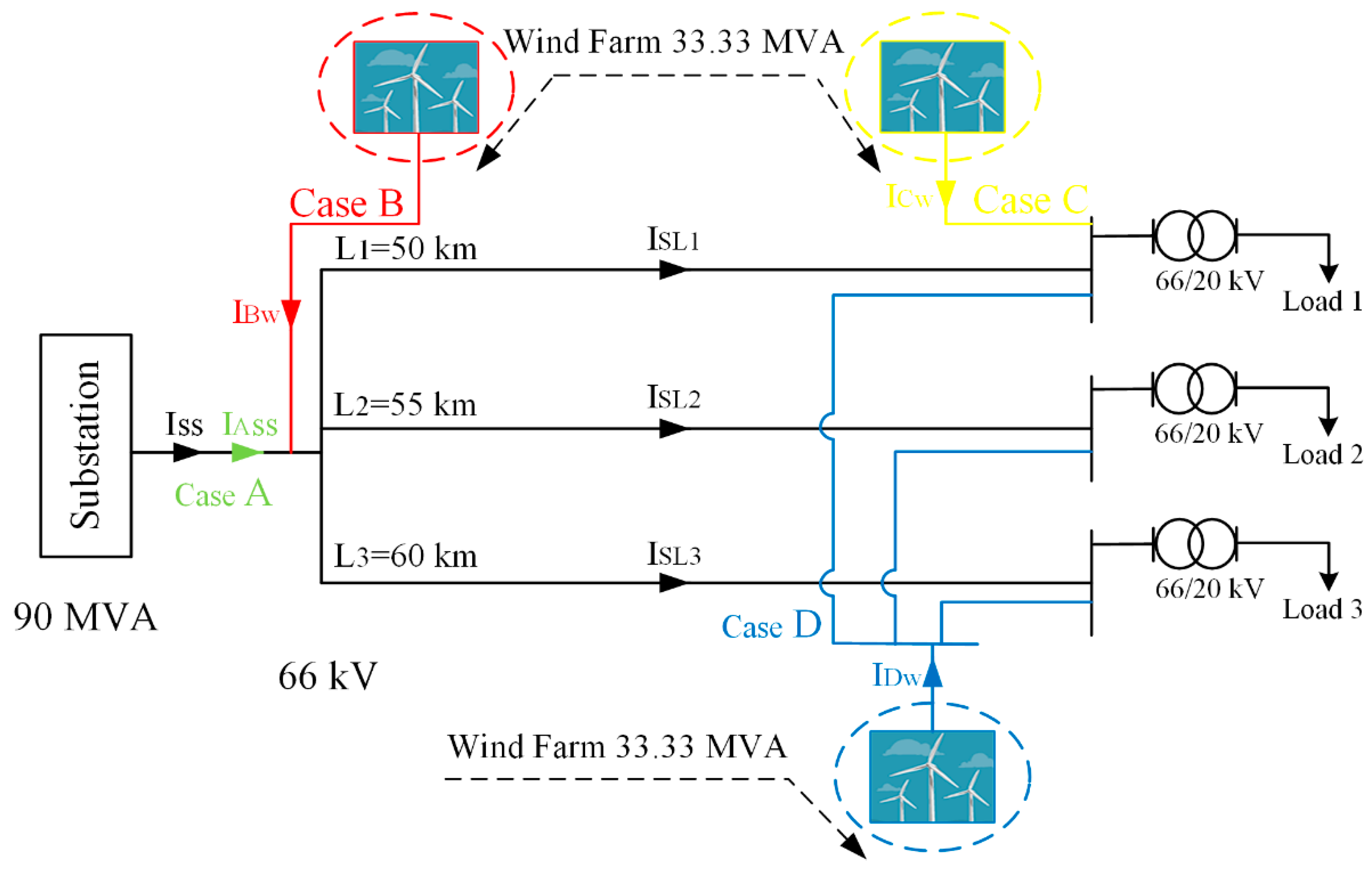
2. System Description

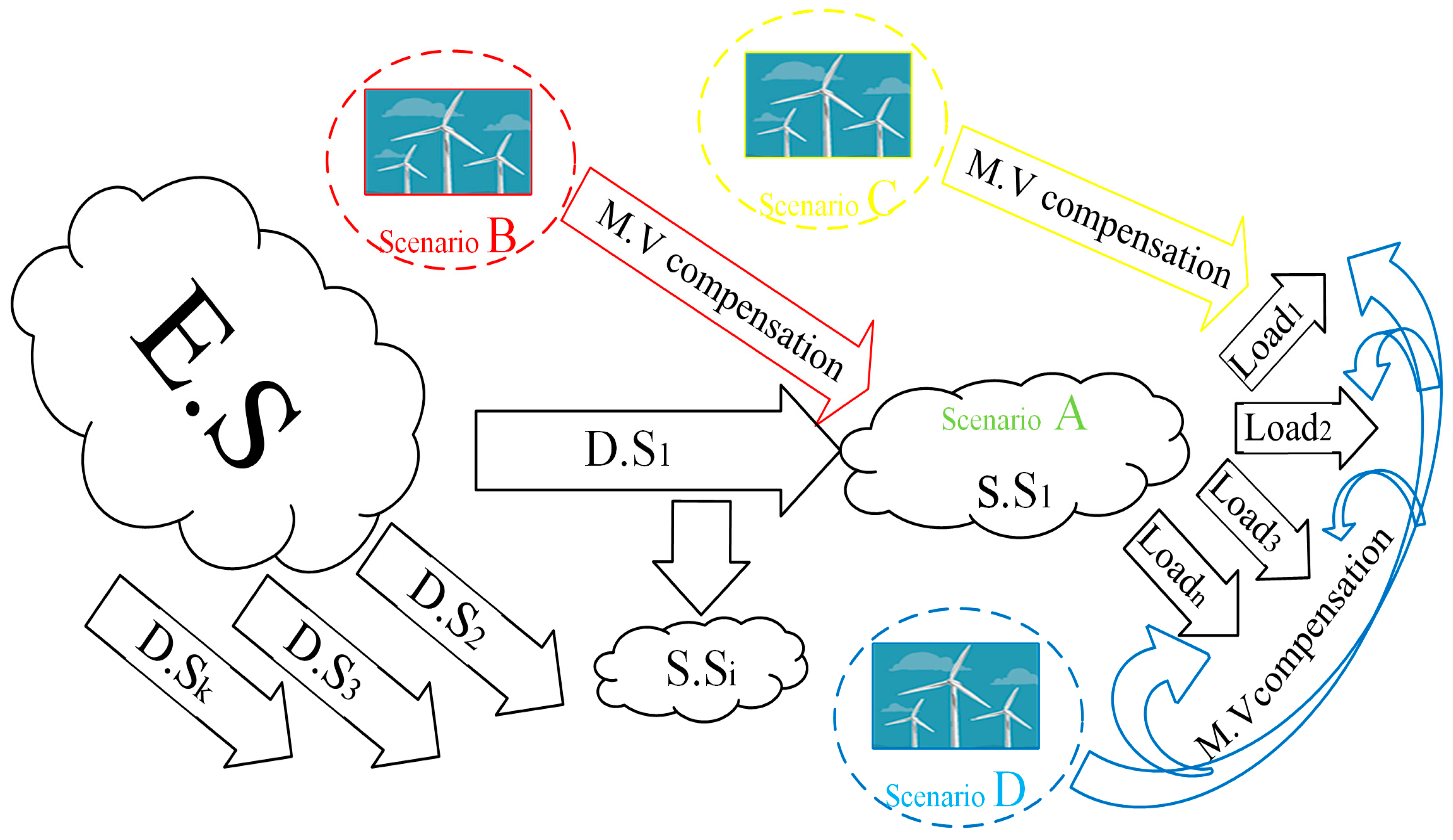
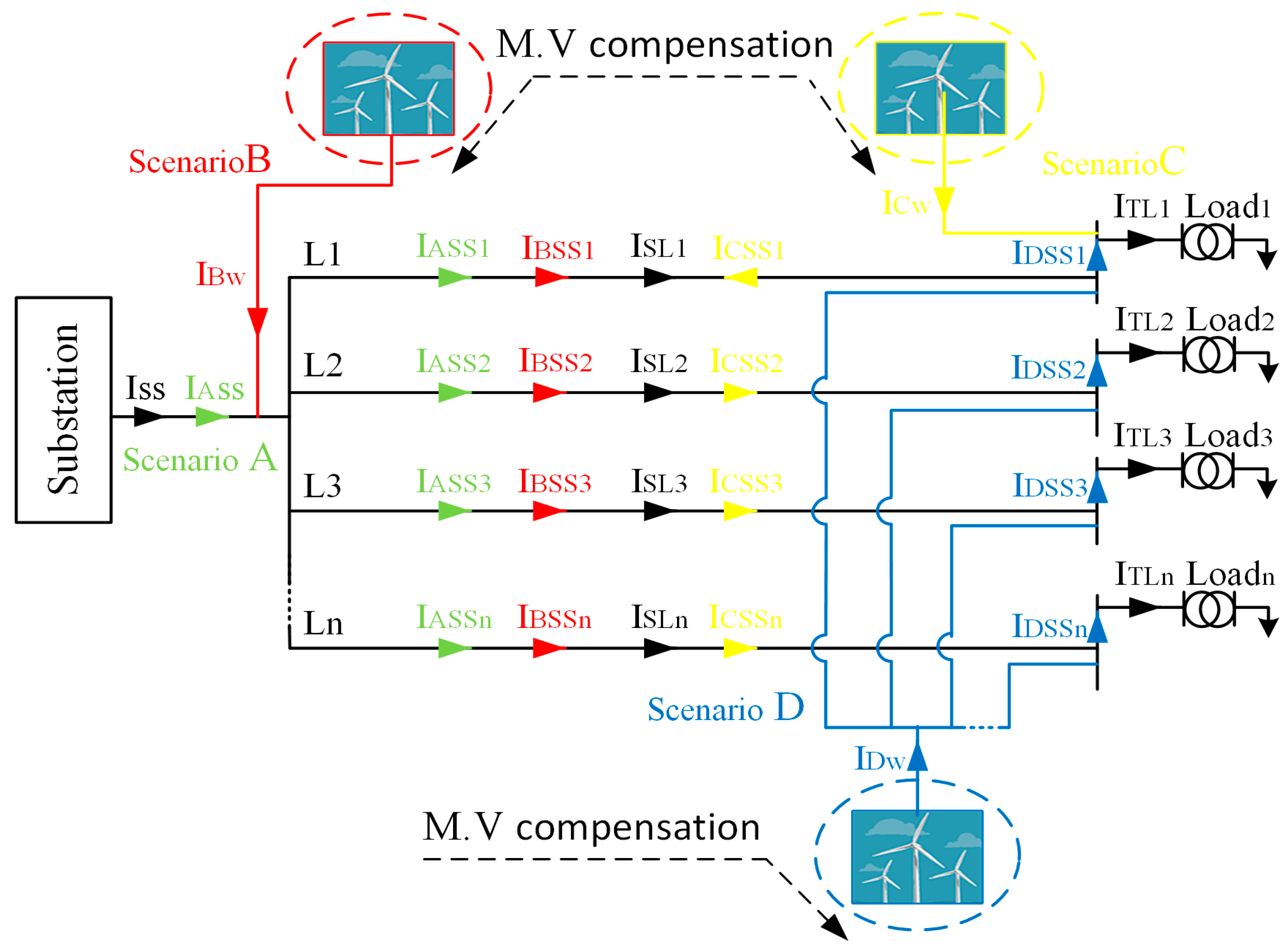
2.1. The Electrical Model and Scenarios

The following function will be used: $f\left(\Delta V,\Delta P\right):A_{ka},L_{kl},D_{kd}$ where we will find the relationship between these parameters and $\left(\Delta V,\Delta P\right)$, so we will change the position of the DG unit and we will use different line lengths and different loads. We can describe the electrical model as follows:

The general electrical system (E.S) supplies power to k distribution systems (D.S_k) and each distribution system supplies different substation systems (S.S_i). So we consider that we have a distribution system (D.S₁) which is connected to a substation system (S.S₁) which in turn supplies n load. The chosen DG unit is a wind farm and this research concentrates on studying how we can control the units to improve voltage profile and reduce power losses, using only the generated reactive power, because we cannot control the generated active power in wind farms. We will discuss the following scenarios which represent $A_{ka}$:

• Scenario A: The wind farm OFF
• Scenario B: The wind farm is connected to the bus bar which supplies all transmission lines.
• Scenario C: The wind farm is connected to the end of one line.
• Scenario D: The wind farm is connected to the end of each transmission line.

The pictorial and schematic descriptions of the system are illustrated in Figure 1 and Figure 2, respectively.

2.2. Wind Farm Model

The wind farm used consists of a synchronous generator and a full-scale IGBT back-to-back voltage source converter so that it can generate reactive power separately of active power and this allows for easy control of the injected reactive power and voltage in a wide range. The active power is a function of the wind speed. The relationship between reactive power and $Q_{ref}$ (which changes between 0 and 1) is linear, where the generated reactive power is the nominal power after multiplying it by the value of $Q_{ref}$.

2.3. Mathematical Model

Considering a medium voltage MV substation system (S.S₁) and its vector components:

$$S_{SS}={\displaystyle \sum }_{i=1}^n{S}_{SLi}$$

(1)

$$I_{SS}={\displaystyle \sum }_{i=1}^n{I}_{SLi}$$

(2)

Hence, for n lines that supply n loads from the MV substation, the set of transformer and load is equal to total load. Thus, the total apparent power of each line is $S_{SLi}$.

From Figure 2:

$$P_{SLi}=\Delta P_{LLi}+P_{LTi}$$

$$\Delta P_{LLi}=P_{SLi}-P_{LTi}$$

(3)

The power losses of the 3-phase line are given by:

$$\Delta P=3I_L{}^2·R_L$$

(4)

and the voltage drop of each phase is given by:

$$\Delta V=I_L·Z_L$$

(5)

considering scenario A:

From (4), and Figure 2 the power losses of line i for scenario A will be:

$$\Delta P_{ALLi}=3\left(I^2{}_{ASSi}·R_{LLi}\right)$$

(6)

where:

$$I_{SLi}=I_{ASSi}$$

(7)

Similarly, from (5), and (7), and Figure 2:

$$\Delta V_{ALLi}=I_{ASSi}·Z_{LLi}$$

(8)

Considering scenario B:

By applying Kirchhoff’s current law we can find:

$$I_{BSSi}=I_{SLi}+I_{BWi}$$

(9)

Also, from (4) and (9), the power losses will be:

$$\Delta P_{BLLi}=3\left(I^2{}_{BSSi}·R_{LLi}\right)$$

$$\Delta P_{BLLi}=3R_{LLi}\left(I^2{}_{SLi}+I^2{}_{BWi}+2·I_{SLi}·I_{BWi}\right)$$

(10)

Similarly, from (5) and (9), and Figure 2:

$$\Delta V_{BLLi}=I_{BSSi}·Z_{LLi}$$

$$\Delta V_{BLLi}=\left(I_{SLi}+I_{BWi}\right)·Z_{LLi}$$

(11)

Considering scenario C:

By applying Kirchhoff’s current law for the line 1:

$$I_{CSS1}=I_{CW1}=I_{CW}-I_{SL1}$$

(12)

Also, by applying Kirchhoff’s current law for the other lines:

$$I_{CSSi}=I_{SLi}+I_{CWi}$$

(13)

From (12) and (13), the power losses of all lines for scenario C is written as following:

$$\Delta P_{CLL1}=3\left({\left(I_{CW}-I_{SL1}\right)}^2·R_{LL1}\right)$$

$$\Delta P_{CLL1}=3\left(I^2{}_{CSS1}·R_{LL1}\right)$$

(14)

$$\Delta P_{CLLi}=3\left({\left(I_{SLi}+I_{CWi}\right)}^2·R_{LLi}\right)$$

$$\Delta P_{CLLi}=3\left(I^2{}_{CSSi}·R_{LLi}\right)$$

(15)

Similarly, from (5), (12) and (13), and Figure 2:

$$\Delta V_{CLL1}=I_{CSS1}·Z_{LL1}$$

(16)

$$\Delta V_{CLLi}=I_{CSSi}·Z_{LLi}$$

(17)

considering scenario D:

By applying Kirchhoff’s current law:

$$I_{DSSi}=I_{SLi}-I_{DWi}$$

(18)

From (4) and (18) the power losses of line i for scenario D is written as following:

$$\Delta P_{DLLi}=3\left({(I_{SLi}-I_{DWi})}^2·R_{LLi}\right)$$

$$\Delta P_{DLLi}=3\left(I^2{}_{DSSi}·R_{LLi}\right)$$

(19)

Similarly, from (5) and (18), and Figure 2:

$$\Delta V_{DLLi}=I_{DSSi}·Z_{LLi}$$

(20)

3. Control Techniques

The general methodology is that we will control the angle between the voltage and current in the chosen dispersed generation unit to generate the suitable reactive power which will reduce the power losses and improve the voltage profile.

3.1. According to the Changes of Reactive Power Demand

In this technique, the wind farm DG unit is used for compensation according to the increase in reactive power demand by utilizing measured reactive power values. Increasing the reactive power of loads must coincide with the increasing of the $Q_{ref}$ which will increase the generated reactive power of the wind farm. The value of $Q_{ref}$ can be calculated by converting the increase in reactive power of loads to relative value and using it as feedback for the wind turbine.

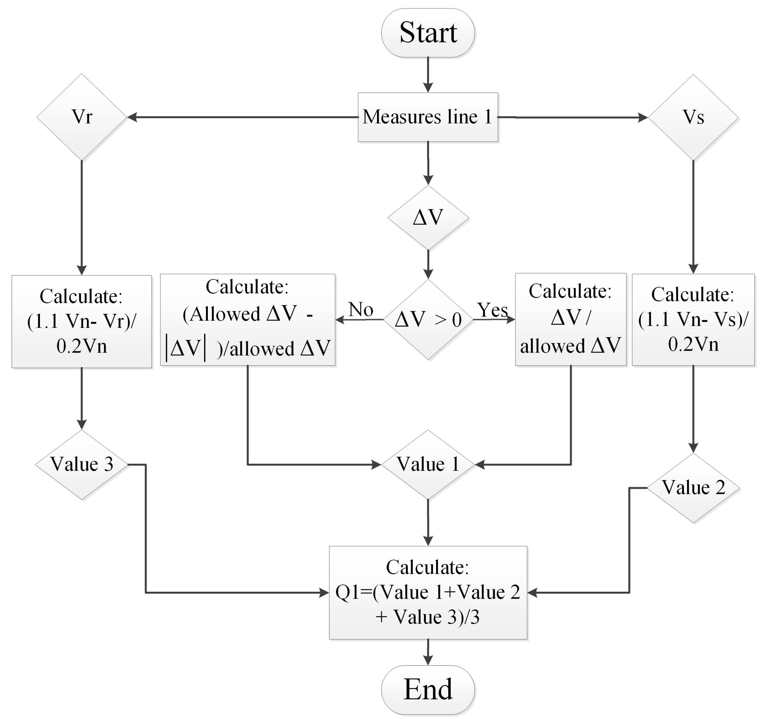
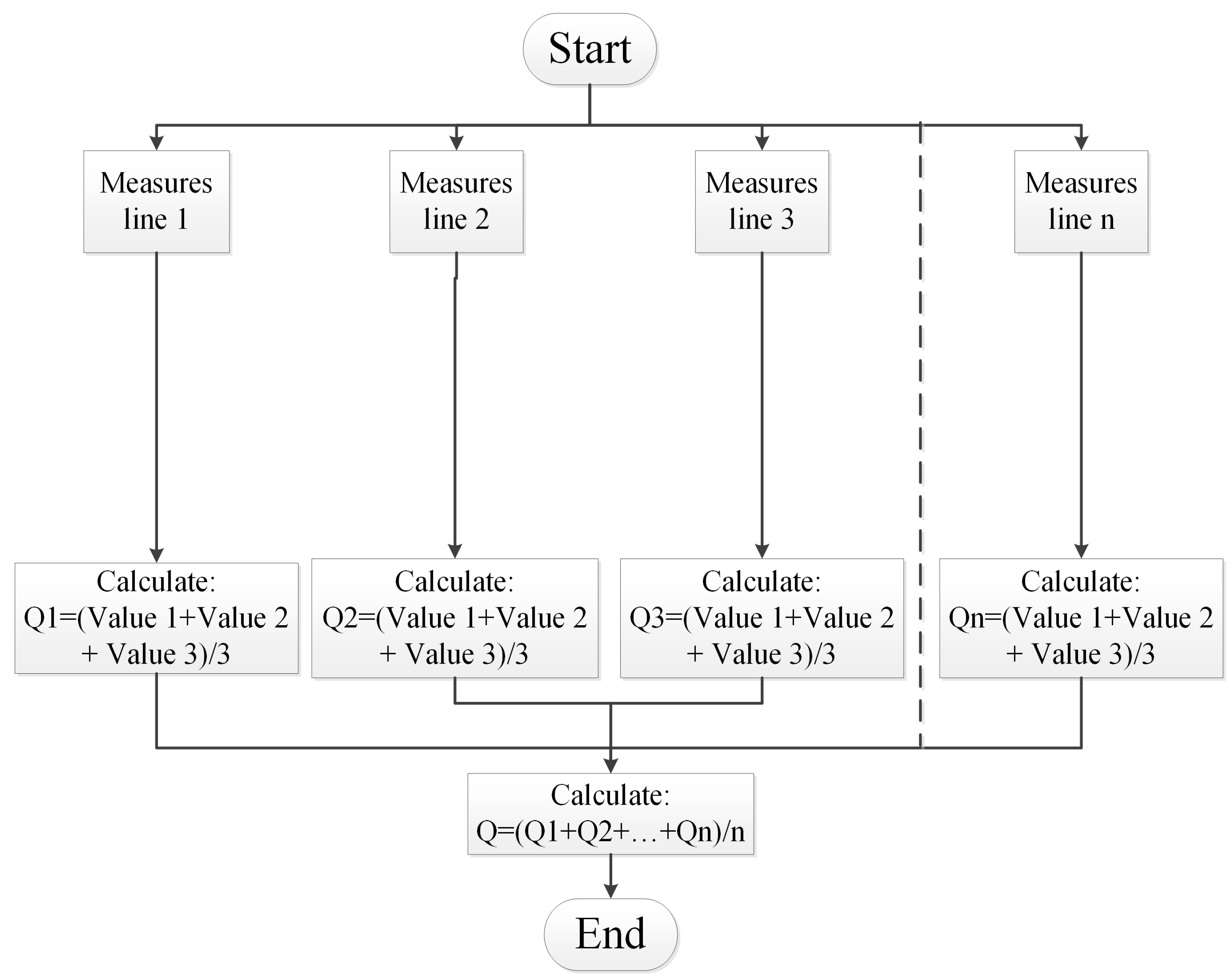
3.2. According to the Changes of Voltage Values

The algorithm used for this method depends on the sending and receiving voltage in addition to the voltage drop for the transmission lines. To apply the algorithm, the following equation below is used for all scenarios:

1. Voltage drop:

Positive voltage drop: implying that the sending voltage is higher than the receiving voltage. The maximum allowable drop in voltage for MV transmission lines is limited to 10% of the sending end bus voltage. Therefore:

$$\mathrm{If}\Delta V_{allowed}\ge \Delta V\ge 0\Rightarrow$$

$$1\ge \frac{\Delta V}{\Delta V_{allowed}}\ge 0\Rightarrow$$

$$1\ge Valu{e}_{i1}\ge 0$$

(21)

$$\mathrm{Else}\Delta V>\Delta V_{allowed}\Rightarrow$$

$$Valu{e}_{i1}>1$$

(22)

When $Valu{e}_{i1}>1$, it implies that voltage drop exceeds the limits, so this value will increase the total value by increasing the generated reactive power.

Negative voltage drop: implying that the sending voltage is lower than the receiving voltage.

Hence:

$$\mathrm{If}\Delta V_{allowed}\ge \left|\Delta V\right|\ge 0\Rightarrow$$

$$0\ge \left|\Delta V\right|-\Delta V_{allowed}\ge -\Delta V_{allowed}\Rightarrow$$

$$0\le \frac{\Delta V_{allowed}-\left|\Delta V\right|}{\Delta V_{allowed}}\le 1$$

$$1\ge Valu{e}_{i1}\ge 0$$

(23)

$$\mathrm{Else}\left|\Delta V\right|>\Delta V_{allowed}\Rightarrow$$

$$Valu{e}_{i1}<0$$

(24)

When $Valu{e}_{i1}<0$ it insinuates that, the voltage drop has exceeded its limits, but in reserve position (that is receiving voltage is higher than sending voltage). These values which are got decrease the total value measured, which further has a decreasing effect on the generated reactive power.

2. Sending voltage:

The changes in sending voltage should not exceed $\pm 10\%$, therefore:

$$\mathrm{If}0.9V_{system}\le V_{Sm}\le 1.1V_{system}\Rightarrow$$

$$-0.9V_{system}\ge -V_{Sm}\ge -1.1V_{system}\Rightarrow$$

$$0.2V_{system}\ge 1.1V_{system}-V_{Sm}\ge 0\Rightarrow$$

$$1\ge \frac{1.1V_{system}-V_{Sm}}{0.2V_{system}}\ge 0\Rightarrow$$

$$1\ge Valu{e}_{i2}\ge 0$$

(25)

$$\mathrm{Else}\mathrm{if}{V}_{Sm}>1.1V_{system}\Rightarrow$$

$$Valu{e}_{i2}<0$$

(26)

When $Valu{e}_{i2}<0$ implying that the sending voltage is very high and exceeds the accepted limits, this observed voltage value will cause a decrease in the total value, thereby bringing about a decrease in the generated reactive power.

$$\mathrm{Else}{V}_{Sm}<0.9V_{system}\Rightarrow$$

$$Valu{e}_{i2}>1$$

(27)

When $Valu{e}_{i2}>1$ indicating that the sending voltage is very low, this voltage value level will cause an increase in the total value, which results in an increase in the generated reactive power.

3. Receiving voltage:

The changes in receiving voltages should not exceed $\pm 10\%$, therefore:

$$\mathrm{If}0.9V_{system}\le V_{Rm}\le 1.1V_{system}\Rightarrow$$

$$-0.9V_{system}\ge -V_{Rm}\ge -1.1V_{system}\Rightarrow$$

$$0.2V_{system}\ge 1.1V_{system}-V_{Rm}\ge 0\Rightarrow$$

$$1\ge \frac{1.1V_{system}-V_{Rm}}{0.2V_{system}}\ge 0\Rightarrow$$

$$1\ge Valu{e}_{i3}\ge 0$$

(28)

$$\mathrm{Else}\mathrm{if}{V}_{Rm}>1.1V_{system}\Rightarrow$$

$$Valu{e}_{i3}<0$$

(29)

When $Valu{e}_{i3}<0$ suggesting that the receiving voltage is very high and exceeds the expected limits, this voltage value level which is got will lead to a decrease in the total value of voltage recorded, and results in a decrease in the generated reactive power.

$$\mathrm{Else}{V}_{Rm}<0.9V_{system}\Rightarrow$$

$$Valu{e}_{i3}>1$$

(30)

When $Valu{e}_{i3}>1$ it conveys the impression the impression that the receiving voltage is very low, this obtained voltage value will give rise to an increase in the total value of voltage. Thereby increasing the value of the generated reactive power.

4. Output value of the algorithm:

This value is $Q_{ref}$ which will cause the generation of suitable reactive power compensation for the MV substation system.

Therefore: the output value of reactive power for each line is:

$$Q_i=\frac{\left(Valu{e}_{i1}+Valu{e}_{i2}+Valu{e}_{i3}\right)}{3}$$

(31)

and the total value for all lines will be:

$$Q_{ref}=\frac{Q_1+Q_2+\dots +Q_n}{n}$$

(32)

The algorithm shown in Figure 3 for 1 line and the algorithm for n lines is presented in Figure 4.

4. Case Study

This section discusses a typical scheme of the commercial electric power system. This is chosen as a benchmark system against which to generate a simulation scheme of the commercial electric power system. The network consists of a 90 MVA sub-transmission station connected with three 66 kV power lines, each line supplies load via a 66/20 kV transformer. The length of each of the MV power lines, $L_1,L_2$ and $L_3$ are 50, 55 and 60 km, respectively. The benchmark electrical network is shown in Figure 5.

Measurements of sending and receiving power (i.e., power losses) and voltage (i.e., voltage drops) for line 1, 2 and 3, were taken in the normal case, this is shown in

Table 1. Measured parameters of the benchmark commercial lines.

Line	${\mathit{P}}_{\mathit{s}}$(MW)	${\mathit{P}}_{\mathit{r}}$(MW)	${\mathit{Q}}_{\mathit{s}}$(MVAR)	${\mathit{Q}}_{\mathit{r}}$(MVAR)	${\mathit{V}}_{\mathit{s}}$(kV)	${\mathit{V}}_{\mathit{r}}$(kV)	$\Delta \mathit{P}$(MW)
1	16.89	16.45	7.11	6.41	64.67	61.38	0.44
2	16.78	16.26	7.08	6.33	64.67	61.09	0.52
3	16.66	16.09	7.02	6.27	64.67	60.87	0.57

. The wind farm rated at 30 MW, 30/0.9 = 33.33 MVA. In creating cases A, B, C and D from scenarios A, B, C and D, respectively, the reactive loads were increased from step 1 to step 5 as presented in

Table 2. Percentage of reactive and apparent power changes for both methods and $Q_{ref}$ values for the first method.

Step	${\mathit{Q}}_{\mathit{L}}\%$	$\mathit{S}$%	${\mathit{Q}}_{\mathit{r}\mathit{e}\mathit{f}}$(p.u.)
1	0%	0%	0
2	33%	3%	0.207
3	66%	7%	0.387
4	100%	12%	0.567
5	133%	17%	0.747

. $Q_{ref}$ values for each step of the first method are shown in Table 2, but for the second method, it changes according to different factors. For cases B, C, and D the reactive power is produced according to $Q_{ref}$. Note that before using the algorithm (that is for the second method), the various cases were designated as cases B, C and D. But after using the algorithm, it is then designated as cases B Reg., C Reg. and D Reg. respectively.

5. Results

In this research, a comparative analysis was used for comparing the results of the two methods and for all the cases. Comparison of one line was done in order to specify the differences easily and clearly. The chosen line is line 2 since it is a normal line and line 3 could have been chosen too whereas we cannot choose line 1, since in case C line 2 is different from all other lines. Therefore, comparing the following five parameters, which are (sending voltage deviation $V_s$%, receiving voltage deviation $V_r$%, voltage drop $\Delta V\%$, power losses $\Delta P\%$ and power factor) will help us to estimate the regulation process. MATLAB Simulink (MathWorks, Natick, MA, USA) was used in the results analyzes.

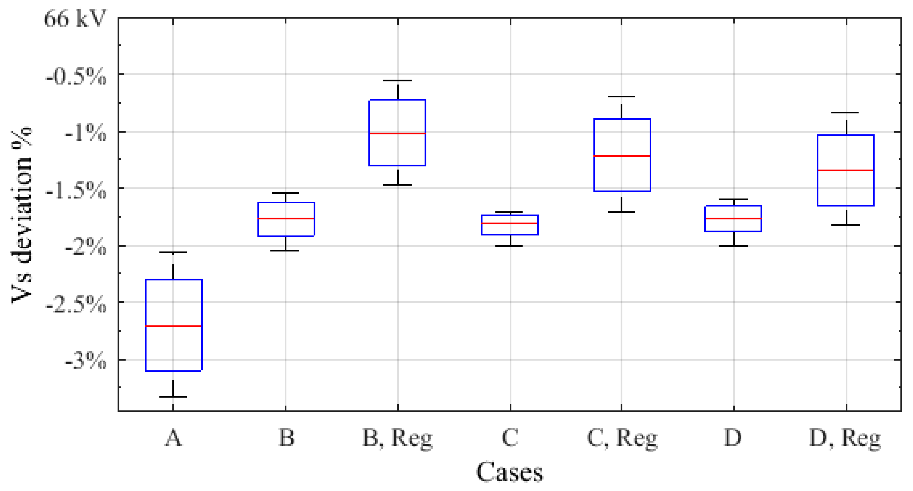
5.1. Sending Voltage Deviation $V_s$%

Figure 6 is a graphical illustration of the sending voltage deviation as a percentage of the nominal voltage of the S.S₁ (66 kV) for all cases where case A is the worst case. It is obvious that connecting the wind farm causes a decrease in voltage deviation for both methods but the second method is better because it takes into account many parameters related to voltage values.

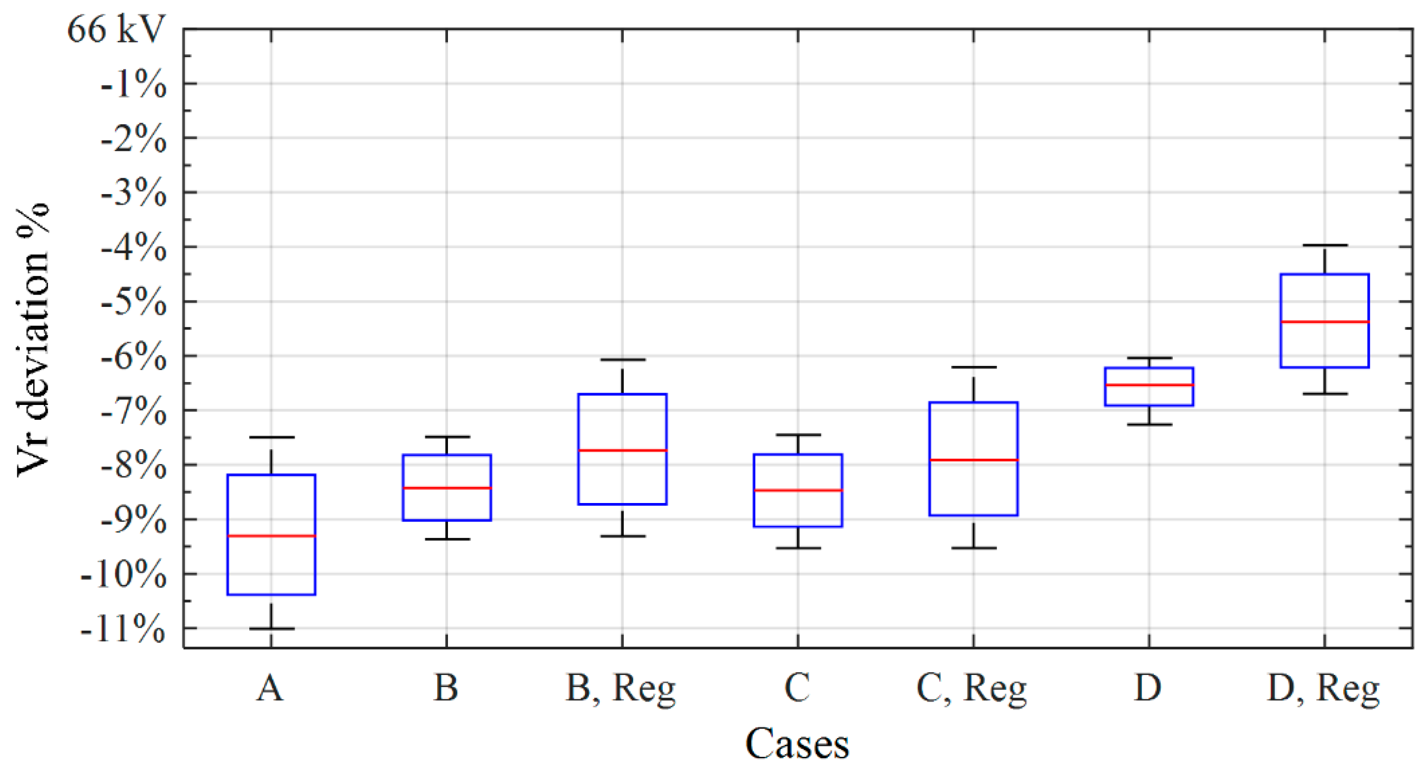
5.2. Receiving Voltage Deviation $V_r$%

Figure 7 illustrates the receiving voltage deviation as a percentage of the nominal voltage of S.S₁ (66 kV) for all cases where case A is the worst case. In a similar way to sending voltage deviation we can find that connecting the wind farm improves the performance of both methods but the second method is better. Also, we can find that case (D) and (D, Reg) are the best-cases where the wind farm acts as a compensator which means that its performance will be better when it is closer to the loads where the current which flows through transmission lines decreases.

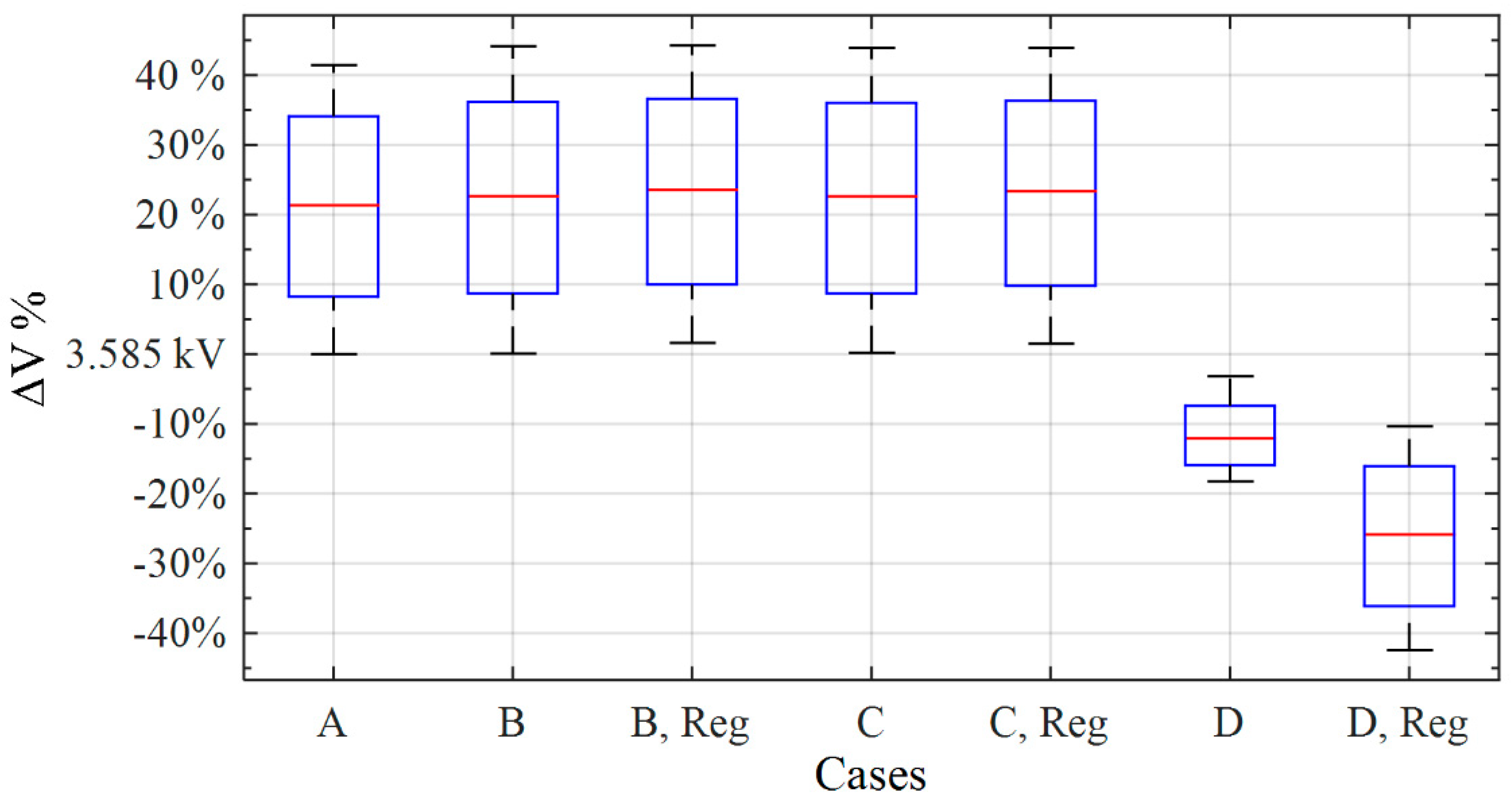
5.3. Voltage Drop $\Delta V$%

Figure 8 illustrates the voltage drop as a percentage of the voltage drop of step 1 of case A (3.585 kV) for all cases where cases (A), (B), (B, Reg), (C) and (C, Reg) are very similar to each other. Cases (D) and (D, Reg) are the best-case scenarios, but case (D, Reg) is better than case (D) so we can conclude that the DG unit can play a role in minimizing voltage drop only if it is close to the loads.

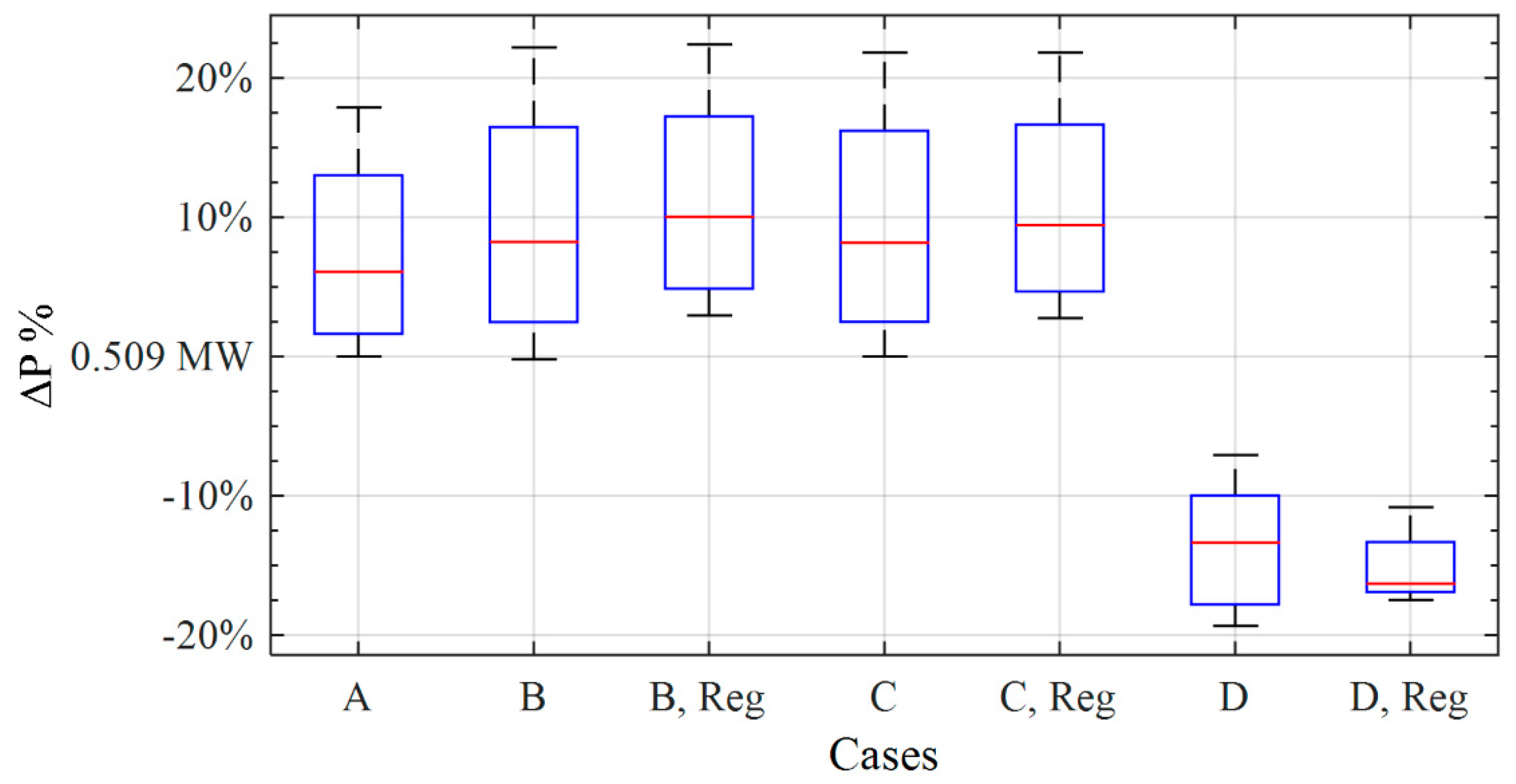
5.4. Power Losses $\Delta P$%

Figure 9, represents the power losses of line 2 as a percentage of the power losses of step 1 of case A (0.509 MW) for all cases wherein a similar way as for voltage drop we can notice that cases (A), (B), (B, Reg), (C) and (C, Reg) have close values of power losses when monitored. Also, we can find that the DG unit as a compensator can reduce power losses only if it is close to the loads.

5.5. Power Factor

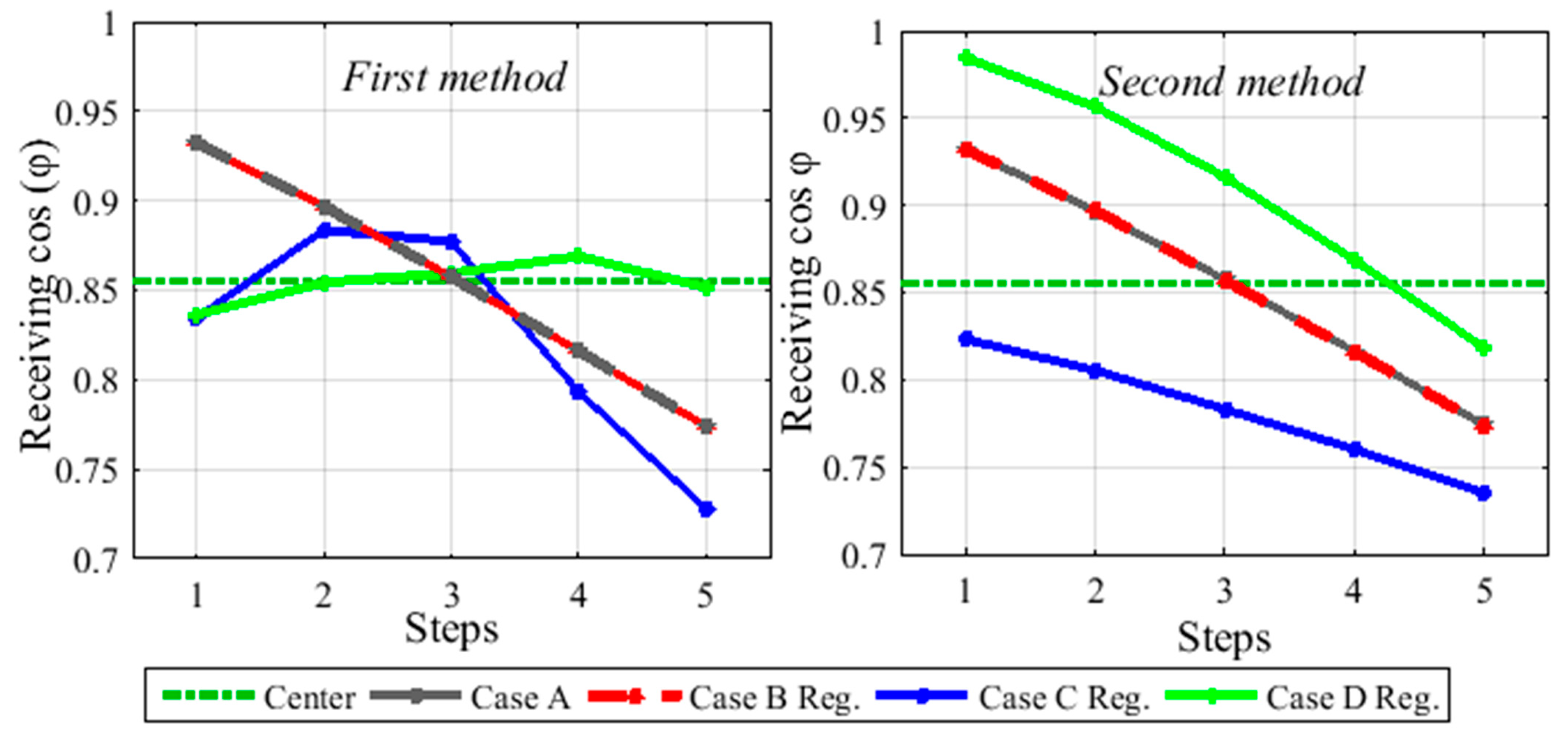
• For the first method: A fast decrease of receiving power factor for Case A and B is observed as shown in Figure 10. It can equally be seen from the figure that the power factor observed in case C is much worse than that of case A and B. The best situation observed is that of case D, the power factor is stable and close values were obtained for all steps monitored.
• For the second method: As shown in Figure 10 it could be observed that case C is the worst situation as compared to other cases. Case A and B have the same values between 0.75 and 0.92. Equally, case D is the best scenario, owing to the fact that the power factor values observed are between 0.84 and 0.99.

5.6. General Comparison

A general comparison is needed to show the general performance of all scenarios before and after using the algorithm. Therefore, Figure 11 shows the general values of all lines and wind speeds for $V_s$, $V_r$, $\Delta V$ and $\Delta P$ parameters for each case as a percentage of Case A. The following observations were made:

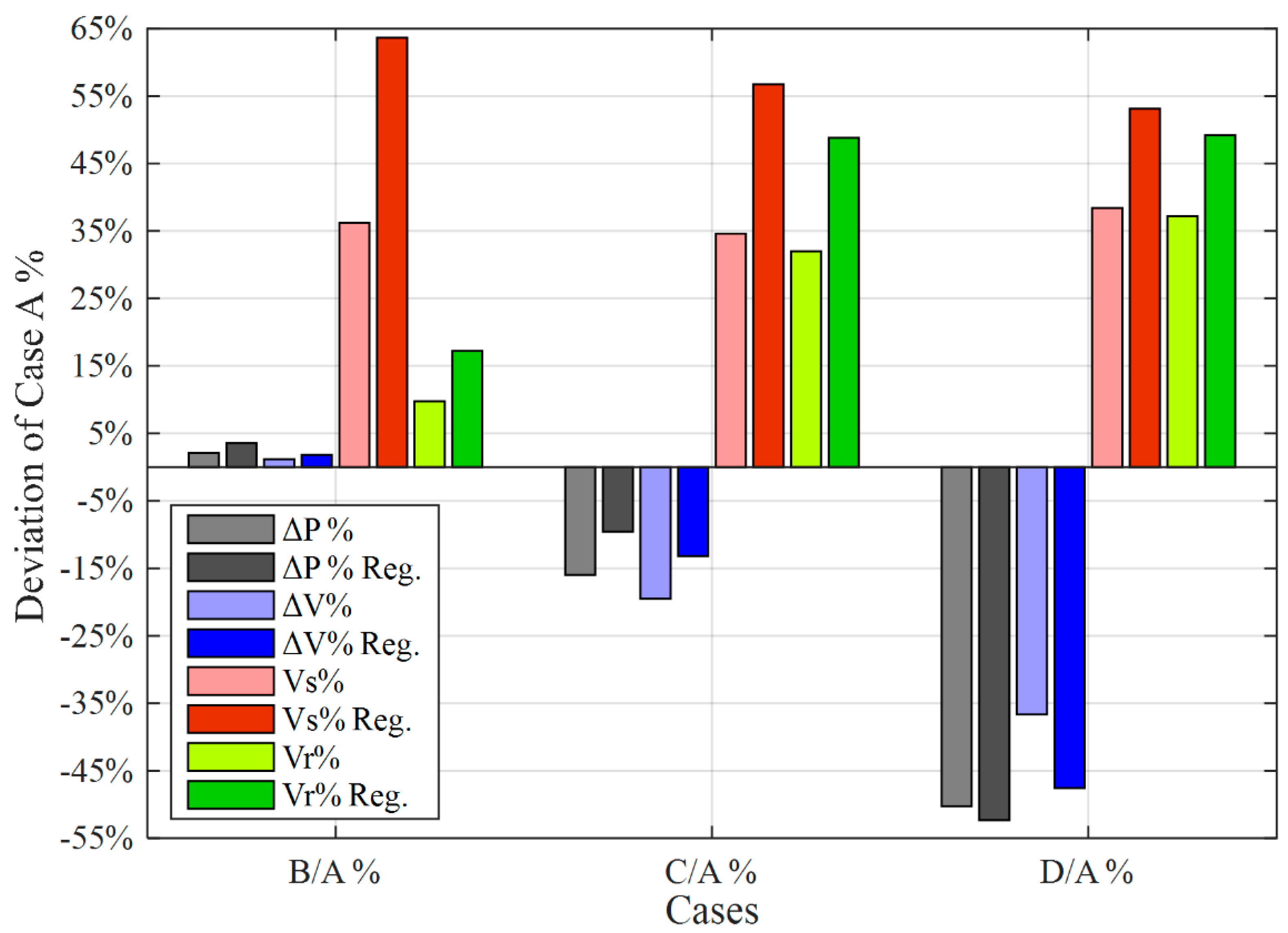
• (Case B/Case A)%: Power losses and voltage drop increased slightly by about 2%, whereas the s% to 64%. Equally, the receiving voltage is observed to increase from 10% to 17%. In general, the performance after using the algorithm is better than before using it.
• (Case C/Case A)%: For power losses and voltage drop a decrease of between (−10% to −16%) for power losses was observed and the voltage drop observed values is between (−14% to −18%), and it is seen that the sending voltage significantly increases from (35% to 56%). Furthermore, ending voltage increased significantly to values between 32% and 48% the receiving voltage increases from (32% to 48%). In general, the performance after using the algorithm is far better than before using it for sending and receiving voltage, but a worse scenario is experienced for power losses and voltage drop.
• (Case D/Case A)%: Power losses decrease from (−50% to −53%) and the voltage drop observed was between (−36% to −47%). The sending voltage increases significantly from (38% to 53%). Additionally, the receiving voltage increases from (37% to 48%). Overall, the performance after using the algorithm is far better than before using it.

According to the results and function $f\left(\Delta V,\Delta P\right):A_{ka},L_{kl},D_{kd}$ the following points can be deduced:

• $A_{ka}$: The position of power injected onto the scheme plays the most vital role in improving voltage profile, minimizing power losses and improving power factor, which according to the results obtained from the scenario for case D is the best scenario for case C is very good and the scenario for case B is good.
• $L_{kl}$: Increasing the loads’ power, especially that of reactive power, results in an increase of voltage drop and power losses and a reduction in the power factor, in which the voltage drop is directly proportional to current and power losses, is the square of the current. Also, the length of the line has an effect on the voltage drop and power losses and power factor. The voltage drop and power losses are directly proportional to the length and resistance of the line, thus increasing the values of loads causes a decrease in the power factor.
• $D_{kd}$: Utilization of the wind farm is dependent on the synchronous generator which generates reactive power and a full-scale IGBT back-to-back voltage source converter, so that it can generate reactive power independently of active power; also, it allows the control and the injection of reactive power and voltage in a wide range of control and in an easy manner. According to the results obtained so far, it is observed that the performance of the S.S1 is better after utilizing the algorithm.

6. Conclusions

DG units can play an important role in improving voltage profiles, reducing power losses and improving power quality in cases of increases in demand for reactive power but the following should be noted:

• The position of the DG unit has a significant role in controlling the voltage and reduction of power losses wherein the DG must be close to the loads which could require additional reactive power.
• The power value of the DG should be closer to the power value of the load because when a DG unit is connected to one line (which supplies smaller load than the DG unit power) the high demand for reactive power will result in problems on the line such as high voltage. Besides, the voltage at the injection point will increase significantly especially when the generated active power is high, such as high wind speed in the case of wind farms or high solar radiation when considering solar farms

Using the proposed algorithm, which takes into account the sending and receiving voltages and voltage drop of all lines, has proved to be very effective, since in some situations of such high reactive power demand DG units could generate high reactive power regardless of the wind speed. In addition, the generated active power is not controlled so it could cause high voltage values for one or more lines but the proposed algorithm can deal with such situations. The algorithm proposed in this paper is totally new and it has been tested in many voltage profile, power loss, and power factor issue scenarios. This algorithm is very effective when a substation is supplied with different generation sources or other renewable energy schemes, such as another wind farm or solar farm, owing to the fact that it takes into account the sending and receiving voltage. The proposed algorithm can be used for different DG units. The recommended future research entails development of the algorithm for transient events (faulted states) in the system.

References

- Liang, H.F.; Yang, L.; You, Y.Y. Research on the Planning of Grid-Connected Capacity of Distributed Generation Based on the Maximum Social Benefits. In Proceedings of the International Conference on Renewable Power Generation (RPG 2015), Beijing, China, 17–18 October 2015; pp. 1–5. [Google Scholar]
- An, A.; Zheng, B.; Zheng, H.; Zheng, C.; Du, P. Benefit Analysis and Evaluation of Distributed Generation in Distribution Network Under Active Management. In Proceedings of the Control and Decision Conference (CCDC), Yinchuan, China, 28–30 May 2016; pp. 6031–6035. [Google Scholar]
- Momoh, J.A.; Xia, Y.; Boswell, G.D. An Approach to Determine Distributed Generation (DG) Benefits in Power Networks. In Proceedings of the 40th NAPS, Calgary, AB, Canada, 28–30 September 2008; pp. 1–7. [Google Scholar]
- Shaw-Williams, D.; Susilawati, C.; Walker, G. Value of residential investment in photovoltaics and batteries in networks: A techno-economic analysis. Energies 2018, 11. [Google Scholar] [CrossRef]
- Grisales-Noreña, L.F.; Montoya, D.G.; Ramos-Paja, C.A. Optimal Sizing and Location of Distributed Generators Based on PBIL and PSO Techniques. Energies 2018, 11, 1018. [Google Scholar] [CrossRef]
- Ghanbari, N.; Mokhtari, H.; Bhattacharya, S. Optimizing Operation Indices Considering Different Types of Distributed Generation in Microgrid Applications. Energies 2018, 11, 894. [Google Scholar] [CrossRef]
- Bhullar, S.; Ghosh, S. Optimal Integration of Multi Distributed Generation Sources in Radial Distribution Networks Using a Hybrid Algorithm. Energies 2018, 11, 628. [Google Scholar] [CrossRef]
- Doğanşahin, K.; Kekezoğlu, B.; Yumurtacı, R.; Erdinç, O.; Catalão, J.P. Maximum Permissible Integration Capacity of Renewable DG Units Based on System Loads. Energies 2018, 11, 255. [Google Scholar] [CrossRef]
- Voropai, N.I.; Efimov, D.N. Operation and Control Problems of Power Systems with Distributed Generation. In Proceedings of the Power and Energy Society General Meeting, Calgary, AB, Canada, 26–30 July 2009; pp. 1–5. [Google Scholar]
- Ali, A.; Boulkaibet, I.; Twala, B.; Marwala, T. Hybrid Optimization Algorithm to the Problem of Distributed Generation Power Losses. In Proceedings of the IEEE International Conference on Systems, Man, and Cybernetics (SMC), Budapest, Hungary, 9–12 October 2016; pp. 001719–001724. [Google Scholar]
- Gkaidatzis, P.A.; Bouhouras, A.S.; Sgouras, K.I.; Doukas, D.I.; Labridis, D.P. Optimal Distributed Generation Placement Problem for Renewable and DG Units: An Innovative Approach; MedPower: Belgrade, Serbia, 2016; pp. 1–7. [Google Scholar]
- Antoniadou-Plytaria, K.E.; Kouveliotis-Lysikatos, I.N.; Georgilakis, P.S.; Hatziargyriou, N.D. Distributed and decentralized voltage control of smart distribution networks: Models, methods, and future research. IEEE Trans. Smart Grid 2017, 8, 2999–3008. [Google Scholar] [CrossRef]
- Villacci, D.; Bontempi, G.; Vaccaro, A. An adaptive local learning-based methodology for voltage regulation in distribution networks with dispersed generation. IEEE Trans. Power Syst. 2006, 21, 1131–1140. [Google Scholar] [CrossRef]
- Brenna, M.; De Berardinis, E.; Carpini, L.D.; Foiadelli, F.; Paulon, P.; Petroni, P.; Sapienza, G.; Scrosati, G.; Zaninelli, D. Automatic distributed voltage control algorithm in smart grids applications. IEEE Trans. Smart Grid 2013, 4, 877–885. [Google Scholar] [CrossRef]
- Elkhatib, M.E.; El-Shatshat, R.; Salama, M.M. Novel coordinated voltage control for smart distribution networks with DG. IEEE Trans. Smart Grid 2011, 2, 598–605. [Google Scholar] [CrossRef]
- Yu, L.; Czarkowski, D.; De León, F. Optimal distributed voltage regulation for secondary networks with DGs. IEEE Trans. Smart Grid 2012, 3, 959–967. [Google Scholar] [CrossRef]
- Molina-García, A.; Mastromauro, R.A.; García-Sánchez, T.; Pugliese, S.; Liserre, M.; Stasi, S. Reactive power flow control for PV inverters voltage support in LV distribution networks. IEEE Trans. Smart Grid 2017, 8, 447–456. [Google Scholar] [CrossRef]
- Liu, H.J.; Shi, W.; Zhu, H. Distributed Voltage Control in Distribution Networks: Online and Robust Implementations. IEEE Trans. Smart Grid 2017. [Google Scholar] [CrossRef]
- Carvalho, P.M.; Correia, P.F.; Ferreira, L.A. Distributed reactive power generation control for voltage rise mitigation in distribution networks. IEEE Trans. Power Syst. 2008, 23, 766–772. [Google Scholar] [CrossRef]
- Saraiva, F.; Nordström, L.; Asada, E. Multi-Agent Systems Applied to Power Loss Minimization in Distribution-Level Smart Grid with Dynamic Load Variation. In Proceedings of the IEEE Congress on Evolutionary Computation (CEC), San Sebastián, Spain, 5–8 June 2017; pp. 217–224. [Google Scholar]
- Tahboub, A.M.; Pandi, V.R.; Zeineldin, H.H. Distribution system reconfiguration for annual energy loss reduction considering variable distributed generation profiles. IEEE Trans. Power Deliv. 2015, 30, 1677–1685. [Google Scholar] [CrossRef]
- Martí, P.; Velasco, M.; Torres-Martínez, J.; Miret, J.; Castilla, M. Reactive Power Control for Loss Minimization in Low-Voltage Distributed Generation Systems. In Proceedings of the International Conference on Control & Automation, Kathmandu, Nepal, 1–3 June 2016; pp. 371–376. [Google Scholar]
- Davda, A.T.; Azzopardi, B.; Parekh, B.R.; Desai, M.D. Dispersed Generation Enable Loss Reduction and Voltage Profile Improvement in Distribution Network—Case Study, Gujarat, India. IEEE Trans. Power Syst. 2014, 29, 1242–1249. [Google Scholar] [CrossRef]
- Georgilakis, P.S.; Hatziargyriou, N.D. Optimal distributed generation placement in power distribution networks: models, methods, and future research. IEEE Trans. Power Syst. 2013, 28, 3420–3428. [Google Scholar] [CrossRef]
- Kumar, P.K. Selection of optimal location and size of multiple distributed generations by using kalman filter algorithm. Int. J. Eng. Res. Appl. 2013, 4, 1708–1729. [Google Scholar]
- Igbinovia, F.O.; Fandi, G.; Müller, Z.; Švec, J.; Tlustý, J. Optimal Location of the Synchronous Condenser in Electric-Power System Networks. In Proceedings of the 17th International Scientific Conference on Electric Power Engineering (EPE), Prague, Czech Republic, 16–18 May 2016; pp. 1–6. [Google Scholar]
- Fandi, G.; Igbinovia, F.O.; Švec, J.; Müller, Z.; Tlustý, J. Advantageous Positioning of Wind Turbine Generating System in MV Distribution Network. In Proceedings of the 17th International Scientific Conference on Electric Power Engineering (EPE), Prague, Czech Republic, 16–18 May 2016; pp. 1–6. [Google Scholar]
- Fandi, G.; Igbinovia, F.O.; Müller, Z.; Švec, J.; Tlusty, J. Using Renewable MV Wind Energy Resource to Supply Reactive Power in MV Distribution Network. In Proceedings of the 16th International Scientific Conference on Electric Power Engineering (EPE), Kouty nad Desnou, Czech Republic, 20–22 May 2015; pp. 169–173. [Google Scholar]
- Fischer, M.; Mendonca, A.; Godin, P. Voltage Control with Wind Farms: Current Practice with Type 4 WTG in Canada; EPEC: Calgary, AB, Canada, 2014; pp. 165–169. [Google Scholar]
- Fandi, G.; Igbinovia, F.O.; Ahmad, I.; Svec, J.; Muller, Z. Modeling and Simulation of a Gearless Variable Speed Wind Turbine System with PMSG. In Proceedings of the PES PowerAfrica, Accra, Ghana, 27–30 June 2017; pp. 59–64. [Google Scholar]