1. Introduction
The requirements for the efficiency of heat exchangers are increasing with the development of modern technologies thus spurring a considerable interest in enhanced compact heat exchangers [
1]. In single-phase flows, maintaining efficient cooling by means of exchangers with mini-channels requires high liquid flow velocities (turbulent flow). Two-phase flow boiling ensures intensive heat transfer at low flow rates [
2]. The advantage of nucleate boiling is that the value of heat transfer coefficient increases with the increase in heat flux and with an inverse dependence on the mass flux. Parallel to the experimental research, theoretical models for boiling in mini-channels have been developed. A series of experimental correlations for predicting local heat transfer coefficient values can be found in References [
3,
4,
5,
6]. Nevertheless, considering that the results published in the literature vary substantially and that the correlations proposed do not ensure satisfactory results, more research on flow boiling heat transfer in mini-channels is still required.
This study describes two-phase flow boiling experiments with ethanol in a rectangular mini-channel. The preset inlet thermal and flow parameters (fluid pressure and temperature, volumetric flow rate, the heat flux generated by the heater), outlet fluid temperature and pressure, temperature distribution on the heater external surface, and void fraction measurements provided data for numerical computations. The distribution of void fraction in the mini-channel two-phase flow was obtained from high-speed camera images. Thermograms of the external heater surface and the external surface in the adiabatic part of the mini-channel allowed producing temperature profiles along the channel length. The read out and computed parameters were then used to solve inverse heat conduction problems.
Modern research often diverges from experiments in favor of numerical simulations based mainly on commercial software, where experimental results only serve to validate numerical calculations, as in References [
7,
8]. The lack of generally accepted prediction techniques causes researchers to continue looking for effective methods of solving heat transfer problems in flow boiling in mini-channels. In this study, two methods based on the Trefftz functions: (1) the Trefftz method and (2) the hybrid Picard–Trefftz method were used to determine the two-dimensional temperature of three elements of a mini-channel. The Trefftz method, belonging to the class of semi-analytical methods, was originally proposed in 1926 by E. Trefftz [
9] for solving linear partial differential equations. The method has been subsequently expanded by many scientist, e.g., References [
10,
11,
12] with a focus mostly on stationary problems. The theoretical foundations and advancement of the Trefftz method are presented in References [
13,
14]. The Trefftz method has been used in combination with other methods such as the Finite Element Method (FEM) [
15], the homotopy perturbation method [
16], Beck’s method [
17] and the radial basis functions method [
18].
In this paper, Trefftz functions were used to solve a triple coupled inverse heat conduction problem (IHCP) in forced flow boiling in a rectangular asymmetrically heated mini-channel. The experiment aimed to describe low Reynolds number flows (for Re between 17 and 51), thus, it seemed reasonable to assume the laminarity of the flow. All data were taken under stable stationary inlet conditions. After each change of the inlet parameters, such as the volume flow rate, inlet pressure, inlet liquid temperature, and electric current supplied to the heater, new data were taken after a certain period of time necessary to observe stable values of the recorded parameters.
The temperature distributions in the boiling liquid, heating foil, and insulating foil were described with the energy equation, Poisson equation, and Laplace equation, respectively. For all these elements the boundary conditions corresponding to the observed physical process were indicated. Inverse problems in the three adjacent regions with different physical parameters were considered. The Trefftz method was used to obtain the 2D temperature distributions of the two mini-channel elements (the insulating foil and the heater). Two-dimensional fluid temperatures were calculated with the use of the hybrid Picard–Trefftz method. The heat transfer coefficient at the heater-liquid interface was determined based on the Robin boundary condition. Local values of the heat transfer coefficient calculated with Picard–Trefftz method were compared with the values obtained with a simplified 1D approach.
2. Experiment
2.1. Experimental Stand
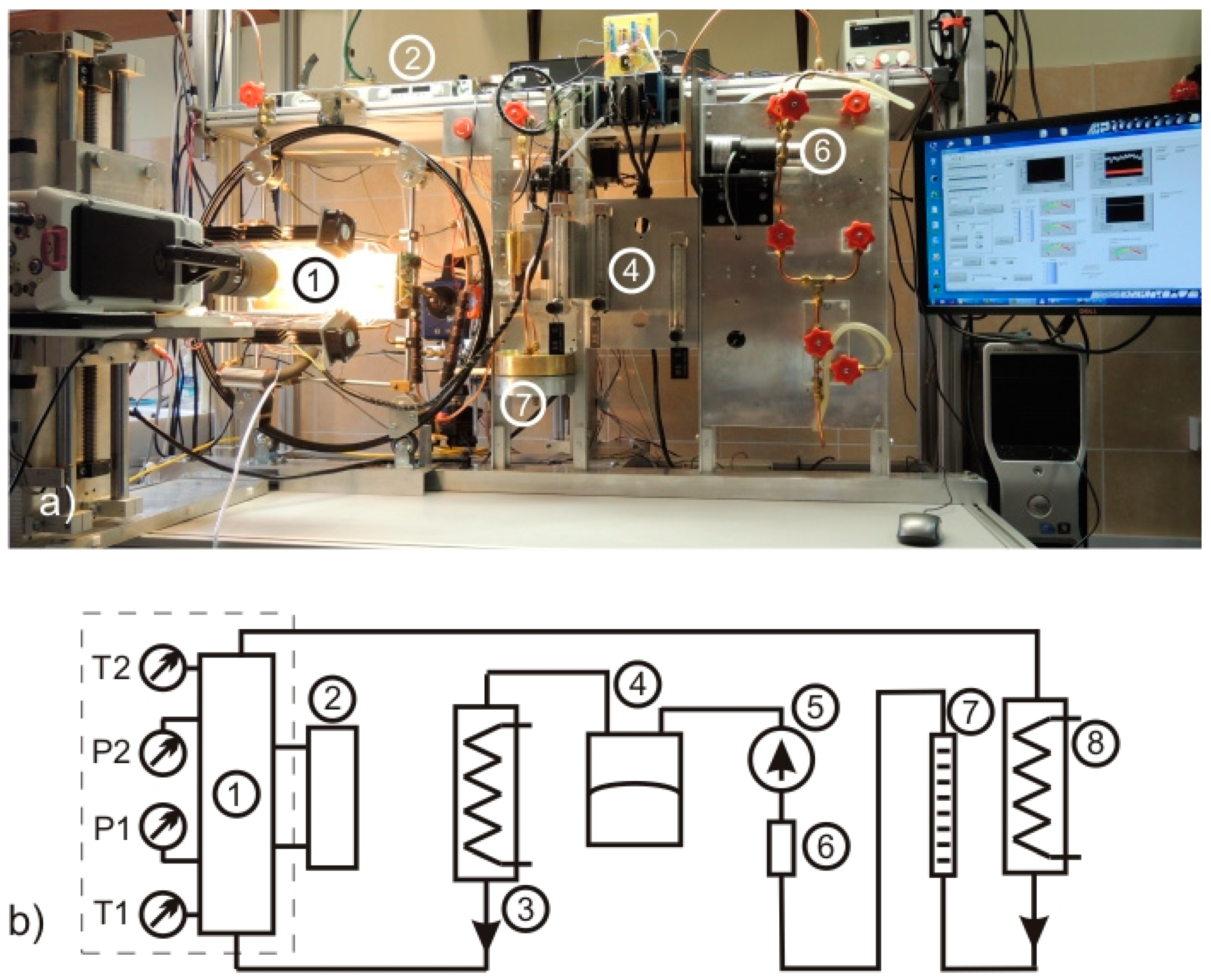
Figure 1 shows both a photo and a schematic view of the experimental setup.
The main element of the system is the test section containing a milled 193 mm long, 1.8 mm deep, and 2 mm wide mini-channel with a hydraulic diameter of 1.89 mm and a cross-sectional area of 3.6 mm
2 (
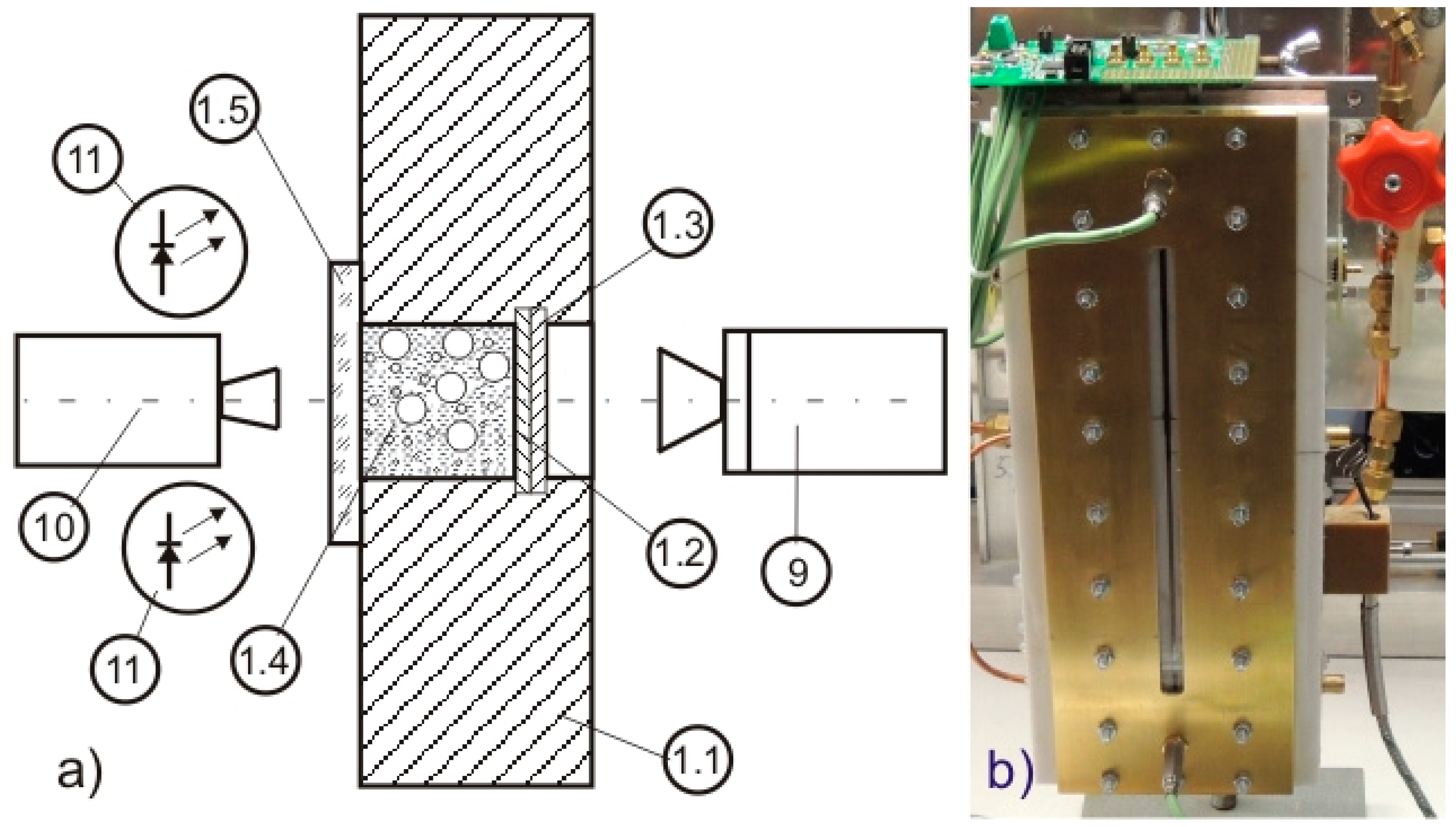
Figure 2). The mini-channel is closed on one side with a transparent sight window for recording flow images with a high-speed camera (Phantom 711, Vision Research Company, Wayne, NJ, USA);
Figure 2. The second wall of the channel is a flat DC powered Kanthal resistance strip heater, 0.1 mm thick and 93 mm long (
Figure 1). The heater is insulated with a 0.18 mm thick 3M Scotch Super 33+ electrical tape, in which the two-dimensional temperature distribution was recorded using the infrared camera (
Figure 2). The test section is also equipped with sensors for pressure and temperature measurements (
Figure 1). The liquid of the preset temperature enters the mini-channel and is heated while flowing through the heater. Upon leaving the mini-channel it is directed to the cooler, then to the rotameter and through a filter to a precision micropump (
Figure 1). The micropump pushes the liquid into a diaphragm pressure generator in which a thin rubber diaphragm separates the compressed air from the liquid (
Figure 1). In order to avoid heating the flowing liquid within the candescent light, customized LED lighting was developed (
Figure 2).
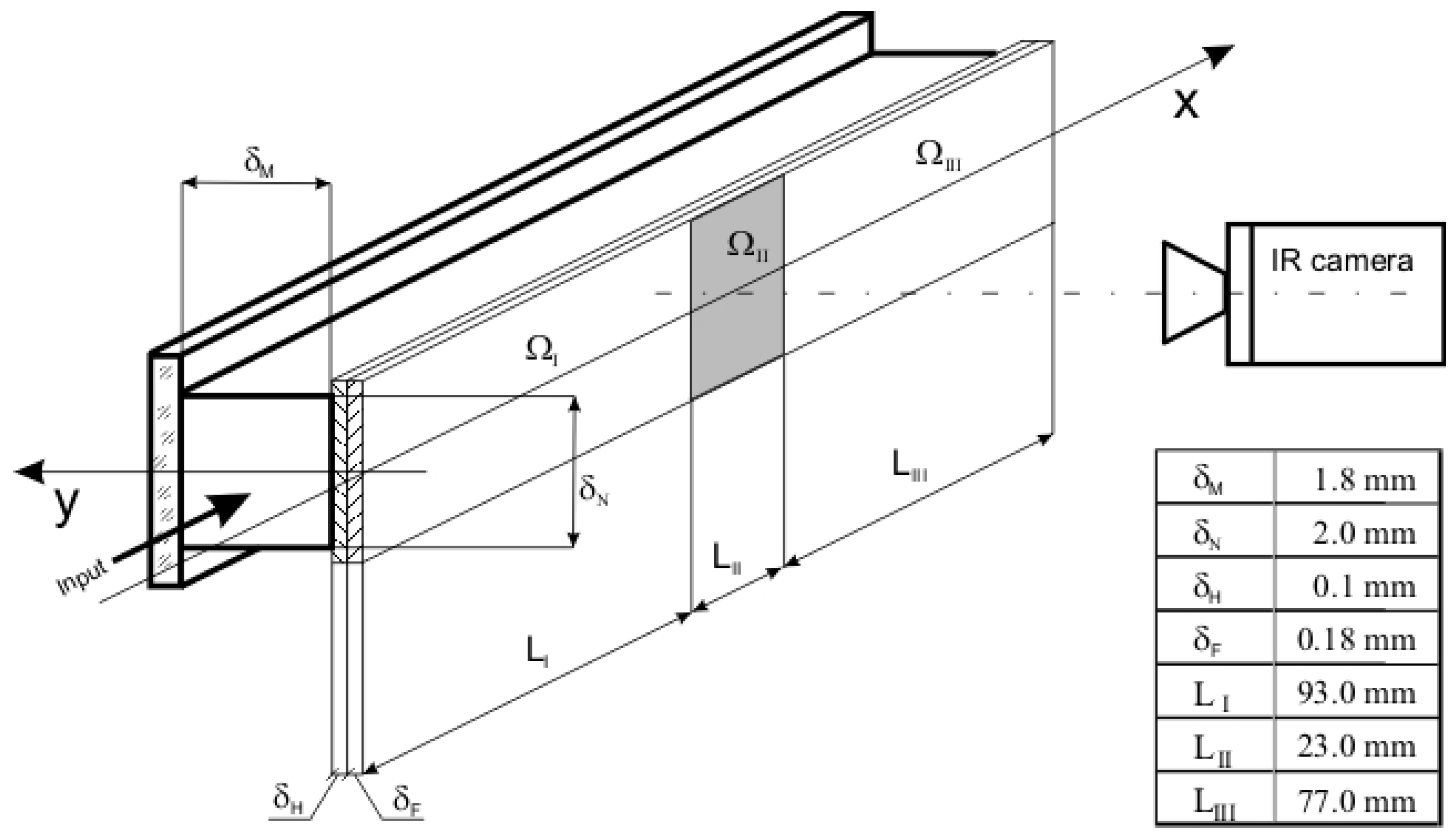
For the purpose of this experiment, the mini-channel was split into three domains corresponding to the heat supply method used (
Figure 3). In the Ω
I domain, the heat supplied to the liquid was generated by the electric heater. Due to design reasons, it was not possible to record the temperature field in the insulating foil of the Ω
II domain. The Ω
III domain was quasi-adiabatic and all thermal and flow parameters were recorded there, just as in Ω
I.
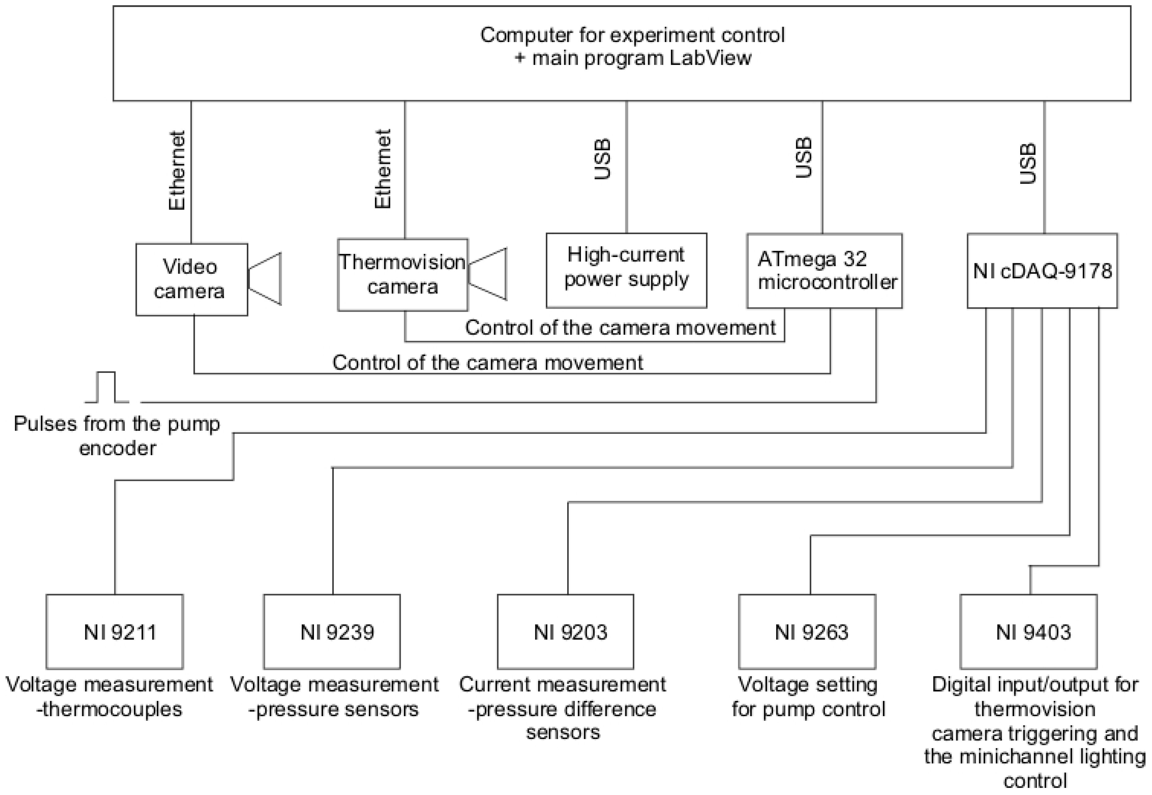
The data were read and recorded using the measurement and control system based on the National Instruments modules (
Figure 4). The main module was the NIcDAQ-9178 (National Instruments Corporation, Austin, TX, USA) in which ancillary modules were installed to measure process parameters and to control components such as a pump, lighting, a camera trigger, etc. The following modules were used:
NI cDAQ-9178: main module,
NI 9211: temperature measurement (Czaki TP-201 type K thermocouples, Czaki Thermo-Product, Pruszków, Poland),
NI 9239: voltage measurement (Kobold pressure gauges, 0–2.5 bar measurement range),
NI 9203: current measurement (Kobold pressure drop gauge, 0–2.5 bar),
NI 9263: adjustment of voltage to control the pumps,
NI 9403: digital input/output to control mini-channel lighting and to trigger the thermal imaging camera.
The main module communicated with the computer for experiment control computer via USB. The experimental stand was controlled by software developed in the LabView environment, chosen due to its versatility and full support of the control and measurement modules. The cameras were shifted using a specially constructed for this purpose module based on the ATmega 32 microprocessor (Atmel Company, San Jose, CA, USA) and controlled by dedicated software developed in the BASCOM environment (MCS Electronics, Almere, The Netherlands).
2.2. Experimental Results
The experimental setup thoroughly described in Reference [
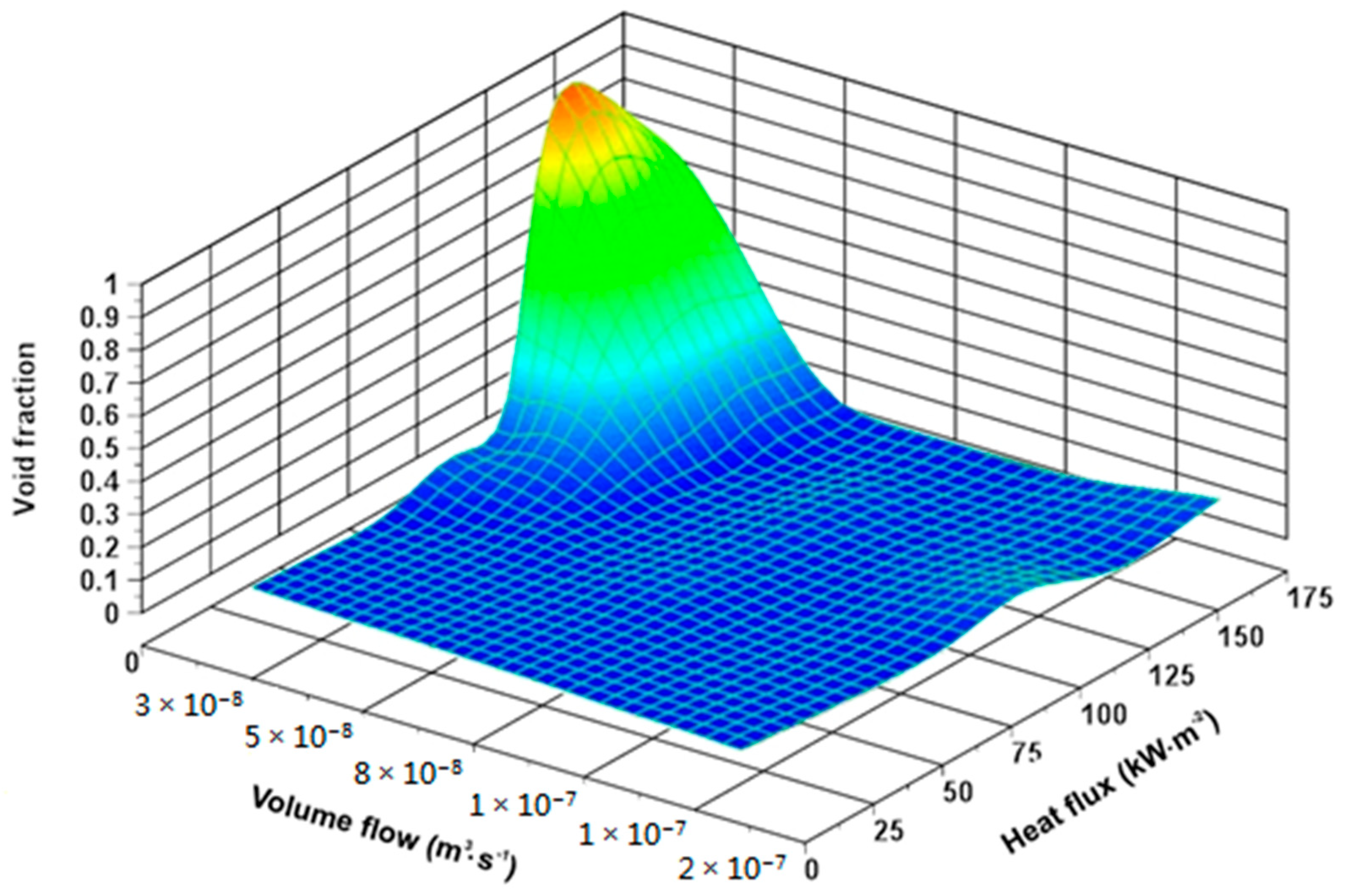
19] was designed to study the flow of the liquid at a set rate and the temperature and pressure at the inlet to the mini-channel; to heat the liquid in the mini-channel to the set temperature; to measure and record the temperature and pressure at the inlet and outlet of the mini-channel, the liquid volumetric flow rate, and the electric current supplied to the heating foil; and to record the flow structures and two-dimensional temperature distributions on the outer surface of the insulation foil. The tests included the determination of the influence of the volumetric flow rate and heat flux changes on the change in the liquid temperature along the mini-channel from the temperature at the outlet to the temperature at the mini-channel inlet. Observations of the two-phase flow structures helped determine the void fraction (
Figure 5). The method of determining the void faction was described in detail in Reference [
20].
This method is based on the script developed in a Matlab 2012 environment (MathWorks, Natick, MA, USA) that uses two toolboxes: Computer System Vision and Image Processing Toolbox 2012 (MathWorks, Natick, MA, USA). The script enables the following operations: image analysis, object segmentation, image enhancement by sharpening and noise reduction, and geometric transformations, as well as object detection and spatial dimensions determination, which subsequently lead to the designation of the void fraction in the mini-channel.
3. Mathematical Model and Methods
The 2D mathematical model included the assumption that the flow was laminar and that the physical parameters of the measurement module were time independent. Their changes in the insulating foil, heating surface, and liquid were assumed to be minor across the mini-channel width [
19].
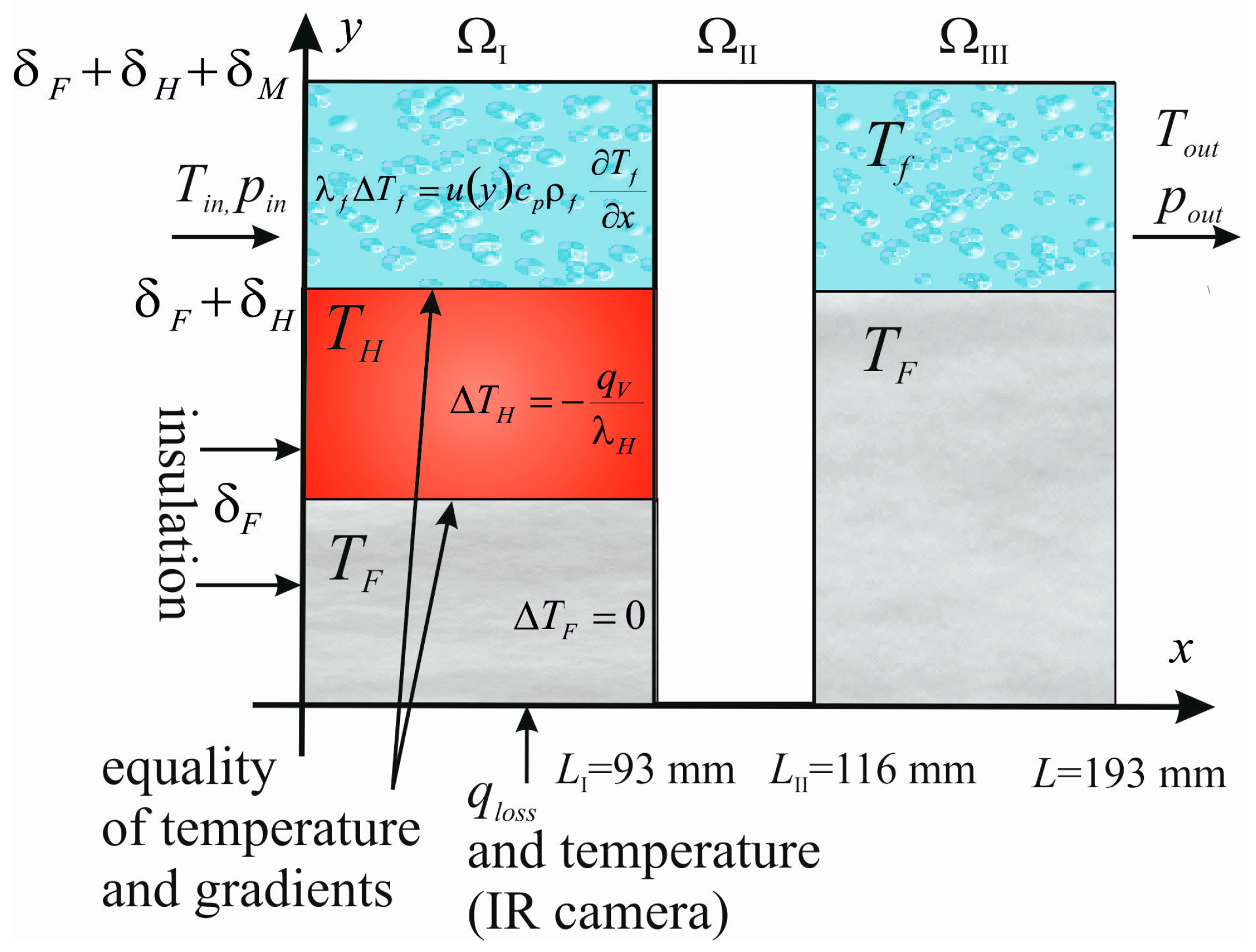
Two dimensions perpendicular to each other were factored in the model: dimension
x in the direction of two-phase flow and dimension
y referring to the foil thickness, to the heater and to the depth of the mini-channel (
Figure 6). Further, in the article, only the central part of the test section along its length will be considered. Due to the design of the test section (
Figure 6), the heat transfer mathematical model was built for the first domain, Ω
I, containing the heater. The temperature of the insulating foil
TF and the temperature of the heater
TH were assumed to satisfy Laplace’s equation and Poisson’s equation, respectively
For Equations (1) and (2), the following boundary conditions were adopted:
where the heat loss
qloss was determined following the procedure given in Reference [
15]. The insulating foil layers and the heater were considered to be in perfect thermal contact, i.e.,
The fluid temperature in the domain
satisfied the energy equation
Adequate boundary conditions were adopted for Equation (9) [
21]:
The heat transfer coefficient at the heater-liquid interface was determined using the boundary condition of the third kind:
The reference temperature
Tave was the average liquid temperature along the mini-channel depth
3.1. Hybrid Picard–Trefftz Method
Two-dimensional approximations of the insulating foil and the heater temperatures were calculated by the Trefftz method by analogy to Reference [
22]. The unknown solutions of Equations (1) and (2) were approximated by a linear combination of the Trefftz functions (the harmonic polynomials in this case). The coefficients of a linear combination were to be determined so that the approximate solutions would satisfy the boundary conditions (Equations (3)–(8)) in the least-squares sense as in References [
15,
19,
21,
22,
23,
24].
Equation (9) was solved with a combination of the Picard and Trefftz method. This equation with the adequate boundary conditions can be written using operator notation
where differential operator
N is defined as
and operator
B describes the boundary conditions that are satisfied by the function
Tf at the boundary
∂Ω
I,f of the domain. Generally, the operator
N can be non-linear and the procedure of determining the solution of Equation (9) can be applied to determining the solutions of non-linear differential equations [
23].
The following procedure, supported by the Picard iterations, was used to approximate the solutions to Equation (15):
In the first step, for
k = 1:
In subsequent steps, for
k > 1:
In each consecutive step, the approximate solutions to Equations (18) and (20) were found using the Trefftz method, expressed in the following form
Function
is a particular solution to the Poisson’s Equation (20), and for Equation (18), the particular solution
. To find the particular solution
, the Taylor series expansion of
is used (expansion about point (0, 0) for simplified representation). Then the particular solution
(for
k = 2, 3, …) is found based on the formula
where, for the monomials in the Taylor series of the function
, operator Δ
−1 is defined by the formula
The coefficients of the linear combinations in Equation (22) were determined based on the adopted boundary conditions, following the method described in References [
22,
24].
3.2. One-Dimensional Approach
In order to verify the results of the hybrid Picard–Trefftz method, the heat transfer coefficient was determined by adopting additional simplifications. It was assumed that Equations (3), (4) and (7) and the heat flux transferred to the fluid by the heater were constant, i.e.,
Individual elements of the test section create a system of planar layers with different thicknesses and thermal conductivity. Since the thickness of the insulating foil and that of the heater are very small, it was possible to replace the partial derivatives in Equations (4) and (25) with a finite difference
Combining Equations (3), (7), (26) and (27) the following formula was obtained for the heater temperature at the boundary
y = δ
F + δ
H:
Then the heat transfer coefficient at the heater-ethanol contact could be determined using the following condition
4. Results and Discussion
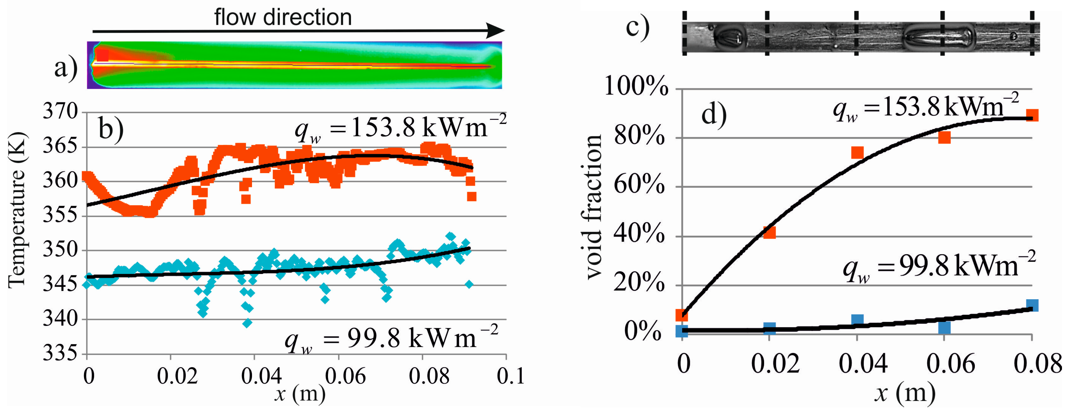
Numerical calculations were performed for the experimental data acquired for ethanol under two-phase flow conditions in the asymmetrically heated mini-channel. Measurements of the insulating foil temperature based on the data from the thermal imaging camera (
Figure 7a) were approximated by a third-degree polynomial (
Figure 7b). The void fraction determined in the manner described in Reference [
20] at distances of 0 mm, 20 mm, 40 mm, 80 mm from the mini-channel inlet was also approximated by a polynomial (
Figure 7c).
Numerical calculations were made for the following experimental data: an inlet pressure 1.1 kPa (average), a liquid temperature at the inlet 308 K (average), a mass flow 21 kg m
−2 s
−1, and six heat flux densities in the range of 99.8–153.8 kW m
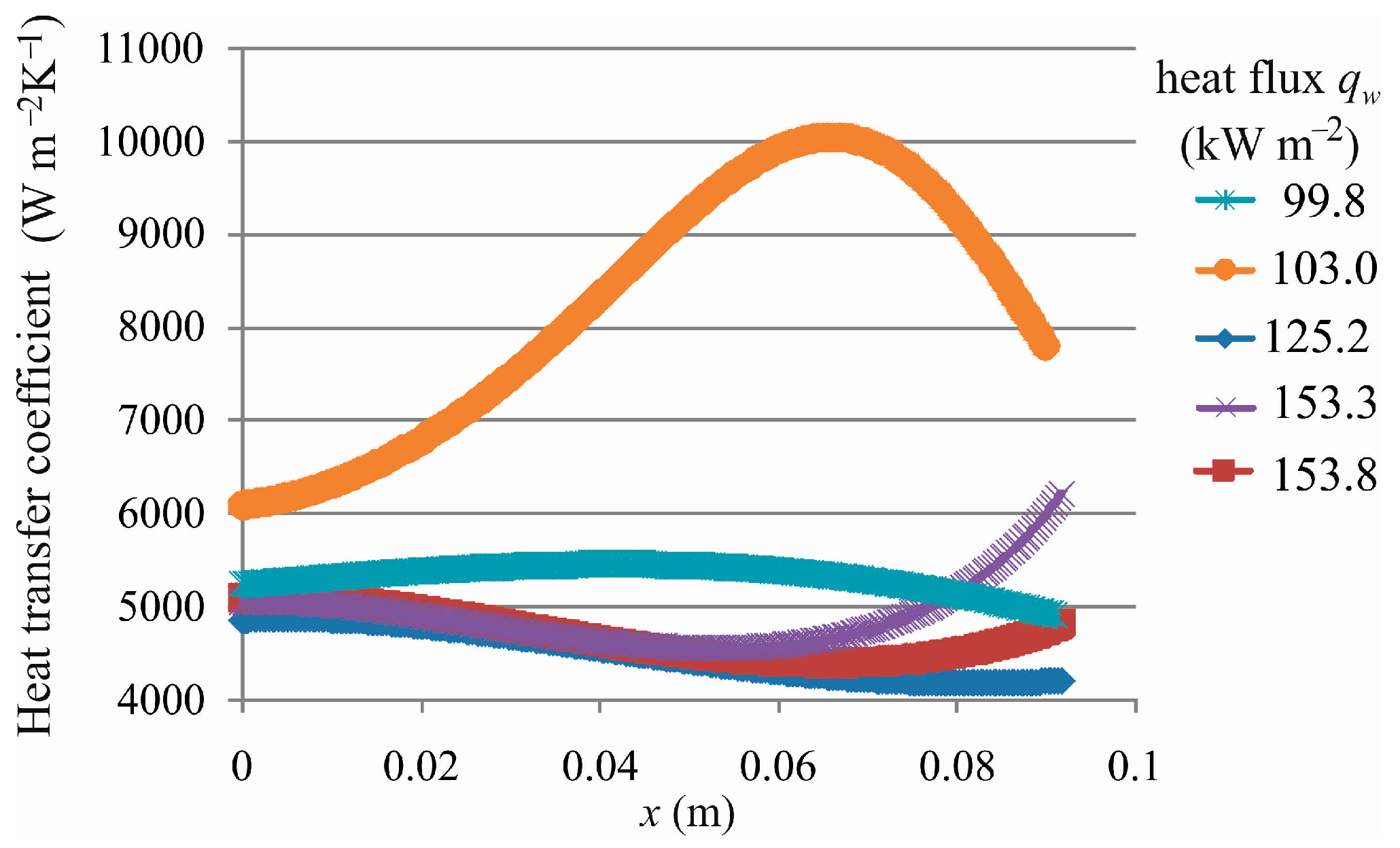
−2. In the first place, 2D temperature distributions in the insulating foil and in the heater were determined using the Trefftz method with six Trefftz functions. In the next stage, the hybrid Picard–Trefftz method was used to determine the 2D liquid temperature distribution with four iterative steps and two harmonic polynomials at each step. The values of the local heat transfer coefficients obtained from Equation (13) based on the hybrid Picard–Trefftz method are shown in
Figure 8. The heat transfer coefficients take values from 4000 Wm
−2 K
−1 to 6000 Wm
−2 K
−1 and, except one case described below, show low variability along the mini-channel length.
The plot of the heat transfer coefficient variation for
qw = 103 kW m
−2 is different from the plots of the other functions as the result of low void fraction values. In this case, it was not more than 7% for
x =
LI, whereas in other cases, it was at least 12% at
x =
LI. A further increase in the heat flux resulted in an increased void fraction and a reduced heat transfer coefficient. The maximum relative differences
(MRD) describing the difference between the heat transfer coefficients, obtained from Equations (13) and (29) were calculated from the formula
where
–norm is, in this case, defined as
For all the heat fluxes considered, the maximum relative differences (
MRD) ranged from 2.4% to 8.7%. The results obtained using the numerical methods were summarized, compared, and found to be similar. The mean relative error of the heat transfer coefficient α
2D was determined from the formula
where, in the calculations, the following were adopted:
The uncertainty of thermal conductivity: ∆λH = 0.1 Wm−1 K−1 (specified by the manufacturer);
The accuracy of the foil temperature approximation:
and
= 10
−4 m [
25], and the uncertainty of temperature measurement is equal to
= 0.55 K (specified by the manufacturer);
The accuracy of the derivative of the approximate foil temperature with respect to y: ;
The accuracy of the reference fluid temperature determination:
For the one-dimensional approach, the mean relative errors ε
1D of the heat transfer coefficient α
1D was calculated by analogy to ε
2D.
Table 1 compares the mean relative errors of the heat transfer coefficients α
2D and α
1D for the considered heat fluxes.
The values of the mean relative errors ε1D are smaller than those for two-dimensional approach ε2D. The mean relative error ε2D does not exceed 4.54% and ε1D oscillates around 2% (maximum 2.36%). The errors decrease with the increasing heat flux supplied to the heater except for the case of qw = 103.0 kW m−2.
5. Conclusions
The application of numerical methods to the identification of temperature distribution and heat transfer coefficient in the flow boiling of ethanol in a horizontal mini-channel was proposed. The use of (1) the Trefftz method and (2) the hybrid Picard–Trefftz method allowed solving three consecutive heat conduction problems in three different elements of the test section: the insulating foil, the heating foil, and the mini-channel. In the Trefftz method, the approximate temperature of the insulating foil and the heater satisfied the governing differential equation exactly. The boundary conditions were satisfied approximately. The combination of the Picard and Trefftz methods enables finding an approximate solution to the energy equation, where the solution satisfied both the equation and the boundary conditions approximately. The hybrid Picard–Trefftz method allows solving the problems for which Trefftz functions are not known, e.g., non-linear problems. Furthermore, the method uses a small number of Trefftz functions. The mean relative error of the heat transfer coefficient does not exceed 4.54%. The values obtained from the 2D model differ by a maximum of MRD = 8.7% from the 1D approach, where the arrangement of elements in the test section was treated as a system of planar layers. For the 1D approach, the mean relative error of the heat transfer coefficient ranges from 1.24% to 2.36%. The heat transfer coefficient obtained based on the Trefftz functions and the heat transfer coefficient obtained by the simplified approach were very similar.

 ,
, 
 : the hub;
  : the heater;
  : the insulating foil;
  : the mini-channel with flowing liquid;
  : the glass lid covered the mini-channel; ⑨: an infrared camera; ⑩: a high-speed camera; ⑪: the LED lights. (b) The view of the mini-channel.


