A Decentralized Local Flexibility Market Considering the Uncertainty of Demand


Department of Electrical Engineering, Universidad Carlos III de Madrid, 28911 Madrid, Spain
*
Author to whom correspondence should be addressed.
Energies 2018, 11(8), 2078; https://0-doi-org.brum.beds.ac.uk/10.3390/en11082078
Submission received: 9 July 2018
/
Revised: 2 August 2018
/
Accepted: 7 August 2018
/
Published: 9 August 2018
Abstract
:The role of the distribution system operator (DSO) is evolving with the increasing possibilities of demand management and flexibility. Rather than implementing conventional approaches to mitigate network congestions, such as upgrading existing assets, demand flexibility services have been gaining much attention lately as a solution to defer the need for network reinforcements. In this paper, a framework for a decentralized local market that enables flexibility services trading at the distribution level is introduced. This market operates on two timeframes, day-ahead and real-time and it allows the DSO to procure flexibility services which can help in its congestion management process. The contribution of this work lies in considering the uncertainty of demand during the day-ahead period. As a result, we introduce a probabilistic process that supports the DSO in assessing the true need of obtaining flexibility services based on the probability of congestion occurrence in the following day of operation. Besides being able to procure firm flexibility for high probable congestions, a new option is introduced, called the right-to-use option, which enables the DSO to reserve a specific amount of flexibility, to be called upon later if necessary, for congestions that have medium probabilities of taking place. In addition, a real-time market for flexibility trading is presented, which allows the DSO to procure flexibility services for unforeseen congestions with short notice. Also, the effect of the penetration level of flexibility on the DSO’s total cost is discussed and assessed. Finally, a case study is carried out for a real distribution network feeder in Spain to illustrate the impact of the proposed flexibility framework on the DSO’s congestion management process.
1. Introduction
In the past decades, market operators have been implementing demand response (DR) programs in a straightforward fashion. For example, by using time-of-use (TOU) tariffs, commonly used in France, Spain, Germany and Italy [1,2], where energy prices are designed to be expensive during on-peak periods and low-cost at off-peak periods. In this way, customers can plan their activities accordingly in order to save money. In addition, utilities can avoid upgrading their own networks to accommodate infrequently used peak capacities. Other type of DR programs, namely critical peak pricing, only introduce price signals when grid reliability is compromised and a reduction in energy consumption is necessary [3,4]. Now, a new era of technology, artificial intelligence and the so-called “internet of things.” have provided new ways to explore the full potential of demand response, by allowing to alter loads in a much more dynamic and precise manner, thus optimizing the operation of grid assets. This paper focuses on what is called demand flexibility or demand-side flexibility programs, which can be of value to power utilities in several areas, one of which is congestion management. Demand flexibility programs are usually offered to large customers, such as industrial facilities. Small customers, like households, are able to participate as well, as they are an efficient source for flexibility [5] but they need third parties, for example, aggregators, to collect their flexibility and represent them in flexibility markets [6,7]. Even though the potential of demand response in Europe is significant and it can reach hourly values between 61 GW and 172 GW [8], only a few countries and operators are highly involved in the framework of demand flexibility development. According to the report published by the Smart Energy Demand Coalition (SEDC) in 2017 [9], the leading countries in the EU stimulating the development of demand flexibility and having commercially active markets are such as Switzerland, France, Belgium and Great Britain [10].
The penetration of demand flexibility in the current electricity market structure can take many forms [11]. One of such is through connection agreements, which provides limited access to the involved parties, such as generators or consumers, when the network is suffering from a contingency. Another way for flexibility acquisition can be through market-based solutions which can deliver cost-efficient flexibility services for several market agents by facilitating competition between different flexibility providers. Market mechanisms are considered by policy makers as the optimal solution for flexibility access. Recent studies have been paying more attention to them to promote for demand flexibility services but there are several factors that can affect the efficiency of such solution and ought to be assessed.
1.1. Research Gaps
Flexibility services are intended to help several market agents, such as transmission system operators (TSOs), distribution system operators (DSOs) and balance responsible parties (BRPs), in their portfolio optimization, balancing services or constraint management services [12]. Therefore, the introduction of demand flexibility in a market-based solution requires considering the grid power flow constraints. Modelling such constraints can be problematic due to its complexity, especially for large networks. However, an efficient market design should consider them in order to model the real behaviour of energy flows and voltage levels in distribution networks. DSOs, being the primary flexibility buyer, should not engage in any flexibility trading process without making sure the activated demand flexibility will solve the intended congestion. Another factor that usually accompanies the provision of demand flexibility services is the payback effect [13], where the flexible load shifted from one point in time to another may cause another congestion in the grid. The payback effect is an important factor to consider as it can influence the process of flexibility service activation. As a potential buyer, the DSO must know beforehand the conditions of the payback energy, such as the time when the consumers need the energy back. Based on such conditions, the DSO may be inclined to choose flexibility from other consumers with payback conditions more suitable and aligned to the network needs. The inter-temporal characteristic of the payback effect may be complex to model and it was neglected in several studies. However, it is essential to consider it in order to present a realistic model of a flexibility market. Another issue that is not covered in literature is the complementary trading processes that should take place in order to ensure the complete trading of demand flexibility. It should be noted that demand flexibility trading is not a single process of buying and selling between the DSO and the consumers. For example, if the DSO procures demand flexibility in the day-ahead period, there will be energy differences arising between the energy already bought by the aggregator in the wholesale electricity market and the adjusted new load profile after clearing the flexibility market. In addition, the payback energy that is needed by the consumers must be procured by the aggregator. All of these processes have been rarely mentioned in literature and should be well incorporated within the decision-making process of the flexibility activation. Moreover, most literature usually address the day-ahead scheduling of demand flexibility services without taking into account the uncertainty of demand. The effect of such uncertainty should be taken into consideration to increase the efficiency of the trading process and decrease the DSO’s potential financial losses that may be incurred as a result of purchasing either more or less than the actual required flexibility. Therefore, flexibility services dispatched in the day-ahead time frame require complementary markets that allow the involved agents to correct their portfolios.
1.2. Literature Review
There have been many proposals and diverse approaches for market structures in literature regarding demand flexibility management and procurement. One of the recent significant contributions is the work presented in [14], where a framework for demand response utilization that follows a decentralized approach was proposed. That framework considers the grid operation constraints, but the payback effect and the uncertainty of generation and load profiles were left out of the model. Another decentralized approach for managing demand flexibility services in the distribution network was proposed in [15], which lacked the introduction of the payback effect, grid constraints and uncertainty. A local flexibility market dedicated to solve low voltage grid contingencies was proposed in [16]. In this market, the DSO receives flexibility bids (amounts and prices) based on the future grid problems forecasts. However, the market is cleared based on the offered prices only, without considering the technical impact of the bids cleared or the payback effect. In [17], an algorithm that optimizes the scheduling of flexible devices in the day-ahead and intra-day timeframes was proposed. The flexibility services modelled are aimed to serve other market agents such as BRPs or DSOs. Despite the valuable contribution of considering the uncertainty of flexible loads, the work does not consider the payback effect nor the grid constraints in the optimization process. A detailed framework for demand flexibility modelling is introduced in [18], which as well does not consider the payback effect. In [19], a framework for flexibility trading is introduced that works on two-time frame levels. First, using day-ahead and intra-day markets operated by a local flexibility operator, the model optimizes their energy portfolios for the coming day. Secondly, on a real-time basis, the model integrates a set of control actions that are determined by the DSO to resolve a network congestion if one occurs at real-time. However, the work presented does not consider the grid constraints, the payback effect and the uncertainty of demand. Other real-time electricity markets dedicated to flexibility services transactions in the distribution level can be found in [20,21]. Further market mechanisms proposed in literature can be found in [22,23,24,25,26,27]. Table 1 presents a summary for the research studies addressed with respect to the research gaps that were mentioned in Section 1.1.
1.3. Contribution
This paper proposes a framework for a decentralized market platform for demand flexibility trading. The main objective of this market is to provide the DSO with flexibility services to mitigate forecasted network congestions. The research gaps mentioned in Section 1.2 are covered by the proposed model by considering:
- The payback effect within the market design to ensure that the activated demand flexibility will solve the intended congestion and not lead to further network congestions during other hours of the day;
- Network constraints within the decision-making process of flexibility procurement;
- Energy variation and imbalances within the wholesale electricity market as a result of demand adjustments to provide flexibility; and
- Uncertainty in demand to eliminate the risk of DSOs over- or under-procuring flexibility services.
The proposed market works on two timeframes, day-ahead and real-time. The function of the day-ahead market is to allow the DSO to avoid expected network congestions that have high probabilities of taking place on the following day of operation. The real-time market is dedicated for unexpected or unplanned network congestions. Moreover, a new flexibility option is introduced in the proposed model, called the Right-to-Use (RtU) option, that allows the DSO to reserve a specific amount of demand flexibility in the day-ahead flexibility market for uncertain congestions. The advantage of this option is that it prevents the DSO from definite procurement of firm flexibility for congestions with low probabilities of occurrence. Moreover, the option can be called upon during the real-time operation if such congestions take place. Also, the paper discusses the effect of different flexibility penetration levels in the distribution grid. The flexibility penetration level refers to the available amount of flexibility that can be used in the market.
The paper is organized as follows: Section 2 provides a summary on demand flexibility and its potential providers and buyers; Section 3 presents a detailed description for the flexibility market framework and the trading processes carried out in the market; Section 4 models the optimization processes carried out in the proposed flexibility framework; in Section 5, a case study is carried out to illustrate how the markets work and the processes involved within. Finally, Section 6 concludes the paper.
2. Demand Flexibility
Flexibility in power systems corresponds to the ability of modifying the profiles of supply and/or demand in an adequate and reliable way in response to external market signals [28,29]. The flexibility addressed in this study is the flexibility of demand and it can be affected by the type of customer and nature of flexible load involved [30]. While there are several attributes that can describe demand flexibility, the main criteria of interest to this paper are described as follows:
- Location: Flexibility is traded at the distribution-level of the grid.
- Purpose: The objective is congestion management at the distribution network.
- Direction: While flexibility can either take the form of load reduction or load increase, this paper focuses on the load reduction flexibility.
- Duration: Flexibility is scheduled and dispatched on hourly basis.
- The payback effect derived from the flexibility activation is taken into consideration.
2.1. The Need for Demand Flexibility
At the moment, flexibility services are already being used by TSOs as a balancing tool. In a similar way, in the day-to-day operation, demand flexibility can be a valuable tool to help DSOs enhance the operation at the distribution level and provide assistance in the congestion management process. Demand side flexibility corresponding to load reduction volumes can offer DSOs a fast and efficient way to overcome common network constraints such as overloaded lines [31,32]. In addition, on the long-term planning period, demand flexibility can be a reason to postpone or eliminate the need for upgrading the size of the network. It has been advised by many regulators [33,34,35] that considering demand flexibility in the network planning process can be very beneficial, as it decreases the forecasted peaks, which decreases the capital expenditure needed for network upgrading [36]. Another positive impact of demand flexibility is towards the challenges faced by distribution networks with large-scale penetration of renewable energy resources (RES). While the environmental benefits of these RES are important in decreasing the greenhouse gas emissions, their intermittent behaviour imposes operational challenges on system operators. Since their production rates are nature-dependent, the prediction accuracy is limited. Therefore, at times of excess of generation, the system voltage levels can peak over the allowable limits, which can jeopardize the system operation causing outages. In such cases, demand flexibility can be of great value to system operators, where flexibility bids taking the form of load increase volumes can provide an efficient solution to accommodate the unplanned increase in RES generation. This kind of flexibility can allow system operators to better manage the uncertain behaviour of RES. To summarize, demand flexibility allows the DSO to manage grid congestions by avoiding demand peaks. This can possibly lead to deferring the need for network reinforcements [37], decreasing the total capital and operation expenditures of distribution networks [38]. In addition, demand flexibility provides more resources to manage the requirements of the increasingly high penetration of DERs based on RES.
2.2. The Payback Effect
One of the key aspects of demand flexibility that is not commonly addressed in literature is the payback effect. Demand flexibility, in its simplest form, is a process of load shifting or, in some cases, load shedding. Load shifting entails that a certain load is moved from one point in time to another to achieve better prices and to fill valleys, thus avoiding peaks. This shifting of energy can produce further problems in the grid if not considered properly. Take for example the load profile in Figure 1, the load decrease at the beginning of the day is recovered by the customer later producing another congestion in the grid. This is referred to as the payback effect [39,40]. Considering the payback effect of demand flexibility is important for the DSO to avoid possible subsequent problems in the network. However, it adds further complexities to the task of the DSO. In order to clearly model the impact of the payback effect resulting from demand flexibility, a proposal for defining the payback effect conditions is given. These conditions define the payback effect based on the amount of power needed by the customer and the hour when it should be provided at, which can be defined as the payback power and payback hour respectively. Customers may have different payback conditions depending on the type and nature of the load providing the flexibility. The customers’ preferences on receiving their payback power have been discussed previously in [8,13,41]. Here, the possible customers’ preferences regarding the payback conditions are illustrated and defined in Table 2. These preferences should be provided by the customers.
2.3. Demand Flexibility Providers
Demand flexibility can be considered as a new source of revenue for customers willing to participate in such programs. Due to the limited resources of end-user customers, their participation in flexibility programs becomes considerably challenging and complex. To facilitate their participation, customers can use the services of an aggregator. Aggregators can be defined as an intermediary business entity between their affiliated customers on the one hand and the grid company, or their energy retailer, on the other hand [42,43,44,45]. Their main task is to collect and aggregate the flexibility from their affiliated customers and trade this flexibility in electricity markets considering their and the customers’ best interest. One of the several benefits of aggregation is that it can increase the reliability of demand flexibility services and facilitate their penetration [46,47]. In addition, aggregation services encourage consumers to participate in such flexibility programs as they remove from them the complexities associated with electricity market participation.
Aggregators, being the responsible parties of collecting and presenting the flexibility of the consumers, can be thought of as flexibility providers. However, the main source of demand flexibility are the consumers, or prosumers in case they are DER owners. The contractual relationship between the aggregator and the consumers are important in the process of demand flexibility transaction. Such contracts can take many forms based on the type of sector the consumer belong to, the risk level such consumers are willing to take and the duration of the contract, which can vary starting from one month or less and up to several years [45,48]. In this paper, the different types of contracts that may take place between both parties are not addressed. However, the basic information that should be present in such contracts is the type of flexibility that consumers can offer, the bases on which financial incentives are awarded to the customer, the list of flexible loads involved that can provide flexibility and the preference for the payback conditions.
The ability of customers to participate in the demand flexibility programs is dependent on the sector they belong to and the type of loads involved. The European Committee for Electro-technical Standardization (CENELEC) [49] has categorized demand loads to uncontrollable, curtailable and shiftable loads. While uncontrollable loads are not capable of providing flexibility [50], curtailable loads can offer demand flexibility without the need of any kind of payback conditions. Shiftable loads, on the other hand, can be moved at any time during the day, which means their payback conditions must be met. From the industrial sector, energy intensive industries such as aluminium production, copper refinement and zinc production [51] are considered as curtailable loads, in addition to steelmaking in electric arc furnaces and the chloralkali process [52,53]. Other types of industrial factories, such as mechanical wood pulp production and paper machines, are considered shiftable loads. In the tertiary sector, the potential of demand flexibility comes from large-scale commercial loads relying on cooling and heating of water and ventilation [54]. The advantages of such loads are that they constitute a huge portion of the total load of the commercial site and they are mostly controlled with energy management systems, which makes it easier to implement flexibility control actions [55].
Another potential source for demand flexibility is the residential sector. Common controllable loads that are eligible for offering flexibility are such as refrigeration appliances, cooling & heating appliances and washing appliances. Cooling and heating appliances, as well as refrigeration appliances, can be considered as curtailable and shiftable at the same time. The thermal storage property of such appliances can prevent temperatures from falling drastically if loads are curtailed for short periods of time. Thus, payback power may not be needed. However, for longer periods, temperatures may be affected, in which case payback power can be required [56,57]. It should be noted that the coefficient of performance (COP) of thermal storage-based appliances can be affected largely by the payback conditions, especially by the time variable element, which is the payback hour [58,59]. In addition to the common household loads, electric vehicles (EVs) have been gaining attention as potential source of flexibility. EVs participation in the framework of distribution-level flexibility is inevitable due to their electric storage properties and versatilities. EVs can be considered as shiftable loads [60,61], as the energy required for flexibility, whether increasing or decreasing, must be moved to another time during the day. One of the relative new concepts in the framework of EVs is vehicle-to-grid (V2G) interaction [62,63]. Under the V2G concept, EVs can become active players in network operation by becoming distributed energy resources (DER).
2.4. Demand Flexibility Buyers
Demand flexibility can be an interesting commodity to several market agents, such as DSOs and TSOs. DSOs have the task of managing the network operation and electricity delivery to end-user customers. In addition, DSOs are responsible for the future planning of their own networks, which may need maintaining or upgrading depending on the demand growth. The current challenge faced by the DSOs is how to confront the future changes in electricity demand. Such changes are due to the growing technological advancements of all sorts of devices, which are dependent on electricity. In addition to this, the wide penetration of decentralized electricity production, usually based on RES, is also contributing in changing the consumers’ behaviour. Furthermore, the rise of electric vehicles is exerting pressure on distribution networks to accommodate their charging requirements. As opposed to network reinforcements, demand flexibility can relief the pressure of recurring demand peaks in the grid. DSOs can use the flexibility of the demand-side in shifting the demand from peak to valley hours. In addition, demand flexibility can be used as a solution tool in the DSOs’ congestion management process.
A key factor to ensure the success of flexibility is having efficient coordination between the DSO and TSO. Such coordination and information exchange between both parties regarding flexibility activations is essential to avoid needles flexibility requirements, which can lead to further grid problems [64]. As suggested in [30], this coordination can be done by communicating the flexibility offers to the DSO in advance, in order to discard those offers that can create local congestions in the distribution network, or through assigning the task of demand flexibility management to the DSO like a technical virtual power plant. The work carried out in this paper does not require a dedicated communication channel between the TSO and DSO, as the expected information exchange will be minimal.
3. Framework for Demand Flexibility
One of the key challenges that may be delaying the deployment of demand flexibility is the lack of an efficient market design that promotes and optimizes its usage. To exploit the full potential of demand flexibility, a modern market platform is required to have clear product definition, appropriate price signals that can benefit all market participants, more participants to increase the competition level and to have shorter trading intervals closer to real time with appropriate bidding mechanisms [65]. Moreover, the market mechanism must coordinate with other electricity markets, which means flexibility activations should not have negative impacts on other markets or players [11]. As suggested in the European-based project SmartNet [66], there is a true need of having a local market for flexible resources that can work in coordination between the DSO and the aggregators for the provision of demand flexibility.
In light of the aforementioned, a comprehensive framework for a decentralized market for the provision of demand flexibility services at the distribution-level grid, called Flex-DLM, will be implemented in this section. This market was first proposed in [67] to enable the trading of flexibility between flexibility providers (aggregators on behalf of customers) and flexibility buyers (DSOs). The objective here is to build on the previously proposed framework and to further enhance its operational structure, while considering the uncertainty of demand and introducing a new timeframe for operation during the real-time period. Following the decentralization trend in energy markets, the Flex-DLM follows a decentralized approach, which means that several markets can exist for different areas in the distribution network. The decentralized architecture is necessary since the congestions addressed are local. In this section, the features and products of the Flex-DLM will be explained, the architecture of the whole framework will be thoroughly discussed regarding two different time periods (day-ahead and real-time) and the trading processes involved in the framework will be addressed. The objective of the framework, including the new contributions of this paper, can be summarized as follows:
- Optimally manage the flexibility procurement process between the involved parties, that is, DSO and aggregators.
- Provide an efficient service to the DSO that allows it to mitigate network congestion at the distribution level.
- Consider the uncertainty of congestion occurrence and prevent the DSO from procuring unneeded flexibility in the day-ahead timeframe.
- Introduce a new option for reserving demand flexibility for network congestions that have medium probabilities of occurring.
- Implement a flexibility market operating in the real-time frame to reduce the effect of forecast errors during operation.
3.1. Flex-DLM Features and Products
According to [68], the main aspects that can describe any electricity market concern the temporal, spatial, contractual and price-clearing criteria. For the temporal dimension, the proposed Flex-DLM operates in the day-ahead (DA) and real-time (RT) timeframes. The spatial dimension refers to the geographical area for which electricity is contracted and prices are settled. Here, the Flex-DLM operator carries out a market-based optimization considering the technical and locational constraints. The contractual aspect of the market follows a power exchange trading, which is an organized platform that allow buyers and sellers to voluntary participate. Finally, the price-clearing dimension, in which case the Flex-DLM follows a pay-as-bid structure, where activated market participants receive payments equal to their nominated price in the bids, similar to congestions markets.
As previously mentioned, demand flexibility services can either take the direction of load reduction or load increase volumes. These types of products are often named up-regulation and down-regulation flexibility, respectively [67]. The name is inspired by the way regulation volumes are defined in balancing markets, where up-regulation corresponds to less consumption or more generation and down-regulation corresponds to more consumption or less generation [69,70]. The main product offered in the Flex-DLM (DA or RT) corresponds to load reduction volumes, or up-regulation flexibility, which then take the form of flexibility bids aggregated and submitted from the aggregator. This flexibility product can be sold by two means, it can either be effectively bought (firm flexibility), which means payment is transacted upon market clearing, or it can be reserved by a new option introduced in the market called the Right-to-Use (RtU) option. The RtU option allows the DSO to pay a reservation fee to hold a specific amount of flexibility that can be activated upon request from the DSO at a later time. If such option is finally activated, the cost of the service can be transacted. This option can be useful when the DSO is not certain about the amount of flexibility it may need for a specific congestion or if the probability of the congestion taking place is low, for example due to uncertainty in demand consumption. The flexibility bids modelled are an aggregation of several customers per node at the medium voltage level. For a particular node n and a trading period time t, a typical flexibility bid consists of a number of flexibility blocks , where every block k has an individual amount of available flexibility , with the corresponding flexibility price , the RtU reservation fee , and, finally, the payback conditions (payback hour and payback power). Figure 2 illustrates an example for an aggregated flexibility bid consisting of three blocks, with the flexibility quantities, prices and payback conditions. Note that the flexibility prices should be ordered in a non-decreasing manner.
3.2. Flex-DLM Architecture
The architecture of the proposed flexibility markets and the market agents are illustrated in Figure 3 along the timeline of day-ahead up to real-time operation. The market agents involved are the customers; the aggregator; the energy market operator, who is responsible for clearing the day-ahead market; then the flexibility market operator, responsible for clearing the Flex-DLM; and, finally, the DSO, who is the operator of the distribution grid. In the framework of the Flex-DLM, the role of energy retailing and balancing is assigned to the aggregator. Thus, in the day-ahead timeframe, the aggregator participates in the wholesale market to purchase the required energy for its customers. Once the energy market operator clears the market, the provisional market schedule is sent to the DSO for technical validation. If the DSO’s validation process (black blocks in Figure 3) of the day-ahead market solution showed either one or several expected network constraints on the following day, a flexibility call is activated and the DA Flex-DLM commences. In response, aggregators present their flexibility bids and the flexibility market operator clears the market to solve the network constraints. As suggested in the SmartNet project [66], the role of the Flex-DLM operator can be assigned to the DSO, who can clear the market considering all the technical constraints and flexible bid prices to obtain the most economic outcome. The flexibility obtained from the DA Flex-DLM must ensure a safe mode of operation in the day-ahead timeframe.
As suggested from the real-life experiment carried out by the Universal Smart Energy Framework (USEF) [71], one of the common reasons for failing to mitigate network congestions are the unforeseen congestions during the day-ahead trading, which occur due to errors in forecast or changes in the consumption behaviour of customers. Such unexpected congestions can jeopardize the operation of the network. Therefore, more markets should exist with up-to-date information in order to accommodate better forecasting profiles. In the proposed framework, a RT Flex-DLM is proposed to be available in the real-time operation to allow the DSO to mitigate such congestions. In this market, the DSO may need more flexibility than what was already purchased in the DA timeframe, or it may require flexibility for congestions that were not considered previously. The existence of a RT Flex-DLM reduces the problems arising from the forecast errors of load and generation and it decreases the effect of sudden network contingencies. The description of the processes in every market is given in the following subsections.
3.2.1. DA Flex-DLM
The DA Flex-DLM is a market dedicated for prior purchase of flexibility services for congestions occurring in the following day of operation. Usually, the coming day network congestions are determined after the energy market operator sends the provisional market solution to the DSO for technical assessment. In this validation process, the DSO carries out a Power Flow (PF) analysis to ensure that the wholesale market solution is technically feasible with respect to its network. In the DA Flex-DLM, the validation process (coloured in black in Figure 3) carries out a congestion probability assessment after the PF analysis. It is common for the DSO in distribution grids to carry out short-term forecast for load and generation to assess the possible congestions that can take place in the following hours. Short-term forecasts are available from a variety of sources and there is a well-established state of the art about these techniques, which give rather accurate results when aggregated values are determined for the whole system. In distribution grids, however, this accuracy is lower because the aggregation level of consumers is smaller and hence the so-called portfolio effect (the cancellation of random prediction errors produced when a large number of consumers are considered) does not take place. Thus, the level of uncertainty that any DSO must face is larger than, for instance, the TSO of a power system. Load forecasting in the distribution systems is an evolving research area [72] and there are several contributions in literature regarding this matter with variable error values. For example, according to [73], the average Mean Absolute Percentage Error (MAPE) achieved across all MV/LV substations in the network for 24 h-ahead forecasting was 8.27%. In [74], the MAPE was found to be 3.30% for the aggregated load but 8.70% and 27.79% in average for individual residential loads and industrial loads, respectively.
Congestion forecasting in distribution grid feeders is subject to sizeable errors and a probabilistic analysis may help to select those congestions with a high probability, discard those of low probability and be aware of those with medium probability of occurrence. Thus, a probabilistic forecast for the net consumption is necessary. But, even though forecasting may be available at this aggregation level, predictions are usually deterministic (i.e., a single value is determined). Probabilistic forecasting gives not just a single value but the confidence intervals of such predictions. By using historical data and forecasting tools, or through forecasting agencies, we would assume that the DSO has access to the results of probabilistic forecasts for the coming day. The proposed analysis method and the market model are based on this assumption. Then, the DSO can calculate the probability of congestion occurrence for every hour in the following day. The main advantage of this probabilistic assessment is that it makes sure there is a valid need for calling for the DA Flex-DLM. Due to forecasting errors or unfair behaviour of market agents in the wholesale market, the resulting market solution may have certain inaccuracies, which can make the DSO overestimate the congestions of the coming day, thus buying unnecessary amounts of demand flexibility. In the probabilistic assessment, the overall probability of congestion occurrence for every hour t during the next day can be calculated as in (1), where is a binary variable that corresponds to 1 if a congestion takes place at hour t and 0 otherwise and is the total number of scenarios generated. Based on the output of the probabilistic assessment, the DSO divides the space of probabilities into three groups using two levels of probabilities and , as seen in Figure 4. The congestion groups are: (1) congestions with very high probabilities of happening (above the maximum level) are considered almost certain to take place, (2) congestions that have medium probabilities (between both levels) are considered unsure to take place and (3) congestions that are less likely to happen (probability below the minimum level) and can be neglected. Based on the level of risk the DSO is willing to take, these levels can vary and so as the amount of flexibility traded in the DA Flex-DLM.
With respect to the network congestions expected to take place in the following day, the DSO has two sets of information. The first set is based on the findings of the wholesale market solution, which will be referred to as the market solution assessment (MSA). The second set comes from the findings of the probabilistic forecasting assessment (PFA). Before calling for the DA Flex-DLM, the DSO must analyse both sets of information in order to choose the best strategy to buy the necessary flexibility. One of these strategies is given, as an example, in Table 3, for a specific hour t. If the MSA and PFA indicate that a congestion can be expected at this hour with a high probability of occurrence, then the DSO can procure firm flexibility services in the DA Flex-DLM. Other possibilities may as well exist, for example if the MSA does not indicate a congestion, while the PFA shows a high probability of congestion occurrence, then the DSO can take advantage of the RtU option. In a similar way, the DSO can also use the RtU option if the PFA shows a congestion with a medium probability, even if the MSA indicates a congestion at that h. The RtU option is also used if the congestion has a low probability of occurrence according to the PFA. If neither of MSA and PFA show a congestion at hour t, the DSO can follow the approach of “wait-and-see” and may call for the real-time Flex-DLM if an unplanned or unexpected congestion takes place later. It should be remarked that the DSO’s strategy is not restricted to what is given in Table 3; more scenarios may exist, and different actions can be taken according to the level of risk the DSO is willing to take.
After the DSO identifies the hours with the highest probabilities for congestion occurrence, it can call for the DA Flex-DLM to purchase the required flexibility. After the flexibility call is initiated, aggregators prepare their flexibility bids and the flexibility market operator, which is the DSO, clears the market. The DSO’s objective when clearing the DA Flex-DLM is twofold: first, it must optimize the cost of procuring the flexibility, while making sure that the network congestion is avoided; second, it must ensure that the payback effect of the activated flexibility will not cause further network constraints. Both objectives are achieved by running multiple Power Flow (PF) based analysis, considering the intertemporal constraints derived from the payback effect, to ensure an overall safe operation for the network. Since the operation is day-ahead, the payback power can take place at any given hour during the day according to the payback conditions of the selected bids. The market solution of the flexibility market should consist of the accepted flexibility bids and the time when the payback power can take place, thus allowing the aggregator to adjust the flexible loads accordingly. During the intra-day period, the aggregator is responsible of adjusting the original schedule of the wholesale market to accommodate the flexibility activation needs.
3.2.2. RT Flex-DLM
During the real-time operation, the DSO is continuously checking the technical feasibility of the network for every following h. If a network constraint is identified to be happening in the following h, three possible scenarios could take place: first, if the DSO procured the RtU option for the forthcoming congestion, then the DSO can activate that option and avoid this constraint without entering the RT Flex-DLM. Second, if the DSO needs more flexibility than what was already reserved by the RtU option, the DSO will call for the RT Flex-DLM to procure the remaining required flexibility. And third, if an unforeseen or unplanned network congestion is taking place, the DSO also calls for the RT Flex-DLM to purchase the needed flexibility. This last scenario cannot be considered as a rare event, since unplanned deviations from forecasted values of generation and demand are common. The existence of a real-time market for flexibility trading increases the reliability of the total system, eliminates the complications arising from the forecasting errors and decreases the effect of sudden network contingencies. In the RT Flex-DLM, aggregators must be ready to supply flexibility on short notice to the DSO. The market solution here must also consist of the accepted flexibility bids and the time when the payback power can take place, which must be on the following hours to the activation request. For example, as in Figure 3, if the DSO validation process at time t detects a congestion for the following hour t + 1, thus the payback power can only take place from hour t + 2 and till the end of the day.
3.3. The Trading Processes
In the Flex-DLM, from the point of view of the DSO, demand flexibility is procured directly from the aggregator. The proposed architecture of the Flex-DLM limits the role of the DSO to optimize its purchase cost of flexibility and to ensure a reliable operation of its network. In accordance with the current regulatory policies, the DSO should not be involved in any other trading processes. For a single node n, the DSO’s total cost for flexibility activations, denoted , is calculated as in Equation (2). This total cost is composed of the cost of firm flexibility activated during the DA period for the high probable congestions, the cost of reserving flexibility with medium probabilities during the DA period, denoted and finally the cost of activating flexibility for sudden and unplanned congestions during the RT period, denoted . We recall that the Flex-DLM follows a pay-as-bid structure, which means cleared bids receive their bidding prices. Therefore, for firm flexibility requested during the DA Flex-DLM, the total cost is computed as in Equation (3), which is equal to the sum of the activated flexibility per block multiplied by its corresponding price . Flexibility is activated with respect to all the congested hours in the day-ahead operation for a timeframe from 1 to 24 and number of flexibility blocks . If the flexibility is activated for a medium probability congestion where the RtU option was used, then the RtU reservation fee for every activated block k at node n will be added to the total cost of flexibility activation that is calculated by the activation price , as in Equation (4). During the RT period, the objective function will be similar to Equation (3) but considering a different timeframe. If the DSO’s validation check is carried out at time t and the congestion is expected at time t + 1, then the objective function can be written as in Equation (5), where is the flexibility price during the RT period.
The aggregator, being the BRP, will be in charge of the necessary energy trading to ensure the delivery of the requested flexibility, which can be firm flexibility during DA or reserved amount due to RtU option or firm flexibility during the RT. The total flexibility (consumption reduction) required by the DSO, which is calculated in Equation (6), is in fact an amount of energy already purchased by the aggregator in the wholesale market. Therefore, to secure the delivery of the required flexibility, the aggregator must sell that energy consumption (activated flexibility) to other market players in coming adjustment markets, which run after the day-ahead market. In this case, the aggregator is expected to receive a revenue, denoted , for selling this energy amount for node n, which consists of the total activated flexibility per bid , multiplied by the adjustment market price , as in Equation (7). Beside the energy balancing responsibility, the aggregator must also buy the payback power corresponding to the flexibility service activated. This can be obtained also in adjustment markets. Equation (8) calculates the cost of procuring the payback power by multiplying the individual amount of activated flexibility per block by the payback coefficient and then multiplying it by the price of the adjustment market.
Finally, after all the processes take place, the aggregator’s net profit for a single node n can be calculated by subtracting the cost of procuring the payback power from the income acquired from the total cost of selling flexibility services to the DSO and selling the energy in the adjustment market, as in Equation (9). Thus, it can be concluded that with several trading processes taking place to ensure the complete delivery of demand flexibility to the DSO, flexibility should be regarded as the trading of a service and not a trading of energy. Besides being able to control the flexibility prices, thus gaining more profit, the aggregator can also trade the consumption reduction and the payback power in the adjustment markets that will produce the maximum revenue and minimum cost. Therefore, it is of the aggregator’s best interest and the consumers as well, to present the flexibility bids at competitive prices to maximize the final profit, considering the possibility that multiple aggregators can be participating in the Flex-DLM.
4. DSO’s Optimization Problem
In the Flex-DLM (DA or RT), the DSO must choose the optimal flexibility bids, while considering the grid constraints and the payback effect. Thus, there are two main optimization processes that can take place in the proposed flexibility framework, one in the DA and another in the RT. In the following subsections, these two processes will be explained thoroughly.
4.1. Day-Ahead Time Frame
During this timeframe, two kinds of flexibility transactions can take place, which means that two optimization processes are as well carried out by the DSO. The first one is for the high probable/almost certain congestions, where the DSO buys firm flexibility in the DA Flex-DLM. The second transaction is for the medium probability congestions, where the DSO enters the DA Flex-DLM to buy the RtU option in order to reserve a certain amount of flexibility to be used if needed in the real-time operation. The main difference between the two transactions is in the payback power scheduling. For firm flexibility (highly probable congestions), the DSO is able to schedule the payback power to take place at the optimal hour along the following day of operation but as the flexibility for the medium probability congestion is not guaranteed to be requested, the DSO cannot schedule the payback day-ahead and can only schedule it if it is activated in real-time. Take for example the two possible scenarios in Figure 5. In the first scenario (top figures), in the day-ahead period, we assume that congestions at hours 9 and 15 have very high probabilities. With one flexibility bid presented at both hours, the DSO procures firm flexibility. Therefore, the DSO can schedule ahead the payback power for the activated blocks, which will take place at hours 3, 6 and 14 for the blocks at hours 9 and at 18 and 23 for the blocks at hour 15. In the second scenario (bottom figures), congestions at hours 10 and 17 have probabilities between the DSO’s probability levels. Thus, the DSO reserves only the flexibility blocks by paying the fee for the RtU option. In this case, the DSO can activate this option if these congestions actually take place in real-time. However, the payback cannot be planned ahead. Therefore, in real-time, if the flexibility is required at hours 10 and 17, the DSO is can schedule the payback power to take place after the activation of the flexibility. In this case, the payback power for the activated blocks from the bid at hour 10 will take place in hours 16, 19 and 20 and the payback hours for the two blocks activated at hour 17 will be shifted to hours 23 and 24 respectively, considering that no new congestion occur at these hours.
4.1.1. Optimizing Flexibility Purchase for the High Probability Congestion
In the DA Flex-DLM, firm flexibility is scheduled for all the congested hours with probabilities above the maximum limit. Thus, the objective function that minimizes the DSO’s total cost can be formulated as in Equation (10), considering number of nodes. The amount of flexibility that can be activated from every block at every bid is constrained between minimum and maximum values of zero and , as in Equation (11).
In Equation (12), the payback power is calculated as a function of the amount of flexibility activated by the DSO and it can be evaluated using the payback coefficient . The payback power is calculated over the timeframe set by the objective function for every flexibility bid activated, where is the set of activated bids having payback power at time t. In the Flex-DLM, the DSO, as the flexibility market operator, must optimally clear the market and minimize its total cost of flexibility purchase. This is achieved by running a Power Flow (PF) in order to make sure that the grid constraints are not violated. The PF is carried out for all congested hours and payback hours. The grid constraints equations are given in Equations (13)–(16). The active and reactive load flow equations, for a system with number of nodes, at node n, follows equations Equation (13) and (14). The maximum bounds for apparent power for every branch connecting nodes n and m in the system and voltage levels for every node n, follow the constraints Equation (15) and (16). All the power flow equations are valid for every time t during the timeframe considered in this problem. For example, in a day-ahead time frame, the time .
4.1.2. Optimizing Flexibility Purchase for the Medium Probability Congestion
The second optimization process is also carried out during the DA timeframe and it concerns the RtU option for the congestions with medium probability of occurrence. The RtU option gives the DSO the rights to reserve a certain amount of flexibility to be used when needed in the real-time operation. In this case, the total cost of activating the flexibility will consist of two components: the actual cost of flexibility activated in the real-time and the price for the RtU option offered by the aggregator in the DA Flex-DLM. The payback effect equations are not considered at this point since the activation of flexibility is not a certain case. However, the grid constraints equations described in Equations (13)–(16) are taken into consideration. Even though the RtU option can be considered as a safe measure for the DSO to avoid the likely to happen congestions, a certain level of risk is still present with respect to buying this option. The two main factors affecting the DSO’s decision are the flexibility prices and the RtU fee. The problem is which of those terms has more influence on the optimal solution.
Take for example Figure 6, where a congestion is considered to have medium probability and the DSO needs an amount of 0.2 MW to relieve it. If two flexibility bids are presented at node n and time t, with a single block each, flexibility prices of 70 and 85 €/MWh and RtU fee of 2.2 and 1.2 € respectively, then the expected total cost for reserving and activating the first and the second bid are 16.2 € and 18.2 €. The RtU fees here ranges from 5% to 20% of the total cost of the offered flexibility [75]. At first glance, it can be noticed that the first bid has a cheaper flexibility price than the second bid. However, the situation is reversed when considering the RtU fee, as it is more expensive to reserve the first bid than the second one. Therefore, from the stand point of the DSO, if this congestion takes place in the real-time, the optimal bid would be the first one, that is, minimum total cost. But, if the congestion does not take place, then reserving the second bid for 1.2 € would be a better option to the DSO, since no extra cost for actual flexibility activation will be paid. In order to enhance the DSO’s decision in such cases, we propose to include the probability of the congestion in the DSO’s objective function, which can be written as in Equation (17), where is the RtU fee. The probability value will act as a weighting factor for the DSO to determine if the congestion is worth the risk to reserve the cheaper bid with the high RtU fee, or the congestion is not likely to happen and reserving the expensive bid with low RtU fee is a better option.
Considering the same example of the two bids, for three different values of probabilities (0.3, 0.5 and 0.8) and with no probability considered, Table 4 illustrates the total cost for the DSO to reserve and activate the flexibility for the four cases. It can be noticed that for a low probability of occurrence like 0.3, the DSO is better off reserving the second bid since it has the cheapest RtU fee. For higher probabilities such as 0.5 and 0.8, more weight is given to the first term in Equation (17), which means that the congestion’s probability is inclined towards the maximum bound. In this case, the DSO’s best decision will be to reserve the first bid. While the objective function in Equation (17) minimizes the total cost of flexibility purchase, the weighting factor included does not decrease the cost of flexibility activation. Its sole purpose is to help the DSO optimize its decision with minimum financial cost and losses. Thus, regardless of the value of congestion probability, if the DSO reserves the first bid, the aggregator should receive a total amount of 16.2 € if the flexibility is finally activated in real-time.
Figure 7 shows the flowchart for the processes carried out by the DSO during the DA period. In the DSO’s validation process, after the MSA and PFA are evaluated, the DSO assesses all congested hours in the following day and decides which kind of flexibility (firm flexibility or RtU option) should be bought for every h. After all hours are assessed, the DSO calls for the DA Flex-DLM and two optimization processes are carried out, one for the highly probable congestions, where firm flexibility will be procured and the other one for the medium probability congestions, where the RtU option will be procured.
4.2. Real-Time Frame
During the real-time operation, the DSO checks the technical feasibility of the network continuously, which is assumed here to be on an hourly basis. Figure 8 shows the flowchart for the processes carried out during the RT period. If a congestion is detected at any following h, the DSO checks if this congestion was already considered when procuring the RtU option during the DA timeframe and the amount reserved is sufficient to mitigate the congestion. In such case there is no need to call for the RT Flex-DLM and the amount of flexibility reserved by the DSO can be activated. Then the payback power can be scheduled according to Equation (12), which can only take place in forthcoming hours. However, if this congestion was not considered in the DA period, or the DSO needs more flexibility than what was reserved in the RtU option, it must call for the RT Flex-DLM to procure what is needed and the payback is scheduled accordingly as well. In the RT period, the flexibility prices are expected to be higher than in the DA Flex-DLM, due to the short notice. In this case, the same optimization process described in the DA Flex-DLM will be carried out with the same constraints but with a different timeframe. If the DSO’s feasibility check is carried out at time t and the congestion is expected at time t + 1, then the optimization function in Equation (18) is valid from t + 1 till the end of the day.
4.3. Methodology
The objective of the work here is to present a concise and realistic framework for a flexibility market, by considering the literature gaps mentioned in Section 1.1 and Section 1.2. Therefore, we aimed to provide a non-complex method to clear the Flex-DLM and minimize the DSO’s cost of purchasing demand flexibility. The Flex-DLM operates in a similar way to the wholesale electricity markets, where the market solution is sent to the DSO for technical validation. Since it is assumed that the DSO is the Flex-DLM operator, and it is the main beneficiary of the flexibility services, the DSO is assigned the task of clearing the market and optimizing its cost of purchase. As explained in Section 4.1 and Section 4.2, during the two periods of the Flex-DLM, that is, DA and RT, the objective is to minimize the cost of flexibility and mitigate the network congestions. Whether the flexibility traded is firm flexibility or reserved flexibility by the RtU option, the constraints are similar in all cases when it comes to the payback effect and the grid constraints, as explained in Equations (11)–(16). The only difference is for the medium probability congestions, where the payback effect is not scheduled until the actual activation takes place during the real-time. In order to efficiently solve the DSO’s optimization problem, the methodology used here integrates a linear programming (LP) solver with a PF solver, since all objective functions and their respective constraints across all markets are linear functions except for the grid constraints. The Flex-DLM framework is modelled in Matlab where a LP solver toolbox is used and a PF solver called Matpower [76] is utilized. The LP solver’s function is to clear the Flex-DLM and minimize the cost of procuring the flexibility. The function of the PF in Matpower is to ensure that the Flex-DLM solution mitigates the network congestion and that the payback effect will not violate the grid constraints.
5. Case Study
One of the MV distribution feeders of a distribution network in Spain is used as a case study to implement the proposed flexibility markets. This feeder consists of 79 buses with an annual demand of 87 GWh operating at 15 kV. Due to the large size of the feeder, only a part of it is illustrated as in Figure 9. It is considered that customers who can offer demand flexibility are connected to 6 different buses. The unavailability of the customers’ information regarding their individual consumptions and types of flexible appliances makes it difficult to accurately quantify the specific demand flexibility that can be used at every node. Therefore, here we consider a 10% flexibility penetration level at the buses offering flexibility, which means that consumers can offer 10% of their load as flexibility to the DSO.
5.1. Probabilistic Assessment (Scenarios-Generating Tool)
In order to avoid entering the DA Flex-DLM and procuring unneeded flexibility, the DSO carries out a probabilistic analysis that considers historical data and forecasting tools with the purpose of valuing the probability of occurrence of such congestions. As already mentioned, probabilistic forecasting is still rarely available, especially at distribution level and therefore it is difficult to have access to it. Hence, a method to produce the equivalent of the output of a probabilistic forecast has been devised. Instead of modelling a complicated forecasting algorithm, a scenario-generating method is implemented here, which generates possible scenarios for the demand. From a base trajectory (in our case the measured consumption in the feeder), a number of scenarios can be obtained for each time period t adding an error series with an accuracy similar to demand forecasting programs. In this case, a MAPE ranging between 5% and 10% has been considered. The error series was modelled using an autoregressive time series AR(1), as given in Equation (19). The number of generated scenarios in this case study is 1000, which is sufficient to calculate the probability of congestion occurrence [77].
In this equation, y is the error value added to the original trajectory and is the innovation (or white noise). The values of the parameter must be fit to get the desired properties of the produced series. This normalized error series must be scaled to the actual value of the consumption taking into account that the absolute error value depends on the consumption level along the day, that is, larger when the consumption is higher and smaller when it is lower. This method can be used to produce as many synthesized forecasts as needed and therefore, equiprobable trajectories around the basic consumption series can be obtained, thus having a multi-scenario prediction trajectory that can be used in probabilistic operational tools as the congestion management assessment. The median of all these scenarios will be taken as the point prediction if this is needed for a comparison study.
5.2. Day-Ahead Operation
In the wholesale electricity market, generation offers and demand bids are submitted based on their respective forecasts for the following day. After the wholesale market is cleared, the DSO assess the technical feasibility of the market solution, that is, MSA. In this assessment, the DSO finds that the network line between buses 7 and 8, that is, line 7–8, is expected to be overloaded at hours 19, 20, 21 and 22. The apparent power S, in MVA, at this line during the whole day, based on the market solution, is given in Figure 10. It can be noticed that the apparent power at these hours surpasses the maximum allowable limit of the line. In order to ensure the need of obtaining flexibility services to solve the congestion at these hours, the DSO carries out the probabilistic forecasting assessment (PFA) by generating 1000 scenarios for the load consumption. Figure 11 shows the apparent power flow at line 7–8 for a sample of the generated scenarios. Next, the DSO checks the technical feasibility of every scenario and calculates the probability of congestion occurrence at every hour during the coming day. Based on the probability levels, 90% and 40% respectively, set by the DSO, the congestions’ probabilities are divided into high probability (almost certain to take place), medium probability (uncertain to take place) and congestions that can be ignored. The probabilities calculated at every hour over the day are illustrated in Figure 12. The PFA indicates that congestions at hours 19, 20, 21 and 22 have high probabilities of occurring, while congestions at hours 13 and 14 have medium probabilities. Based on the above analysis, two transaction processes take place, which are explained in the following subsections.
5.2.1. Flexibility Transactions for High Probability Congestions
Both the MSA and PFA indicate that a congestion is expected to take place at hours 19, 20, 21 and 22, with high probability of occurrence, due to an overload in line 7–8 as seen in Figure 12. With such high certainty, the DSO calls for the DA Flex-DLM to procure the flexibility needed. As a result, all aggregators submit their flexibility bids, which can have several blocks depending on the number of consumers and types of flexible loads. The presented flexibility bids from the aggregators and the payback conditions are shown in Table 5 and Table 6. The DSO, as the flexibility market operator, clears the DA Flex-DLM and the activated bids and the optimal payback hours are notified to the aggregators. Table 7 illustrates the activated bids during these hours, the optimal payback power and hour for every activated block per bid. Also, the total cost incurred by the DSO for firm flexibilities in the market, from all nodes, is computed to be 124 €. The total traded power for these transactions is 1.59 MW and the total payback power required by the customers is 1.46 MW. Figure 13 illustrates the original total load of the network, in MW, based on the wholesale market solution before any flexibility activation and the new load schedule after the firm flexibility and payback scheduling for the high probable congestions take place in the DA Flex-DLM.
5.2.2. Flexibility Transactions for Medium Probability Congestions
According to the PFA, congestions at hours 13 and 14 have medium probabilities of taking place with values of 70.2% and 49.2% respectively. Since the preliminary MSA carried out by the DSO did not indicate any congestions during those hours, the DSO chooses to purchase the RtU option and reserve a specific amount of flexibility that could be used during the real-time if such congestions end up taking place. In the given distribution feeder, only three buses, 2, 4 and 6, are capable of providing the RtU option and flexibility during these hours. Table 8 illustrates the flexibility bids at both hours and the RtU fee per bid and block. The values for the RtU fee per block are assumed to be 20% of the total cost of activating the block, which is similar to what previously done in [76]. It should be noted that since the flexibility activation is not guaranteed in this case, the payback power cannot be scheduled at this point in time. The reserved amounts for every bid are illustrated in Table 9. The total amount is equal to 0.37 MW and the total cost for reserving this quantity is 6.73 €.
5.3. Real-Time Operation
During the real-time operation, deviations between the expected network load and the actual consumption are inevitable. As already mentioned in Section 4.2, the DSO carries out technical analysis to check the feasibility of the network for every coming hour and the DSO’s validation process at hour 11 forecasts an increase in the total network load at hour 12 reaching 13.5 MW, as opposed to 11.59 MW which was the original expectation based on the market solution. As a result, one of the network branches will be congested. Since the PFA and MSA carried out at the previous day did not indicate any expectancy for a congestion during hour 12, the DSO did not consider any precautions for such congestion. Therefore, the DSO calls for RT Flex-DLM at hour 11 to procure the needed flexibility. Considering the same payback hour conditions, the hour preferences will be adjusted in the optimization problem to ensure that the payback hour takes place after the flexibility is activated, that is, from hour 13 to the end of the operation period. At hour 12, all six buses are capable of providing demand flexibility. Table 10 and Table 11 present the flexibility bids. The flexibility prices here are assumed to be higher than in the DA Flex-DLM due to the short time notice of activating the flexibility. The solution of the RT Flex-DLM is presented in Table 12, where the activated flexibility bids are shown, together with the optimal payback power and hour for every block. The total cost for flexibility services during the real-time period is 51.26 € for a total trading amount of flexibility equal to 0.475 MW.
Apart from the sudden congestion at hour 12, the DSO also detects that the congestions with medium probabilities at hours 13 and 14 are going to take place. Therefore, the DSO will call upon the RtU option and, since no more flexibility is required, there is no need to call for the RT Flex-DLM. Table 13 provides the optimal payback power and hours for the activated flexibility bids, as well as the cost for activating the flexibility, which is 30.5 €. Thus, the total cost incurred by the DSO for reserving and activating the RtU option, will be 37.23 €, which is the sum of the RtU fees, paid in the DA Flex-DLM and the cost of activating the flexibility in the real-time period. It should be noted that the payback power could be pushed to the following day of operation if it is more feasible to the DSO and convenient to the flexibility provider, however, this assumption is not considered here. After all flexibility activations and payback power take place (from DA Flex-DLM and RT Flex-DLM), the final load profile is illustrated in Figure 14 against the original network load profile.
In the Flex-DLM framework, the cash flow and all trading processes carried out in the case study are depicted in Figure 15. The trading processes carried out by the aggregators and other agents in adjustment markets are as well described, where the prices are taken from the Spanish intra-day market [78]. Based on all transactions, the total cost of flexibility activation for the DSO is 212.49 €, which translates to a revenue for the aggregators. Regarding the aggregators, after carrying out all necessary trading processes to deliver the required flexibility across all markets, the total revenue for selling the energy consumption, corresponding to the activated flexibility (see Section 3.3) and the total cost for acquiring the payback power for all activated flexibility are 133.40 € and 119.65 €, respectively. Therefore, according to Equation (9), the aggregators’ net profit will sum up to 226.23 €.
5.4. Effect of Flexibility Penetration Level on the DSO Cost
Specific calculations of the flexibility for every consumer and the methods of aggregation carried out by the aggregators are out of the scope of this paper and they require already established communication infrastructure and data repositories to gather the required information. However, the objective of the analysis carried out here is to show how the flexibility penetration level, or the amount of flexibility available, can be beneficial to the DSO. Consider the same network, with the same flexible buses and only the firm flexibility transaction for the high probable congestions in the DA Flex-DLM. Keeping the flexibility prices constant, four levels of flexibility penetration are tested from 10% to 50% with a 10% step, to evaluate the total savings that can be achieved by the DSO if more flexibility becomes available by the customers. Table 14 shows the total flexibility cleared at every bus with respect to the four penetration levels and the already penetration level 10% carried out in Section 5.1. It can be noticed that at a low level of 10%, the DSO has no choice but to use the flexibility from all the buses. With low availability of flexibility, the DSO optimizes its operation with limited options considering the technical and locational constraints of the network. However, as the level of flexibility penetration increases, which means that more flexibility becomes available at the flexible buses, the DSO is able to better optimize its operation and decrease the cost of flexibility. For example, starting from penetration level of 40%, the DSO opts to use only the flexibility offered from the buses 2, 3 and 4 and neglect the flexibility from the rest of the buses. This means that buses 2, 3 and 4 have optimal locations in the network to solve the congestion and minimize the system losses. As a result, for the same total activated flexibility at every level, the savings achieved by the DSO at every penetration level compared to the original 10% penetration is given in Figure 16, which shows an expected savings of 4.5% for a 50% penetration of flexibility compared to only 10%. For larger distribution networks with possibly hundreds of customers, such savings can increase if more flexibility becomes available and more customers are involved in demand flexibility programs. This last issue can be challenging and cannot be considered as an easy task. Aggregators must be technologically advanced to provide full automation for flexibility sources at the consumers’ households [71].
6. Conclusions
This paper introduces a framework for a decentralized local flexibility market at the distribution level (Flex-DLM), operating at the day-ahead (DA) and real-time (RT) periods, which aids the DSO in mitigating expected congestions in the following day and sudden congestions occurring in the real-time. The contribution of this paper lies in considering the uncertainty of demand in the day-ahead period, which can affect the probability of congestion occurrence in the real-time operation. Therefore, a probabilistic forecasting assessment process is proposed that is carried out by the DSO before calling for the DA Flex-DLM. This process allows the DSO to assess the true need for obtaining flexibility services based on the probability of congestion occurrence. Also, a new option is introduced in the market, the right-to-use (RtU) option, that allows the DSO to reserve a specific amount of flexibility for congestions with medium probability, to be called upon during the real-time if needed. The DSO aims to minimize the total cost of procuring the flexibility services while considering the payback effect and the network power flow constraints. For that purpose, three optimization processes take place in the proposed framework. The first optimization process takes place in the DA Flex-DLM, where the DSO optimizes its cost for purchasing flexibility for the highly probable congestions. The second process also takes place in the same market but for the medium probability congestions, where the DSO optimizes its cost of reserving the RtU option considering the probability of the congestion. The final optimization process takes place in the RT Flex-DLM, where the DSO buys flexibility services for unexpected congestions.
The proposed framework is implemented on a real distribution feeder from an electricity network in Spain. The daily probabilistic assessment allows the DSO to identify the hours with high and medium probabilities of congestions occurrence. Accordingly, the DSO calls for the DA Flex-DLM to procure firm flexibility for the highly probable congestions and uses the RtU option for the medium probability congestions. In addition, the DSO calls for the RT Flex-DLM to mitigate unplanned congestion that were not accounted for in the day-ahead period. Finally, an assessment is carried out to show how the penetration level of flexibility can affect the DSO’s cost.
The main findings of the work in this paper can be summarized as follows:
- Congestions can be efficiently managed with the introduction of demand flexibility services as a tool for the DSO to mitigate network congestions.
- The payback effect and grid power flow constraints are key to realistically model the process of demand flexibility trading.
- Day-ahead wholesale market solution is subject to forecasting errors from generation and demand profiles, which can lead to an inaccurate estimation of the network congestions in the following day and unnecessary procurement of demand flexibility. Thus, the DSO needs to carry out its own forecasting process to ensure the need for obtaining flexibility services.
- Demand consumption deviations during real-time are bound to happen, which can cause unforeseen network congestions. As a result, the DSO requires real-time flexibility markets to be able to mitigate such congestions.
- The amount of available flexibility, or the penetration level of flexibility as described before, has a high impact on the DSO’s optimization process and final cost of purchase. More availability can be beneficial for all involved parties, as it means less cost for the DSO to pay and better operation for its grid and more income for the aggregator and the customers.
Author Contributions
All authors were responsible for conceptualizing the framework, writing & editing and reviewing the paper.
Acknowledgments
We thankfully acknowledge the help of Unión Fenosa Distribución for the data provided for the case study.
Conflicts of Interest
The authors declare no conflict of interest.
Nomenclature
| Indices: | |
| n,m | Indices for nodes |
| Indices for time | |
| Constants: | |
| Number of nodes in the system | |
| Number of flexibility blocks at node n and time t | |
| Optimization variables: | |
| Flexible active power in node n, at block k and hour t (MW) | |
| Total cost incurred by the DSO due to flexibility activations at node n during the DA and RT period (€) | |
| Cost of firm flexibility traded at node n in the DA Flex-DLM in day-ahead time (€) | |
| Cost of flexibility from the right-to-use option traded from node n from in the DA Flex-DLM (€) | |
| Cost of firm flexibility traded at node n in the RT Flex-DLM in real-time (€) | |
| Other variables: | |
| Net injected active power at bus n, at hour t (MW) | |
| Net injected reactive power at bus n, at hour t (Mvar) | |
| Flexible reactive power in node n, at block k and hour t (Mvar) | |
| Active payback power for bus n at hour t (MW) | |
| Reactive payback power for bus n at hour t (Mvar) | |
| Apparent power flowing through line nm at hour t (MVA) | |
| Voltage magnitude and angle in node n at hour t (p.u., rad) | |
| Parameters: | |
| Firm flexibility price in the DA Flex-DLM in node n, for block k and hour t (€/MWh) | |
| Right-to-use reservation fee in the DA Flex-DLM in node n, for block k and hour t (€) | |
| Flexibility price for activating the right-to-use option in node n, for block k and hour t (€/MWh) | |
| Firm flexibility price in the RT Flex-DLM in node n, for block k and hour t (€/MWh) | |
| Payback coefficient at node n (p.u.) | |
| Maximum apparent power rating of line n-m (MVA) | |
| Base power (MVA) | |
| Magnitude and angle of the (n,m) element of the bus admittance matrix (p.u.) | |
| Minimum and maximum value of voltage magnitude in node n (p.u.) | |
| Maximum flexible power allowed in node n, at hour t (MW) | |
| Total flexible active power activated from node n, at hour t (MW) | |
| Probability of occurrence for a given congestion at hour t. | |
| Minimum and maximum probability levels set by the DSO for the probabilistic forecasting assessment | |
| Aggregator revenue for selling the required energy to commit to the flexibility activation at node n (€) | |
| Aggregator cost for procuring the required payback power for node n (€) | |
| Aggregator net profit after all trading processes take place at node n (€) | |
| Adjustment market price at hour t (€/MWh) | |
References
- Eid, C.; Koliou, E.; Valles, M.; Reneses, J.; Hakvoort, R. Time-based pricing and electricity demand response: Existing barriers and next steps. Util. Policy 2016, 40, 15–25. [Google Scholar] [CrossRef]
- European Commission. Study on Tariff Design for Distribution Systems-Directorate B-Internal Energy Market; European Commission: Brussels, Belgium, 2015. [Google Scholar]
- Steen, D.; Le, A.T.; Tjernberg, L.B. Price-Based demand-side management for reducing peak demand in electrical distribution systems–with examples from Gothenburg. In Proceedings of the Nordic Conference on Electricity Distribution System Management and Development (NORDAC), Helsinki, Finland, 10–11 September 2012. [Google Scholar]
- Ponnaganti, P.; Pillai, J.R.; Bak-Jensen, B. Opportunities and challenges of demand response in active distribution networks. Wiley Interdiscip. Rev. Energy Environ. 2018, 7, e271. [Google Scholar] [CrossRef]
- Vallés, M.; Bello, A.; Reneses, J.; Frías, P. Probabilistic characterization of electricity consumer responsiveness to economic incentives. Appl. Energy 2018, 216, 296–310. [Google Scholar] [CrossRef]
- Deng, R.; Yang, Z.; Chow, M.Y.; Chen, J. A Survey on Demand Response in Smart Grids: Mathematical Models and Approaches. IEEE Trans. Ind. Inform. 2015, 11, 570–582. [Google Scholar] [CrossRef]
- Paterakis, N.G.; Erdinç, O.; Catalão, J.P.S. An overview of Demand Response: Key-elements and international experience. Renew. Sustain. Energy Rev. 2017, 69, 871–891. [Google Scholar] [CrossRef]
- Gils, H.C. Assessment of the theoretical demand response potential in Europe. Energy 2014, 67, 1–18. [Google Scholar] [CrossRef]
- Stromback, J. Explicit Demand Response in Europe-Mapping the Markets; Smart Energy Demand Coalition (SEDC): Brussels, Belgium, 6 April 2017. [Google Scholar]
- Torriti, J.; Hassan, M.G.; Leach, M. Demand response experience in Europe: Policies, programmes and implementation. Energy 2010, 35, 1575–1583. [Google Scholar] [CrossRef] [Green Version]
- Flexibility in the Energy Transition: A Toolbox for Electricity DSOs; EDSO for Smart Grids: Brussels, Belgium, 28 February 2018.
- Mandatova, P.; Mikhailova, O. Flexibility and Aggregation: Requirements for Their Interaction in the Market; EURELECTRIC: Brussels, Belgium, 4 January 2014. [Google Scholar]
- Ceseña, E.A.M.; Good, N.; Mancarella, P. Electrical network capacity support from demand side response Techno-economic assessment of potential business cases for small commercial and residential end-users. Energy Policy 2015, 82, 222–232. [Google Scholar] [CrossRef]
- Bahrami, S.; Amini, M.H.; Shafie-khah, M.; Catalao, J.P.S. A decentralized electricity market scheme enabling demand response deployment. IEEE Trans. Power Syst. 2017, 33, 4218–4227. [Google Scholar] [CrossRef]
- Haque, A.N.M.M.; Vo, T.H.; Nguyen, P.H.; Slootweg, J.G.; Bliek, F.W. Smart real-time multi-node congestion management in active distribution networks. In Proceedings of the 2017 IEEE Power and Energy Society General Meeting, Chicago, IL, USA, 16–20 July 2017. [Google Scholar] [CrossRef]
- Pavlovic, M.; Gawron-deutsch, T.; Neureiter, C.; Diwold, K. SGAM business layer for a local flexibility market. In Proceedings of the CIRED Workshop 2016, Helsinki, Finland, 14–15 June 2016. [Google Scholar]
- Diekerhof, M.; Peterssen, F.; Monti, A. Hierarchical Distributed Robust Optimization for Demand Response Services. IEEE Trans. Smart Grid 2017, 1. [Google Scholar] [CrossRef]
- Barth, L.; Ludwig, N.; Mengelkamp, E.; Staudt, P. A comprehensive modelling framework for demand side flexibility in smart grids. Comput. Sci.-Res. Dev. 2018, 33, 13–23. [Google Scholar] [CrossRef]
- Torbaghan, S.S.; Blaauwbroek, N.; Nguyen, P.; Gibescu, M. Local market framework for exploiting flexibility from the end users. In Proceedings of the 13th International Conference on the European Energy Market (EEM), Porto, Portugal, 6–9 June 2016; pp. 1–6. [Google Scholar]
- Chen, T.; Pourbabak, H.; Liang, Z.; Su, W. An Integrated eVoucher Mechanism for Flexible Loads in Real-Time Retail Electricity Market. IEEE Access 2017, 5, 2101–2110. [Google Scholar] [CrossRef]
- Haque, A.N.M.M.; Nguyen, P.H.; Bliek, F.W.; Slootweg, J.G. Demand response for real-time congestion management incorporating dynamic thermal overloading cost. Sustain. Energy Grids Netw. 2017, 10, 65–74. [Google Scholar] [CrossRef]
- Regional Flexibility Markets: Using Market Based Flexibility for Integration of Power from Renewables in Distribution Grids; Technical Report for VDE: Frankfurt, Germany, 14 January 2015.
- Decentralized Flexibility Market; Bundesverband Neue Energiewirtschaft: Berlin, Germany, 30 January 2016.
- Decentralized Flexibility Market 2.0; Bundesverband Neue Energiewirtschaft: Berlin, Germany, 30 January 2016.
- Horta, J.; Kofman, D.; Menga, D.; Silva, A. Novel market approach for locally balancing renewable energy production and flexible demand. In Proceedings of the 2017 IEEE International Conference on Smart Grid Communications (SmartGridComm), Dresden, Germany, 23–27 Octomber 2017. [Google Scholar]
- Song, M.; Amelin, M. Price-maker bidding in day-ahead electricity market for a retailer with flexible demands. IEEE Trans. Power Syst. 2017, PP, 1. [Google Scholar] [CrossRef]
- Song, M.; Amelin, M. Purchase Bidding Strategy for a Retailer with Flexible Demands in Day-Ahead Electricity Market. IEEE Trans. Power Syst. 2017, 32, 1839–1850. [Google Scholar] [CrossRef]
- Kouzelis, K.; Bak-Jensen, B.; Pillai, J.R. The geographical aspect of flexibility in distribution grids. In Proceedings of the 2015 IEEE Power Energy Society Innovative Smart Grid Technologies Conference (ISGT), Washington, DC, USA, 17–20 February 2015; pp. 1–5. [Google Scholar]
- Santoro, P. Demand flexibility: The Unlocked Capacity in Smart Power Systems. Ph.D. Thesis, Università degli Studi di Salerno, Fisciano, Provincia di Salerno, Italy, 7 April 2017. [Google Scholar]
- Villar, J.; Bessa, R.; Matos, M. Flexibility products and markets: Literature review. Electr. Power Syst. Res. 2018, 154, 329–340. [Google Scholar] [CrossRef]
- Aalami, H.A.; Moghaddam, M.P.; Yousefi, G.R. Modeling and prioritizing demand response programs in power markets. Electr. Power Syst. Res. 2010, 80, 426–435. [Google Scholar] [CrossRef]
- Kostková, K.; Omelina, L.; Kyčina, P.; Jamrich, P. An introduction to load management. Electr. Power Syst. Res. 2013, 95, 184–191. [Google Scholar] [CrossRef]
- Satchwell, A.; Hledik, R. Analytical frameworks to incorporate demand response in long-term resource planning. Util. Policy 2014, 28, 73–81. [Google Scholar] [CrossRef] [Green Version]
- Jamasb, T.; Pollitt, M.G. The Future of Electricity Demand: Customers, Citizens and Loads; Cambridge University Press: Cambridge, UK, September 2011; pp. 88–103. [Google Scholar]
- Directive 2012/27/EU of The European Parliament and of The Council of 25 October 2012 on Energy Efficiency, Amending Directives 2009/125/EC and 2010/ 30/EU and Repealing Directives 2004/8/EC and 2006/32/EC. Available online: https://ec.europa.eu/energy/en/topics/energyfficiency/energyfficiencyirective (accessed on 8 March 2018).
- Martínez Ceseña, E.A.; Mancarella, P. Practical recursive algorithms and flexible open-source applications for planning of smart distribution networks with Demand Response. Sustain. Energy Grids Netw. 2016, 7, 104–116. [Google Scholar] [CrossRef] [Green Version]
- Martínez Ceseña, E.A.; Turnham, V.; Mancarella, P. Regulatory capital and social trade-offs in planning of smart distribution networks with application to demand response solutions. Electr. Power Syst. Res. 2016, 141, 63–72. [Google Scholar] [CrossRef] [Green Version]
- Ruester, S.; Schwenen, S.; Batlle, C.; Pérez-Arriaga, I. From distribution networks to smart distribution systems: Rethinking the regulation of European electricity DSOs. Util. Policy 2014, 31, 229–237. [Google Scholar] [CrossRef] [Green Version]
- Behrangrad, M.; Sugihara, H.; Funaki, T. Integration of Demand Response Resource of Payback Effect in Social Cost Minimization Based Market Scheduling. In Proceedings of the 17th Power Systems Computation Conference, Stockholm, Sweden, 22–26 August 2011. [Google Scholar]
- Bergaentzlé, C.; Clastres, C.; Khalfallah, H. Demand-side management and European environmental and energy goals: An optimal complementary approach. Energy Policy 2014, 67, 858–869. [Google Scholar] [CrossRef] [Green Version]
- Drysdale, B.; Wu, J.; Jenkins, N. Flexible demand in the GB domestic electricity sector in 2030. Appl. Energy 2015, 139, 281–290. [Google Scholar] [CrossRef]
- Koliou, E.; Muhaimin, T.A.; Hakvoort, R.A.; Kremers, R. Complexity of demand response integration in European electricity markets. In Proceedings of the 12th International Conference on the European Energy Market (EEM), Lisbon, Portugal, 20–25 May 2015; pp. 1–5. [Google Scholar]
- USEF: The Framework Explained; Universal Smart Energy Framework: Arnhem, The Netherlands, 2 November 2015.
- Burger, S.; Chaves-Ávila, J.P.; Batlle, C.; Pérez-Arriaga, I.J. A review of the value of aggregators in electricity systems. Renew. Sustain. Energy Rev. 2017, 77, 395–405. [Google Scholar] [CrossRef]
- Ikäheimo, J.; Evens, C.; Kärkkäinen, S. DER Aggregator Business: The Finnish Case; Technical Research Centre of Finland (VTT): Espoo, Finland, 2010. [Google Scholar]
- Bertoldi, P.; Zancanella, P.; Boza-Kiss, B. Demand Response Status in EU Member States; Technical Report for Joint Research Centre: Ispra, Italy, 2016. [Google Scholar] [CrossRef]
- Curtis, M. Demand side response aggregators: How they decide customer suitability. In Proceedings of the 14th International Conference on the European Energy Market (EEM), Dresden, Germany, 6–9 June 2017; pp. 1–6. [Google Scholar]
- Aggregators: Barriers and External Impacts: A report by PA Consulting; Technical Report for Office of Gas and Electricity Markets: London, UK, 10 November 2016.
- Overview of the Main Concepts of Flexibility Management; European Committee for Electrotechnical Standardization (CENELEC): Brussels, Belgium, November 2014.
- Abdul Muhaimin, T. Electricity Market of the Future: Assessing Economic Feasibility and Regulatory Constraints for Demand Response Aggregators in Europe; Delft University of Technology: Delft, The Netherlands, 30 June 2015. [Google Scholar]
- Shoreh, M.H.; Siano, P.; Shafie-khah, M.; Loia, V.; Catalão, J.P.S. A survey of industrial applications of Demand Response. Electr. Power Syst. Res. 2016, 141, 31–49. [Google Scholar] [CrossRef]
- Paulus, M.; Borggrefe, F. The potential of demand-side management in energy-intensive industries for electricity markets in Germany. Appl. Energy 2011, 88, 432–441. [Google Scholar] [CrossRef]
- Starke, M.; Letto, D.; Alkadi, N.; George, R.; Johnson, B.; Dowling, K.; Khan, S. Demand-Side Response from Industrial Loads. In Proceedings of the 2013 Clean Technology Conference and Trade Show, Washington, DC, USA, 2 May 2013; p. 4. [Google Scholar]
- Yin, R.; Kara, E.C.; Li, Y.; DeForest, N.; Wang, K.; Yong, T.; Stadler, M. Quantifying flexibility of commercial and residential loads for demand response using set point changes. Appl. Energy 2016, 177, 149–164. [Google Scholar] [CrossRef]
- Kiliccote, S.; Olsen, D.; Sohn, M.D.; Piette, M.A. Characterization of demand response in the commercial, industrial, and residential sectors in the United States. Wiley Interdiscip. Rev. Energy Environ. 2016, 5, 288–304. [Google Scholar] [CrossRef]
- Tindemans, S.H.; Trovato, V.; Strbac, G. Decentralized Control of Thermostatic Loads for Flexible Demand Response. IEEE Trans. Control Syst. Technol. 2015, 23, 1685–1700. [Google Scholar] [CrossRef] [Green Version]
- Garulli, A.; Paoletti, S.; Vicino, A. Models and Techniques for Electric Load Forecasting in the Presence of Demand Response. IEEE Trans. Control Syst. Technol. 2015, 23, 1087–1097. [Google Scholar] [CrossRef]
- Deetjen, T.A.; Reimers, A.S.; Webber, M.E. Can storage reduce electricity consumption? A general equation for the grid-wide efficiency impact of using cooling thermal energy storage for load shifting. Environ. Res. Lett. 2018, 13, 024013. [Google Scholar] [CrossRef] [Green Version]
- Murphy, M.D.; O’Mahony, M.J.; Upton, J. Comparison of control systems for the optimisation of ice storage in a dynamic real time electricity pricing environment. Appl. Energy 2015, 149, 392–403. [Google Scholar] [CrossRef]
- Ghiasnezhad Omran, N.; Filizadeh, S. A semi-cooperative decentralized scheduling scheme for plug-in electric vehicle charging demand. Int. J. Electr. Power Energy Syst. 2017, 88, 119–132. [Google Scholar] [CrossRef]
- Wu, F.; Sioshansi, R. A two-stage stochastic optimization model for scheduling electric vehicle charging loads to relieve distribution-system constraints. Transp. Res. Part B Methodol. 2017, 102, 55–82. [Google Scholar] [CrossRef]
- Shinde, P.; Swarup, K.S. Optimal Electric Vehicle charging schedule for demand side management. In Proceedings of the First International Conference on Sustainable Green Buildings and Communities (SGBC), Chennai, India, 18–20 December 2016; pp. 1–6. [Google Scholar]
- Vayá, M.G.; Andersson, G. Self Scheduling of Plug-In Electric Vehicle Aggregator to Provide Balancing Services for Wind Power. IEEE Trans. Sustain. Energy 2016, 7, 886–899. [Google Scholar] [CrossRef]
- Olivella-Rosell, P.; Lloret-Gallego, P.; Munné-Collado, Í.; Villafafila-Robles, R.; Sumper, A.; Ottessen, S.Ø.; Rajasekharan, J.; Bremdal, B.A. Local Flexibility Market Design for Aggregators Providing Multiple Flexibility Services at Distribution Network Level. Energies 2018, 11, 822. [Google Scholar] [CrossRef]
- Wang, F.; Xu, H.; Xu, T.; Li, K.; Shafie-khah, M.; Catalão, J.P.S. The values of market-based demand response on improving power system reliability under extreme circumstances. Appl. Energy 2017, 193, 220–231. [Google Scholar] [CrossRef]
- SmartNet-Integrating Renewable Energy in Transmission Networks. Available online: http://smartnet-project.eu/ (accessed on 23 February 2018).
- Esmat, A.; Usaola, J.; Moreno, M.Á. Distribution-Level Flexibility Market for Congestion Management. Energies 2018, 11, 1056. [Google Scholar] [CrossRef]
- Ramos, A.; De Jonghe, C.; Gómez, V.; Belmans, R. Realizing the smart grid’s potential: Defining local markets for flexibility. Util. Policy 2016, 40, 26–35. [Google Scholar] [CrossRef]
- Nordpool Spot. Available online: http://www.nordpoolspot.com/ (accessed on 30 January 2017).
- Berntsen, S.A.; Vatn, H.G. Business Models for Extracting the Value of Flexibility in Electricity Systems: A Contractual and Market Based Approach; Norwegian University of Science and Technology: Trondheim, Norway, June 2014. [Google Scholar]
- Flexibility from Residential Power Consumption: A New Market Filled with Opportunities; USEF: Arnhem, The Netherlands, November 2016.
- Su, P.; Tian, X.; Wang, Y.; Deng, S.; Zhao, J.; An, Q.; Wang, Y. Recent Trends in Load Forecasting Technology for the Operation Optimization of Distributed Energy System. Energies 2017, 10, 1303. [Google Scholar] [Green Version]
- Hayes, B.; Prodanovic, M. State forecasting and operational planning for distribution network energy management systems. In Proceedings of the IEEE Power and Energy Society General Meeting (PESGM), Boston, MA, USA, 17–21 July 2016; p. 1. [Google Scholar]
- Hayes, B.P.; Prodanovic, M. Short-Term Operational Planning and State Estimation in Power Distribution Networks; CIRED Workshop: Rome, Italy, 2014; pp. 1–5. [Google Scholar]
- Ding, Y.; Hansen, L.H.; Cajar, P.D.; Brath, P.; Bindner, H.W.; Zhang, C.; Nordentoft, N.C. Development of a DSO-Market on Flexibility Services; DTU Orbit of Technical University of Denmark: Lyngby, Denmark, 18 March 2013. [Google Scholar]
- Zimmerman, R.D.; Murillo-Sánchez, C.E.; Thomas, R.J. MATPOWER: Steady-State Operations, Planning, and Analysis Tools for Power Systems Research and Education. IEEE Trans. Power Syst. 2011, 26, 12–19. [Google Scholar] [CrossRef] [Green Version]
- Ayón, X.; Moreno, M.Á.; Usaola, J. Aggregators’ Optimal Bidding Strategy in Sequential Day-Ahead and Intraday Electricity Spot Markets. Energies 2017, 10, 450. [Google Scholar] [CrossRef]
- Inicio | OMIE. Available online: http://www.omie.es/inicio (accessed on 9 March 2018).
Figure 1.
Payback effect due to demand flexibility.

Figure 2.
Example of flexibility bid with its payback conditions.

Figure 3.
Architecture for the complete framework of flexibility trading.

Figure 4.
Classification of congestions according to their probability of occurrence.

Figure 5.
Difference between the two flexibility transactions in the DA Flex-DLM (top figure: Flexibility trading for highly probable congestion, Bottom figure: Flexibility trading for medium probability congestion).
Figure 5.
Difference between the two flexibility transactions in the DA Flex-DLM (top figure: Flexibility trading for highly probable congestion, Bottom figure: Flexibility trading for medium probability congestion).

Figure 6.
Example for a congestion with medium probability of occurring.

Figure 7.
Flowchart for processes during the DA period.

Figure 8.
Flowchart for processes during the RT period.

Figure 9.
MV Distribution feeder for an electricity network in Spain.

Figure 10.
Apparent power at line 7-8 based on MSA and the line maximum capacity (MVA).

Figure 11.
Apparent power at line 7–8 for a sample of generated scenarios based on PFA and the line maximum capacity (MVA).
Figure 11.
Apparent power at line 7–8 for a sample of generated scenarios based on PFA and the line maximum capacity (MVA).

Figure 12.
Probability of congestion occurrence and the DSO’s probability levels based on PFA.

Figure 13.
Original total network load before and after firm flexibility and payback scheduling during the DA period (MW).
Figure 13.
Original total network load before and after firm flexibility and payback scheduling during the DA period (MW).

Figure 14.
Total network load before flexibility and payback scheduling and the final load profile at the end of the operation day after all activations (MW).
Figure 14.
Total network load before flexibility and payback scheduling and the final load profile at the end of the operation day after all activations (MW).

Figure 15.
Trading processes between market agents in the flexibility market framework.

Figure 16.
DSO’s savings at every penetration level compared to 10% penetration.


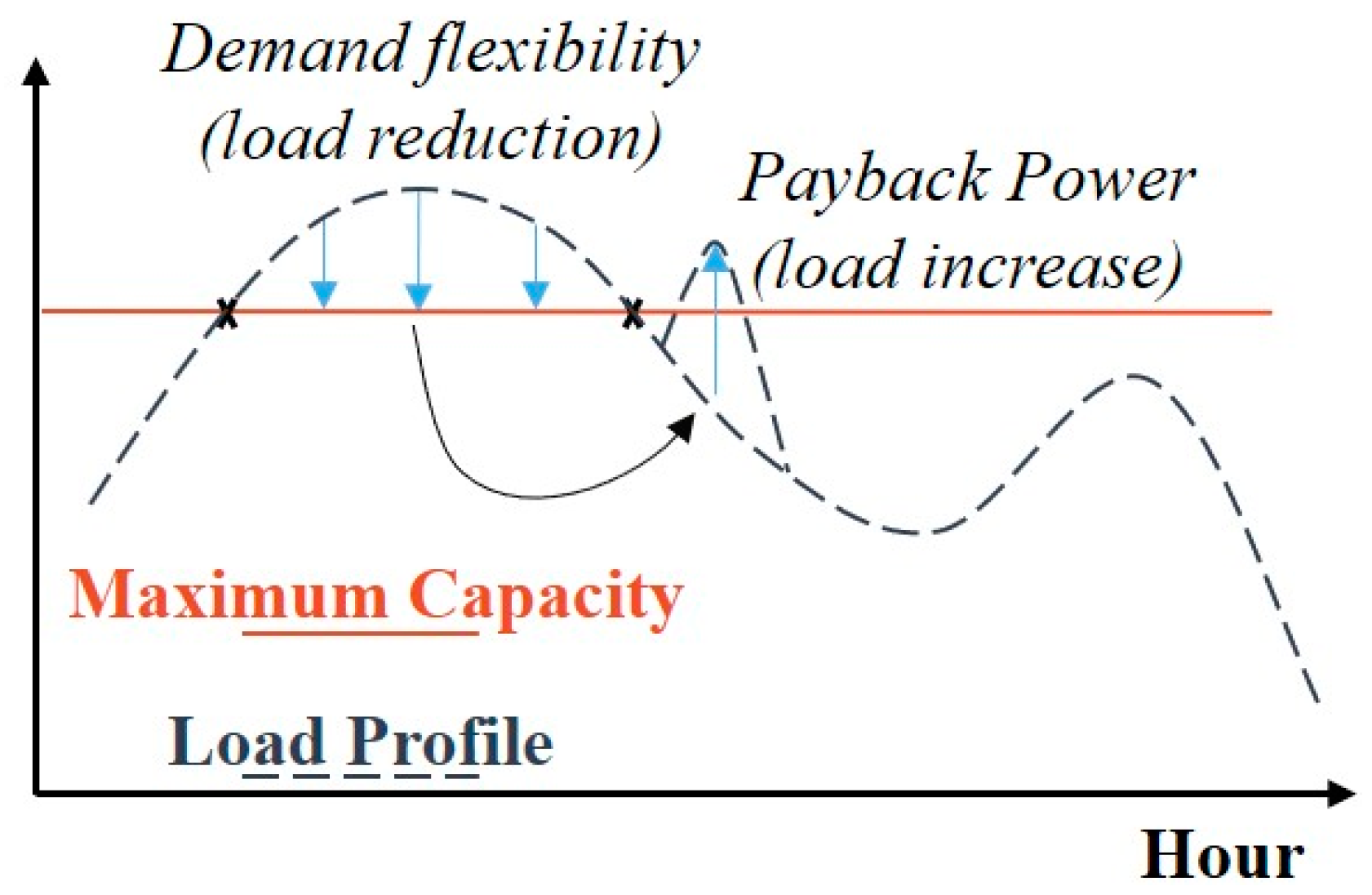
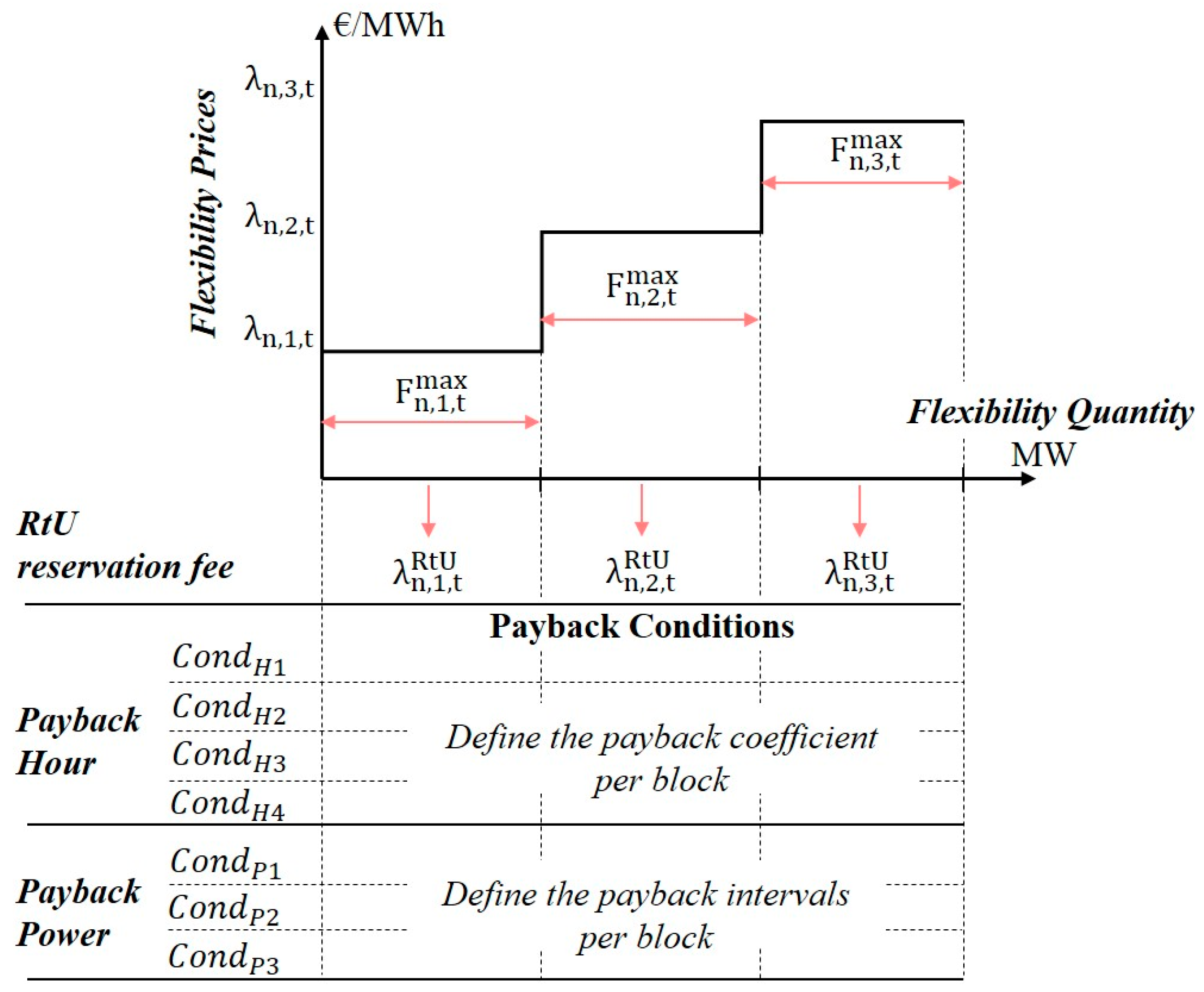
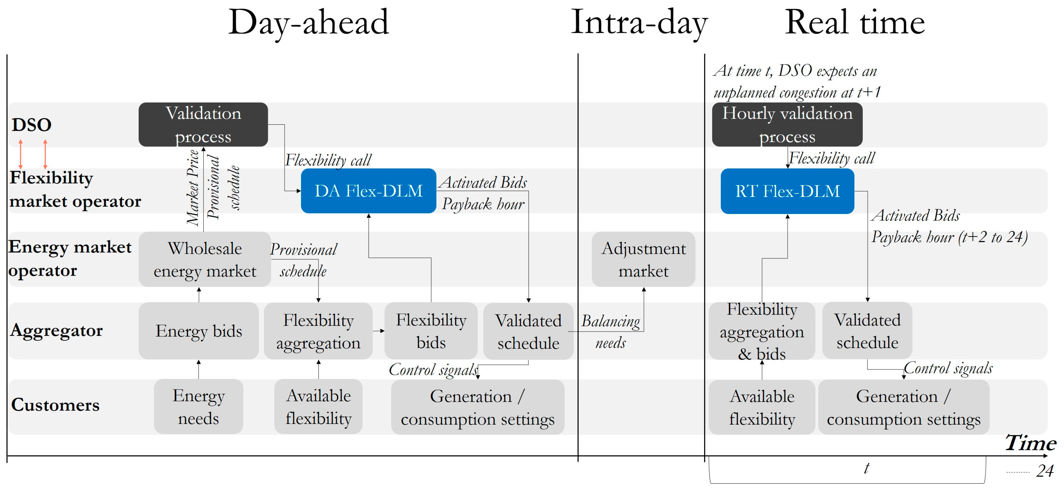
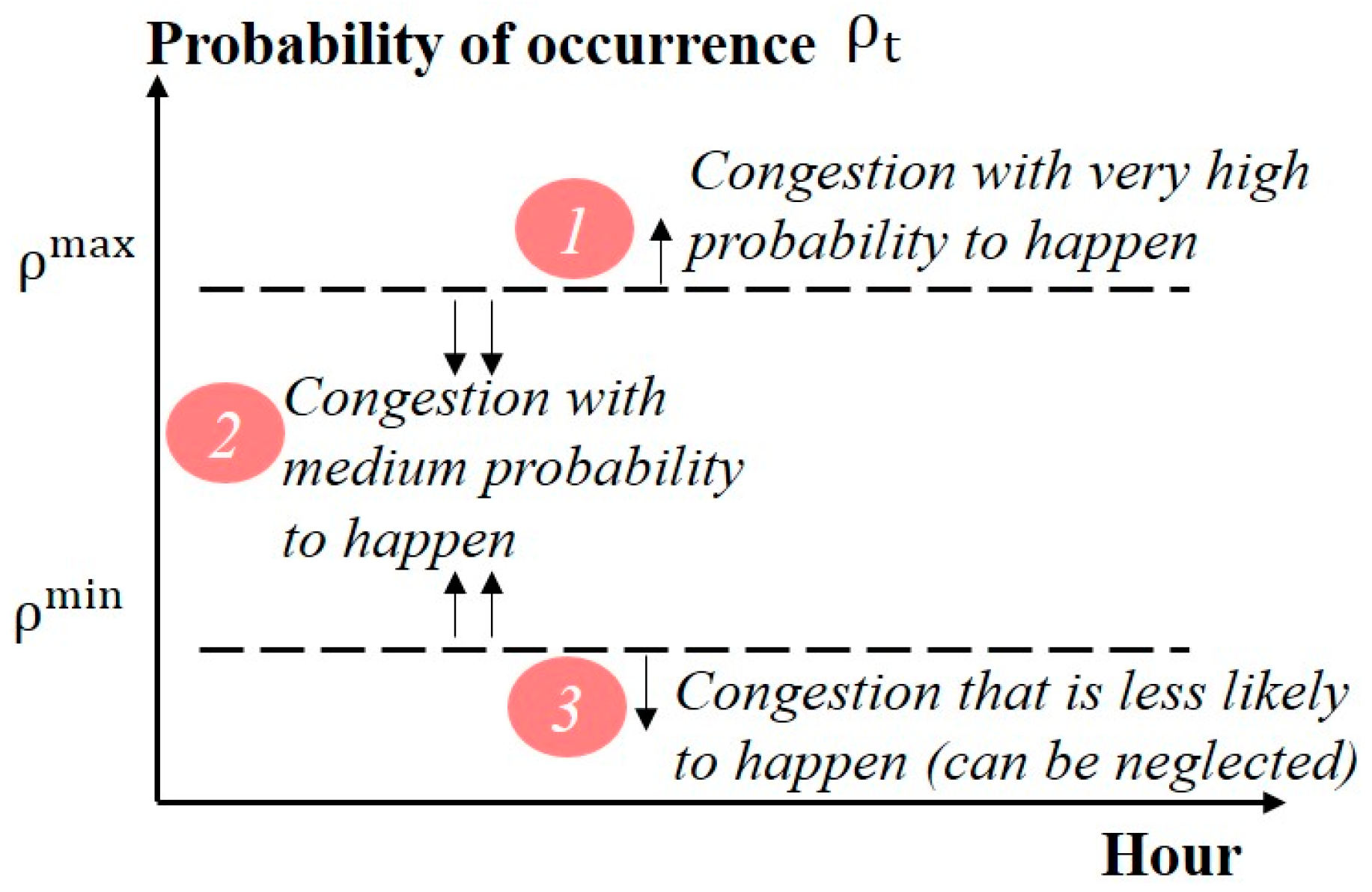
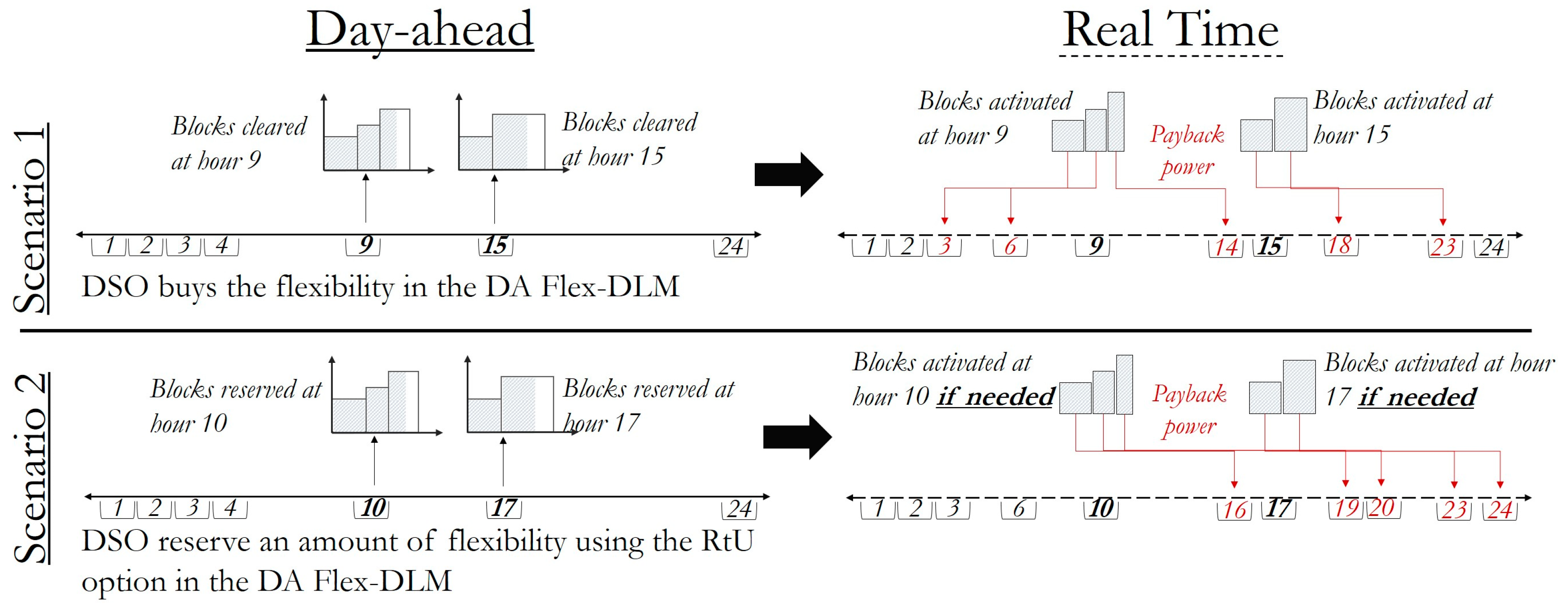
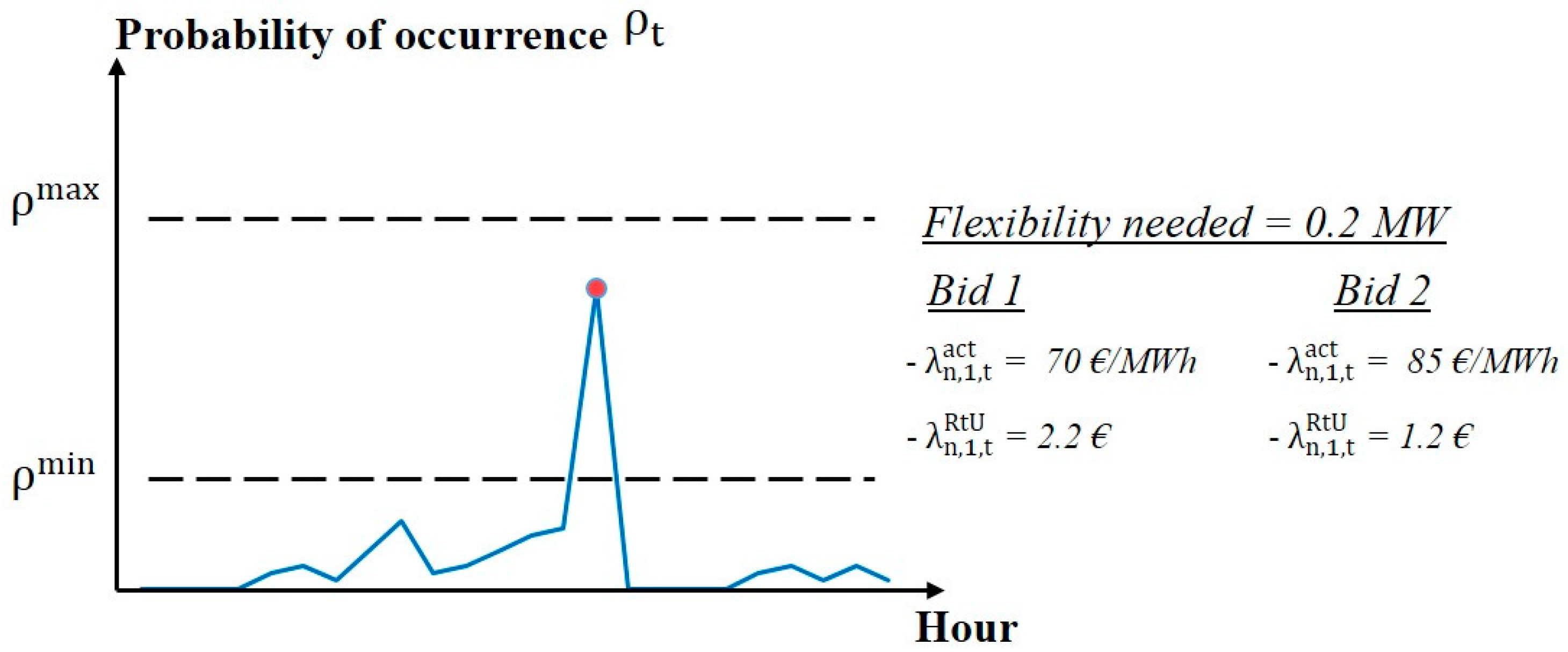
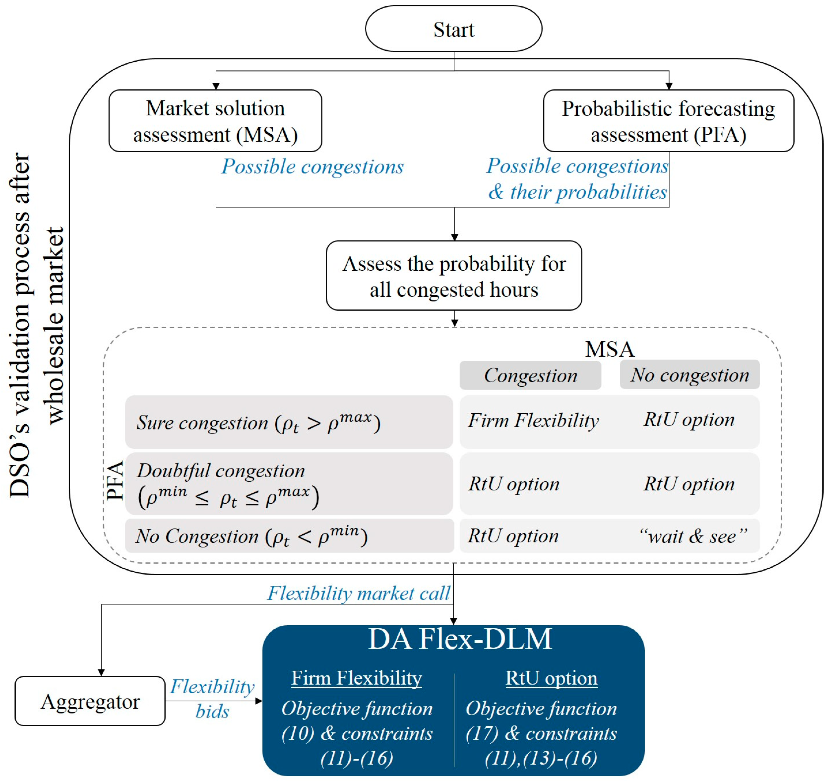
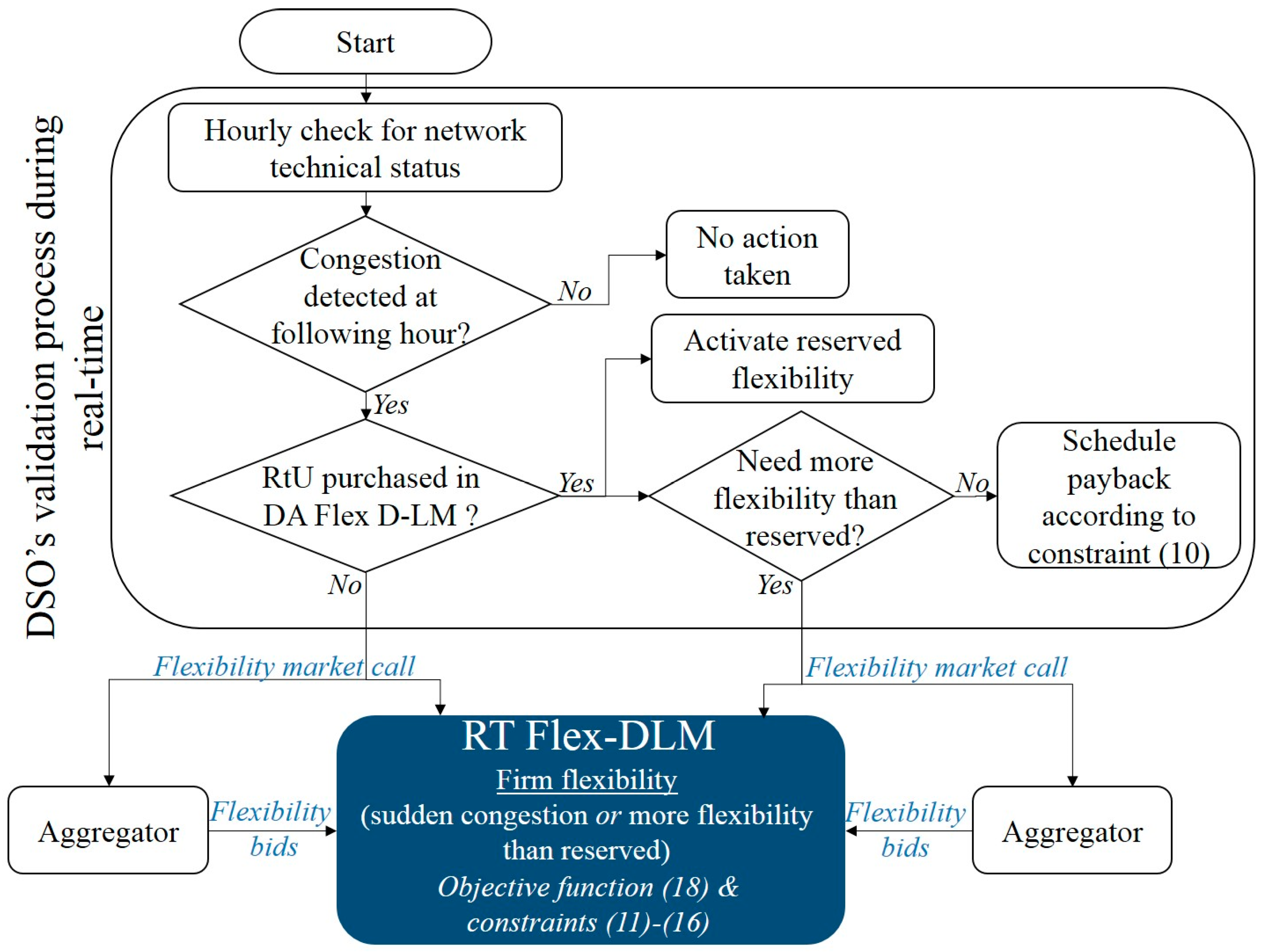
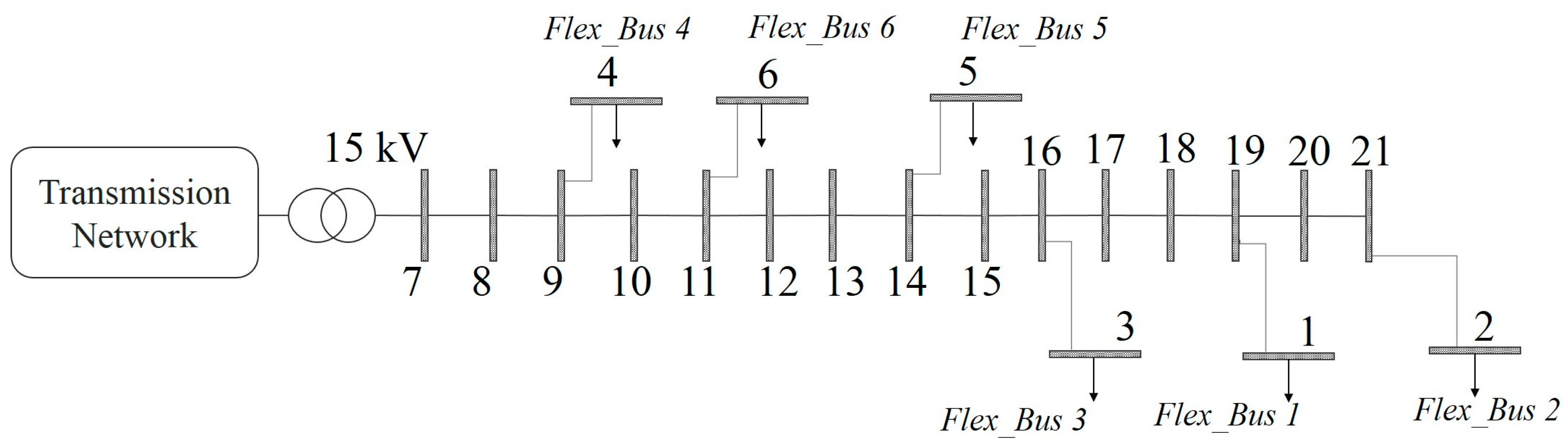
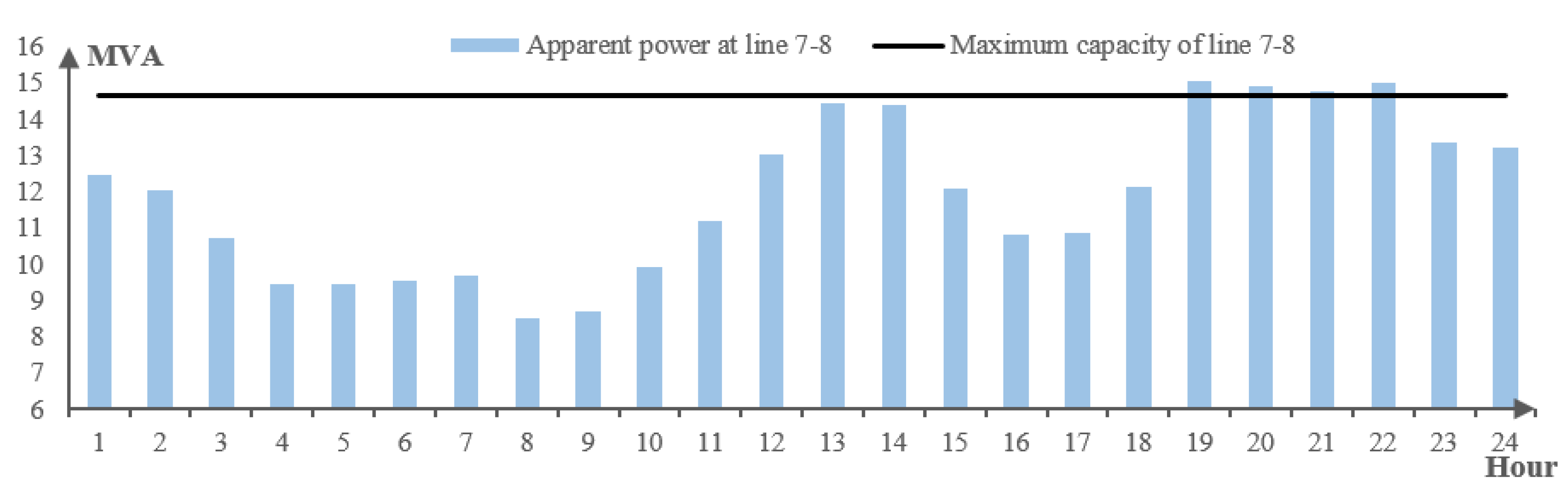
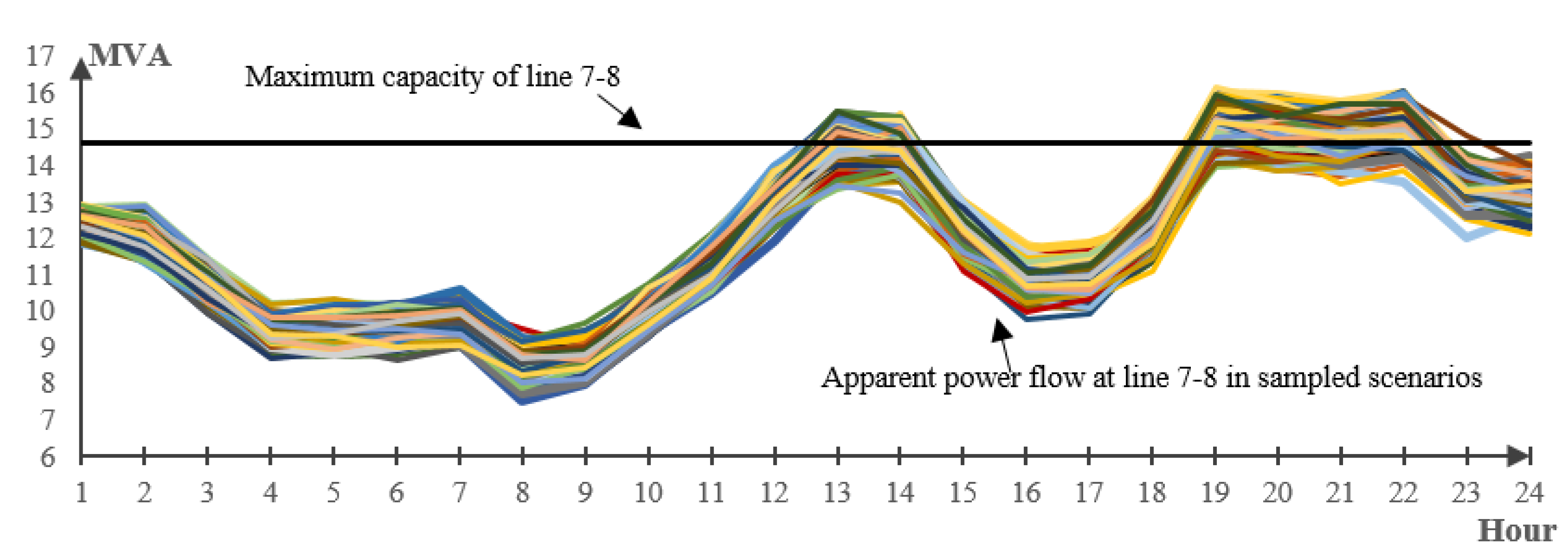
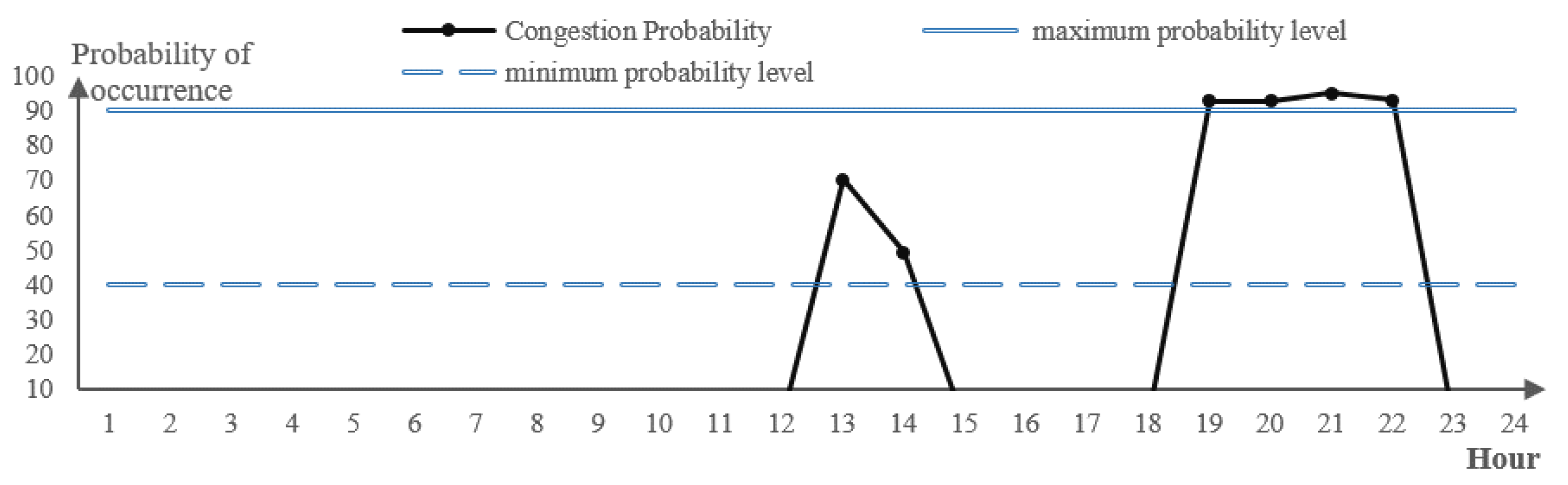
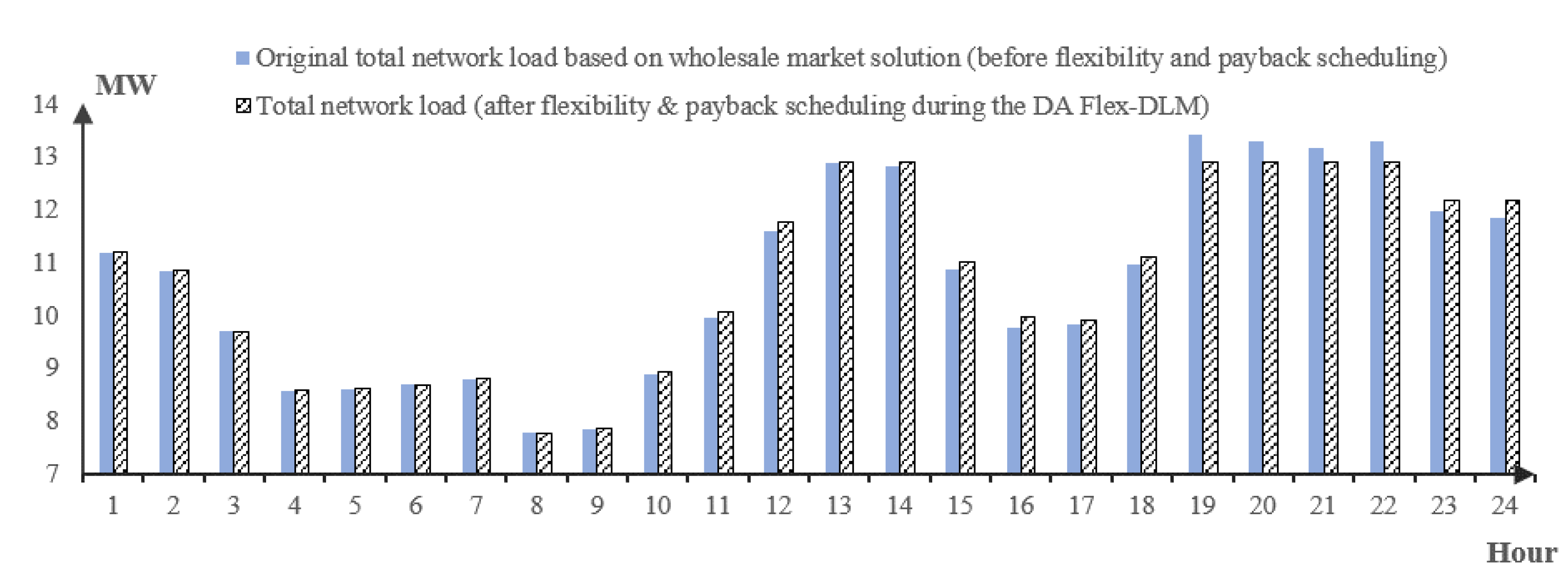
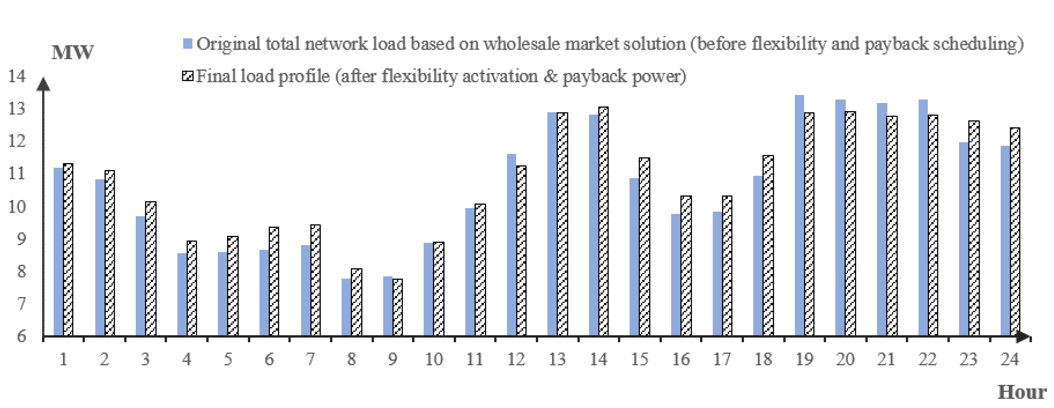
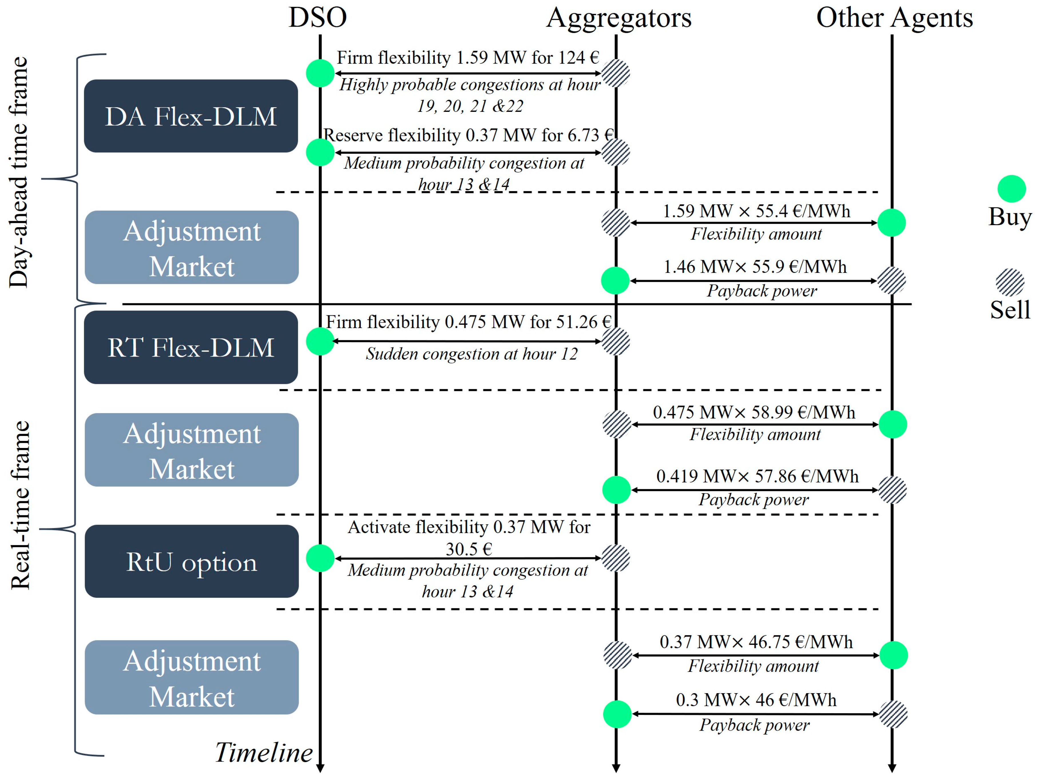
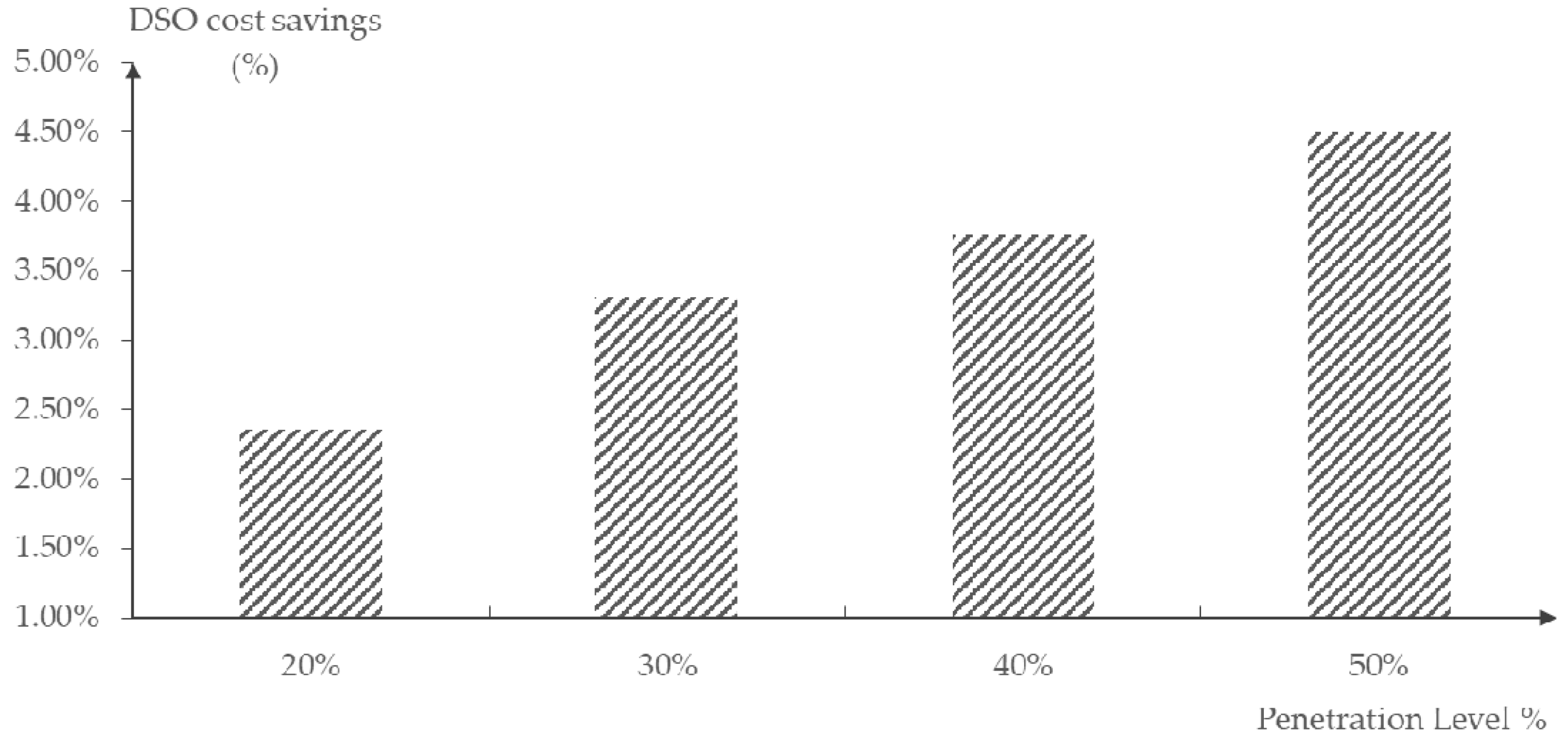
Table 1.
Summary for literature with respect to research gaps.
| Ref | The Payback Effect | The Grid Constraints | Complementary Trading Processes | Uncertainty of Demand |
|---|---|---|---|---|
| [17] | ||||
| [18] | ||||
| [19] | ||||
| [20,21] | ||||
| [22] | ||||
| [23,24] | ||||
| [25] | ||||
| [26,27] |
Table 2.
Payback conditions.
| Payback Conditions | Type | Description |
|---|---|---|
| Payback Hour | Payback power must be on following hour of flexibility activation. | |
| Payback power is in between a predefined time interval (before or after flexibility activation). | ||
| Payback power can be at any hour during the day. | ||
| Payback power is not needed. | ||
| Payback Power | Payback power is equal to the flexibility activated. | |
| Payback power is a factor of the flexibility activated. | ||
| Payback power is not needed. |
Table 3.
Possible DSO’s strategy for buying flexibility services in the DA Flex-DLM.
| Indicator | MSA | ||
|---|---|---|---|
| Congestion | No Congestion | ||
| PFA | Sure congestion | Firm flexibility | RtU option |
| Unsure congestion | RtU option | RtU option | |
| No Congestion | RtU option | “wait-and-see” | |
Table 4.
Example for the cost of reserving 0.2 MW from two bids considering different probabilities of congestion occurrence.
Table 4.
Example for the cost of reserving 0.2 MW from two bids considering different probabilities of congestion occurrence.
| Bids | Bid 1 | Bid 2 | Bid 1 | Bid 2 | Bid 1 | Bid 2 | Bid 1 | Bid 2 |
|---|---|---|---|---|---|---|---|---|
| 0.3 | 0.5 | 0.8 | No Probability Considered | |||||
| (€/MWh) | 70 | 85 | 70 | 85 | 70 | 85 | 70 | 85 |
| (€) | 2.2 | 1.2 | 2.2 | 1.2 | 2.2 | 1.2 | 2.2 | 1.2 |
| (€) | 6.4 | 6.3 | 9.2 | 9.7 | 13.4 | 14.8 | 16.2 | 18.2 |
Table 5.
Flexibility bids at buses 1, 2 & 3 in the DA Flex-DLM for high probability congestions.
| Hour | Flex_Bus 1 | Flex_Bus 2 | Flex_Bus 3 | |||||||||
|---|---|---|---|---|---|---|---|---|---|---|---|---|
| MW | €/MWh | MW | MW | MW | €/MWh | €/MWh | €/MWh | MW | MW | €/MWh | €/MWh | |
| 19 | 0.123 | 76.82 | 0.036 | 0.051 | 0.015 | 73.80 | 76.06 | 77.57 | 0.022 | 0.065 | 72.29 | 76.06 |
| 20 | 0.125 | 80.78 | 0.038 | 0.054 | 0.016 | 77.60 | 79.98 | 81.57 | 0.023 | 0.069 | 76.02 | 79.98 |
| 21 | 0.120 | 83.00 | 0.036 | 0.052 | 0.016 | 79.74 | 82.19 | 83.82 | 0.022 | 0.067 | 78.11 | 82.19 |
| 22 | 0.125 | 79.98 | 0.039 | 0.056 | 0.017 | 76.84 | 79.20 | 80.77 | 0.024 | 0.072 | 75.27 | 79.20 |
| 0.85 | - | 0.80 | 0.95 | 0.70 | - | 0.82 | 0.95 | - | ||||
| Payback hour | 1–24 | - | 13–24 | 1–16 | 17–24 | - | 12–20 | 6–16 | - | |||
Table 6.
Flexibility bids at buses 4, 5 & 6 in the DA Flex-DLM for high probability congestions.
| Hour | Flex_Bus 4 | Flex_Bus 5 | Flex_Bus 6 | |||||||||||
|---|---|---|---|---|---|---|---|---|---|---|---|---|---|---|
| MW | MW | MW | €/MWh | €/MWh | €/MWh | MW | MW | €/MWh | €/MWh | MW | MW | €/MWh | €/MWh | |
| 19 | 0.030 | 0.050 | 0.020 | 72.29 | 73.80 | 78.33 | 0.066 | 0.054 | 76.82 | 77.57 | 0.035 | 0.065 | 76.06 | 76.82 |
| 20 | 0.027 | 0.045 | 0.018 | 76.02 | 77.60 | 82.36 | 0.060 | 0.049 | 80.78 | 81.57 | 0.032 | 0.059 | 79.98 | 80.78 |
| 21 | 0.026 | 0.044 | 0.018 | 78.11 | 79.74 | 84.63 | 0.058 | 0.047 | 83.00 | 83.82 | 0.031 | 0.057 | 82.19 | 83.00 |
| 22 | 0.027 | 0.045 | 0.018 | 75.27 | 76.84 | 81.55 | 0.059 | 0.049 | 79.98 | 80.77 | 0.032 | 0.059 | 79.20 | 79.98 |
| 0.90 | 0.95 | 0.80 | - | 0.88 | 0.92 | - | 0.94 | 1.00 | - | |||||
| Payback hour | 8–13 | 9–18 | 1–24 | - | 1–24 | 12–16 | - | 1–24 | 1–24 | - | ||||
Table 7.
Market solution for DA Flex-DLM for the highly probable congestions.
| Flex_Bus 1 | Flex_Bus 2 | Flex_Bus 3 | Flex_Bus 4 | Flex_Bus 5 | Flex_Bus 6 | |||||||||
|---|---|---|---|---|---|---|---|---|---|---|---|---|---|---|
| Firm Flexibility (MW) | ||||||||||||||
| Hour | 19 | 0.123 | 0.036 | 0.051 | - | 0.022 | 0.065 | 0.030 | 0.050 | - | 0.066 | - | 0.035 | 0.056 |
| 20 | - | 0.038 | 0.054 | - | 0.023 | 0.069 | 0.027 | 0.045 | - | 0.060 | - | 0.032 | 0.043 | |
| 21 | - | 0.036 | 0.052 | - | 0.022 | 0.067 | 0.026 | 0.044 | - | - | - | 0.022 | - | |
| 22 | - | 0.039 | 0.056 | - | 0.024 | 0.072 | 0.027 | 0.045 | - | 0.039 | - | 0.032 | 0.059 | |
| Payback power (MW) | ||||||||||||||
| Hour | 9 | - | - | - | - | - | - | 0.020 | - | - | - | - | - | - |
| 10 | - | - | - | - | - | - | 0.030 | - | - | - | - | - | - | |
| 11 | - | - | 0.035 | - | - | 0.044 | 0.030 | - | - | - | - | - | - | |
| 12 | - | - | 0.056 | - | - | 0.072 | 0.030 | - | - | - | - | - | - | |
| 13 | - | - | - | - | 0.006 | - | - | - | - | - | - | - | - | |
| 14 | - | 0.039 | - | - | 0.024 | - | - | - | - | - | - | - | - | |
| 15 | - | - | 0.056 | - | - | 0.072 | - | 0.025 | - | - | - | - | - | |
| 16 | - | - | 0.056 | - | - | 0.072 | - | 0.050 | - | - | - | - | - | |
| 17 | - | - | - | - | 0.021 | - | - | 0.050 | - | - | - | 0.009 | - | |
| 18 | - | 0.002 | - | - | 0.024 | - | - | 0.050 | - | 0.013 | - | 0.035 | 0.028 | |
| 23 | - | 0.039 | - | - | - | - | - | - | - | 0.066 | - | 0.035 | 0.065 | |
| 24 | 0.104 | 0.039 | - | - | - | - | - | - | - | 0.066 | - | 0.035 | 0.065 | |
| (€) | 124 | |||||||||||||
Table 8.
Flexibility bids at buses 2, 4 & 6 in the DA Flex-DLM for medium probability congestions.
| Hour | Flex_Bus 2 | Flex_Bus 4 | Flex_Bus 6 | |||||||||||||
|---|---|---|---|---|---|---|---|---|---|---|---|---|---|---|---|---|
| MW | MW | MW | €/MWh | €/MWh | €/MWh | MW | MW | MW | €/MWh | €/MWh | €/MWh | MW | MW | €/MWh | €/MWh | |
| 13 | 0.046 | 0.053 | 0.020 | 85.22 | 85.50 | 85.68 | 0.035 | 0.042 | 0.037 | 85.04 | 85.22 | 85.77 | 0.041 | 0.060 | 85.50 | 85.59 |
| 14 | 0.046 | 0.052 | 0.020 | 89.40 | 89.68 | 89.87 | 0.034 | 0.041 | 0.036 | 89.21 | 89.40 | 89.97 | 0.039 | 0.058 | 89.68 | 89.78 |
| (€) | - | 0.78 | 0.90 | 0.34 | - | 0.59 | 0.72 | 0.64 | - | 0.69 | 1.02 | |||||
| (€) | - | 0.82 | 0.94 | 0.35 | - | 0.60 | 0.73 | 0.65 | - | 0.71 | 1.04 | |||||
Table 9.
Market solution for DA Flex-DLM for the medium probability congestions.
| Flex_Bus 2 | Flex_Bus 4 | Flex_Bus 6 | |||||||
|---|---|---|---|---|---|---|---|---|---|
| Flexibility Reserved (MW) | |||||||||
| Hour | 13 | 0.047 | 0.054 | 0.020 | 0.035 | 0.042 | - | 0.024 | - |
| 14 | 0.046 | 0.052 | 0.020 | 0.034 | - | - | - | - | |
| Reservation cost (€) | 6.73 | ||||||||
Table 10.
Flexibility bids at buses 1, 2 & 3 in the RT Flex-DLM for sudden congestions.
| Hour | Flex_Bus 1 | Flex_Bus 2 | Flex_Bus 3 | |||||||||
|---|---|---|---|---|---|---|---|---|---|---|---|---|
| MW | €/MWh | MW | MW | MW | €/MWh | €/MWh | €/MWh | MW | MW | €/MWh | €/MWh | |
| 12 | 0.081 | 108.61 | 0.052 | 0.074 | 0.022 | 106.89 | 108.18 | 109.04 | 0.028 | 0.085 | 106.03 | 108.18 |
| 0.85 | - | 0.80 | 0.95 | 0.70 | - | 0.82 | 0.95 | - | ||||
| Payback hour | 10–24 | - | 13–24 | 10–16 | 17–24 | - | 12–20 | 10–16 | - | |||
Table 11.
Flexibility bids at buses 4, 5 & 6 in the RT Flex-DLM for sudden congestions.
| Hour | Flex_Bus 4 | Flex_Bus 5 | Flex_Bus 6 | |||||||||||
|---|---|---|---|---|---|---|---|---|---|---|---|---|---|---|
| MW | MW | MW | €/MWh | €/MWh | €/MWh | MW | MW | €/MWh | €/MWh | MW | MW | €/MWh | €/MWh | |
| 12 | 0.031 | 0.052 | 0.021 | 106.03 | 106.89 | 109.46 | 0.051 | 0.042 | 108.61 | 109.04 | 0.024 | 0.045 | 108.18 | 108.61 |
| 0.90 | 0.95 | 0.80 | - | 0.88 | 0.92 | - | 0.94 | 1.00 | - | |||||
| Payback hour | 10–13 | 10–18 | 10–24 | - | 10–24 | 12–16 | - | 10–24 | 10–24 | - | ||||
Table 12.
Market solution for RT Flex-DLM for a sudden congestion at hour 12.
| Flex_Bus 1 | Flex_Bus 2 | Flex_Bus 3 | Flex_Bus 4 | Flex_Bus 5 | Flex_Bus 6 | |||||||||
|---|---|---|---|---|---|---|---|---|---|---|---|---|---|---|
| Firm Flexibility (MW) | ||||||||||||||
| Hour | 12 | 0.062 | 0.052 | 0.074 | - | 0.028 | 0.085 | - | 0.052 | - | 0.051 | - | 0.024 | 0.045 |
| Payback power (MW) | ||||||||||||||
| Hour | 16 | - | - | - | - | - | 0.081 | - | - | - | - | - | - | - |
| 17 | - | - | - | - | - | - | - | - | - | - | - | - | - | |
| 18 | 0.053 | 0.041 | 0.070 | - | - | - | - | 0.050 | - | 0.045 | - | 0.023 | 0.045 | |
| 20 | - | - | - | - | 0.023 | - | - | - | - | - | - | - | - | |
| (€) | 51.26 | |||||||||||||
Table 13.
Payback hours for activated flexibility bids reserved by the RtU option for hours 13 and 14.
Table 13.
Payback hours for activated flexibility bids reserved by the RtU option for hours 13 and 14.
| Flex_Bus 2 | Flex_Bus 4 | Flex_Bus 6 | |||||||
|---|---|---|---|---|---|---|---|---|---|
| Payback Power (MW) | |||||||||
| Hour | 17 | 0.038 | 0.043 | 0.016 | 0.028 | 0.034 | - | 0.019 | - |
| 18 | 0.037 | 0.042 | 0.016 | 0.027 | - | - | - | - | |
| Activation cost (€) | 30.5 | ||||||||
| (€) | 37.23 | ||||||||
Table 14.
Activated flexibility at buses with respect to penetration levels of flexibility.
| Flexibility Penetration Level | Flex_Bus 1 | Flex_Bus 2 | Flex_Bus 3 | Flex_Bus 4 | Flex_Bus 5 | Flex_Bus 6 |
|---|---|---|---|---|---|---|
| MW | MW | MW | MW | MW | MW | |
| 10% | 0.123 | 0.362 | 0.365 | 0.295 | 0.165 | 0.279 |
| 20% | 0 | 0.519 | 0.270 | 0.590 | 0 | 0.209 |
| 30% | 0 | 0.450 | 0.274 | 0.759 | 0 | 0.105 |
| 40% | 0 | 0.391 | 0.365 | 0.832 | 0 | 0 |
| 50% | 0 | 0.482 | 0.457 | 0.650 | 0 | 0 |
© 2018 by the authors. Licensee MDPI, Basel, Switzerland. This article is an open access article distributed under the terms and conditions of the Creative Commons Attribution (CC BY) license (http://creativecommons.org/licenses/by/4.0/).
Share and Cite
MDPI and ACS Style
Esmat, A.; Usaola, J.; Moreno, M.Á. A Decentralized Local Flexibility Market Considering the Uncertainty of Demand. Energies 2018, 11, 2078. https://0-doi-org.brum.beds.ac.uk/10.3390/en11082078
AMA Style
Esmat A, Usaola J, Moreno MÁ. A Decentralized Local Flexibility Market Considering the Uncertainty of Demand. Energies. 2018; 11(8):2078. https://0-doi-org.brum.beds.ac.uk/10.3390/en11082078
Chicago/Turabian StyleEsmat, Ayman, Julio Usaola, and Mª Ángeles Moreno. 2018. "A Decentralized Local Flexibility Market Considering the Uncertainty of Demand" Energies 11, no. 8: 2078. https://0-doi-org.brum.beds.ac.uk/10.3390/en11082078
Note that from the first issue of 2016, this journal uses article numbers instead of page numbers. See further details here.