A Short-Term Wind Speed Forecasting Model by Using Artificial Neural Networks with Stochastic Optimization for Renewable Energy Systems


1
School of Electrical Engineering and Automation, Jiangxi University of Science and Technology, Ganzhou 341000, Jiangxi, China
2
Computer and Intelligent Robot Program for Bachelor Degree, National Pingtung University, Pingtung 90004, Taiwan
*
Author to whom correspondence should be addressed.
Energies 2018, 11(10), 2777; https://0-doi-org.brum.beds.ac.uk/10.3390/en11102777
Submission received: 30 September 2018
/
Revised: 9 October 2018
/
Accepted: 10 October 2018
/
Published: 16 October 2018
(This article belongs to the Special Issue Energy Economy, Sustainable Energy and Energy Saving)
Abstract
:To efficiently manage unstable wind power generation, precise short-term wind speed forecasting is critical. To overcome the challenges in wind speed forecasting, this paper proposes a new convolutional neural network algorithm for short-term forecasting. In this paper, the forecasting performance of the proposed algorithm was compared to that of four other artificial intelligence algorithms commonly used in wind speed forecasting. Numerical testing results based on data from a designated wind site in Taiwan were used to demonstrate the efficiency of above-mentioned proposed learning method. Mean absolute error (MAE) and root-mean-square error (RMSE) were adopted as accuracy evaluation indexes in this paper. Experimental results indicate that the MAE and RMSE values of the proposed algorithm are 0.800227 and 0.999978, respectively, demonstrating very high forecasting accuracy.
1. Introduction
The depletion of fossil fuels, increased environmental pollution and the development and maximum utilization of renewable energy sources have attracted the attention of experts and scholars globally [1,2,3]. Sustainability transitions are long-term, multi-dimensional, and fundamental transformation processes [4], and it is also one of the greatest challenges in the 21st century [5]. As a non-polluting renewable energy source, wind energy is highly valued by many countries. Wind power generation has emerged as one of the most mature renewable energy power generation technologies including high commercialization potential [6].
In aspect of the prices time series problem [7,8,9], Cincotti et al., used the three different methods to the model this issue: a discrete-time univariate econometric model and two artificial intelligence techniques. Support vector machine (SVM) methodology gives better forecasting accuracy for price time series [8]. However, this paper proposes that the performance of WindNet compared to that of SVM, random forest (RF), decision tree (DT), multilayer perceptron (MLP), convolutional neural network CNN, and long short-term memory (LSTM) architectures is the best in that its average MAE and RMSE values are the lowest.
Short-term wind speed prediction of wind farms is one of the most effective ways to solve the above-mentioned energy problems. This corresponds to the effective prediction of the wind speed and the wind farm power output, according to the power curve of the wind turbine. This enables the power dispatch system to adjust the dispatch schedule in time, according to changes in wind power output. This ensures power quality, reduces power system reserve capacity and lowers power system operation cost. Effective prediction will also improve wind power penetration rate and reduce the impact of wind power on the power grid. Therefore, accurate short-term wind power forecasting can reduce the risk of power grid transmission and integration [10].
According to theory, since wind speed pattern is determined by natural meteorological rules, the pattern has inherent regularity, which proves the feasibility for wind speed forecasting. However, in practice, wind speed fluctuates randomly and is unstable [11]. Different wind speeds correspond to different locations, sometimes wind speeds at the same location may differ with time, while wind speeds may also vary at the same altitude. Factors such as seasonality, temperature, humidity, air pressure and other parameters have to be considered [12]. Therefore, there are still significant obstacles in wind speed forecasting.
Renewable energy issues has recently attracted much attention, thus there have been many studies on wind speed forecasting [13]. According to [14] a Bayesian structural break model was proposed to conduct exact short-term wind speed forecasting. The experiment testing data is actual data collected from utility scale wind turbines. The experiment also applied mean absolute error (MAE), mean square error (MSE) and root mean square error (RMSE) for performance evaluation. Furthermore, the experiment could also be applied in applications such as wind turbine predictive control and wind power scheduling. The precision of this method is very high, but it is only suitable for ultra-short wind speed predictions of a few seconds to a few hours. Authors [15] proposed a wind speed and solar radiation co-testing system based on extreme learning machines (ELM) and principal components analysis (PCA). According to literature [15], PCA can be used to reduce data dimension, since this approach can greatly reduce the complexity of model training. The experiment also proved that while maintaining forecasting accuracy, ELM model training is significantly faster compared to (a) multi-layer perceptron network, (b) radial basis function networks and (c) least squares support vector machines. However, this method is applicable exclusively for short-term wind speed forecasting (few hours) and not for long-term predictions. Wang et al. [16], integrated various multi-step-ahead wind speed forecasting models and furthermore compared and analyzed each model. They further mentioned that multi-step-ahead prediction of wind speed is very challenging and that this goal can be achieved by adopting the weather research and forecasting (WRF) model. In addition, they also mentioned that multiple strategies are more effective than single strategies in the research of wind speed prediction. The integration of various models to construct a combination of direct and multi-input multi-output strategies (COMB-DIRMOs) corresponds to a practical, effective and robust model.
Currently there are many studies related to wind speed-forecasting methods and each method has its own advantages and disadvantages. Therefore, many experts and scholars use ensemble methods to predict wind speed [17]. Ensemble methods can be divided into two major types: competitive ensemble forecasting and cooperative ensemble forecasting. Ren et al. [17], compared and proposed improvements on the most current state-of-the-art wind speed prediction ensemble methods. Jiang et al. [18], combined v-support vector machine (v-SVM) and cuckoo search (CS) to conduct short-term wind speed forecasting. In this method, CS is used to adjust the parameters of v-SVM and the experimental results proved that the performance of CS is improved compared to that of particle swarm optimization (PSO). Zhang et al. [19], integrated three different methods to predict wind speed: the ensemble empirical mode decomposition (EEMD), adaptive neural network-based fuzzy inference system (ANFIS) and seasonal auto-regression integrated moving average (SARIMA). Jiang et al. [18] and Zhang et al. [19] both proposed hybrid wind speed prediction models that present an adequate prediction performance. Nevertheless, both studies present predictive wind speed results within a few hours period and are not applicable for long term wind speed analysis.
As it concerns neural network wind speed prediction, More and Deo [20] proposed a basic neural network architecture to conduct wind speed prediction and its feasibility was experimentally confirmed. However, there are various kinds of neural network architectures and there are several variants concerning even the most basic neural networks. The most basic neural network architecture was presented by Li and Shi [21]. Prediction comparisons were conducted between three different models (adaptive linear element, back propagation and radial basis function). The result of the research indicated that these three methods include advantages and disadvantages. Thus, the selection of a neural network model is a significant issue. Guo et al. [22], proposed a multi-step forecasting model to achieve wind speed prediction. This method applied the empirical mode decomposition (EMD) neural network, which corresponds to the use of a number of traditional neural networks to predict wind speed. Although this method has been proven effective during experiments, the parameters of neural networks that need to be trained further increased. Hence, the complexity of the training may increase significantly. However, with the development of deep learning technology, the convolutional neural network (CNN) architecture adopted in this paper not only differentiates among various machine-learning algorithms, but also additionally predicts wind speed for a 3 day-period including the highest accuracy. Hence, this provides to the energy management systems the most precise and efficient power dispatching.
The major contributions of this paper include: (a) The development of a powerful wind speed-forecasting algorithm for renewable energy systems; (b) Comparison of the performances of the several popular machine learning methods on the challenge of wind speed forecasting and (c) Demonstration of the feasibility and practicality of the proposed model as a significant wind speed forecasting application.
This paper is organized as follows: Section 2 reviews the variety of renewable resource forecasting techniques. Section 3 introduces the proposed CNN model. Section 4 illustrates the wind speed forecasting results of the proposed model and the comparison results between the proposed model and current methods. Discussions are mentioned in Section 5. Finally, Section 6 concludes the experimental results of this paper.
2. Renewable Resource Forecasting Techniques Overview
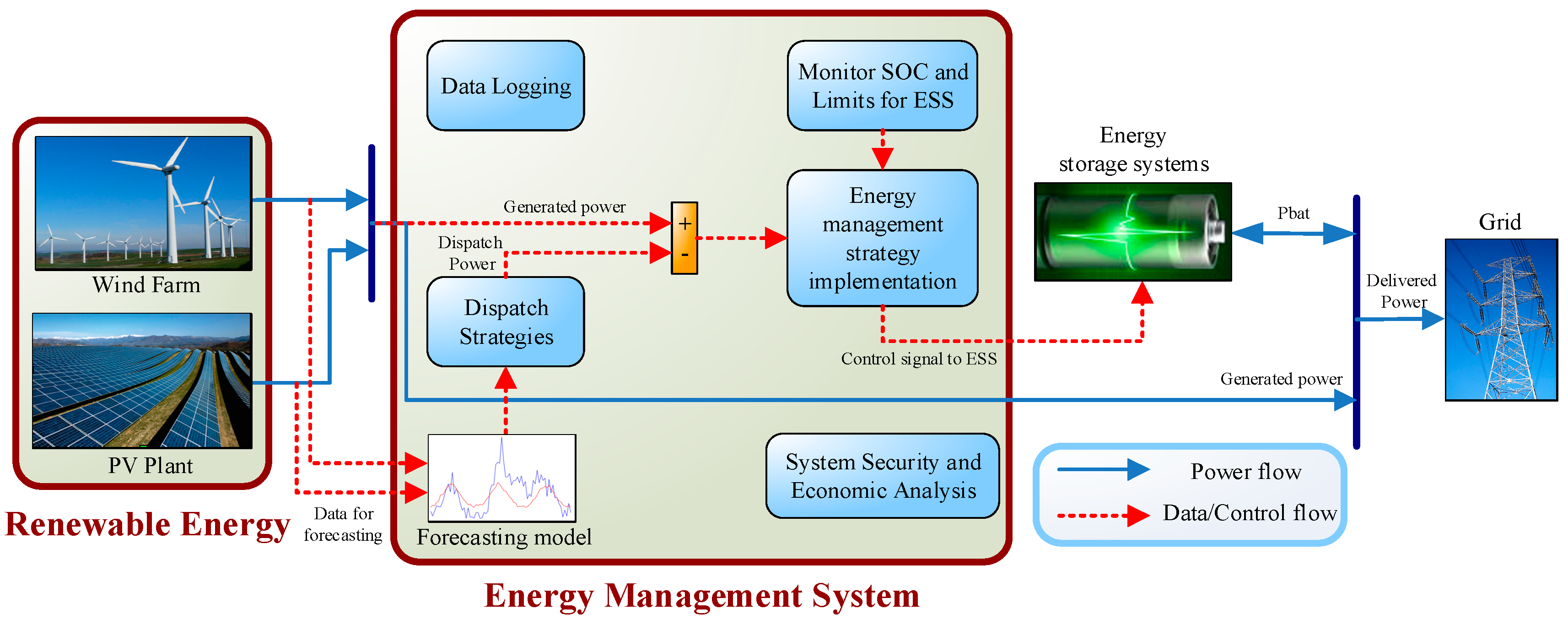
Figure 1 illustrates the architecture of a renewable energy management system [23]. The energy management system (EMS) addresses issues of energy control, management, maintenance, and consumption, to assist in the electrical equipment maintenance and repair within the factory, farm, or even a whole city. It can monitor the operation status of the equipment and improve overall management immediately. Good management practices can extend the life of electrical equipment and reduce costs. In the event of equipment failures or various other conditions, the system can immediately send out an alarm to facilitate management personnel monitoring and maintenance and thus losses are decreased to minimum. In the case of aging intensive energy-demanding devices, the EMS can also notify management personnel to proceed to a replacement. In the renewable energy management system, the EMS can use programmed control system technology, network communication technology and database technology, to connect renewable energy data collection, monitoring stations and management and control centers distributed on the site to achieve data collection, storage, processing, statistics, query and analysis, and even data monitoring, and diagnosis.
Based on Figure 1, it is demonstrated that the EMS dispatches renewable energy generated power following a power prediction through the forecasting model, to achieve the goals of energy monitoring and effective management. Through centralized monitoring and effective management of energy data, energy consumption per unit is reduced and additionally economic and energy efficiency is significantly improved. Therefore, the forecasting model represents a crucial parameter in the EMS.
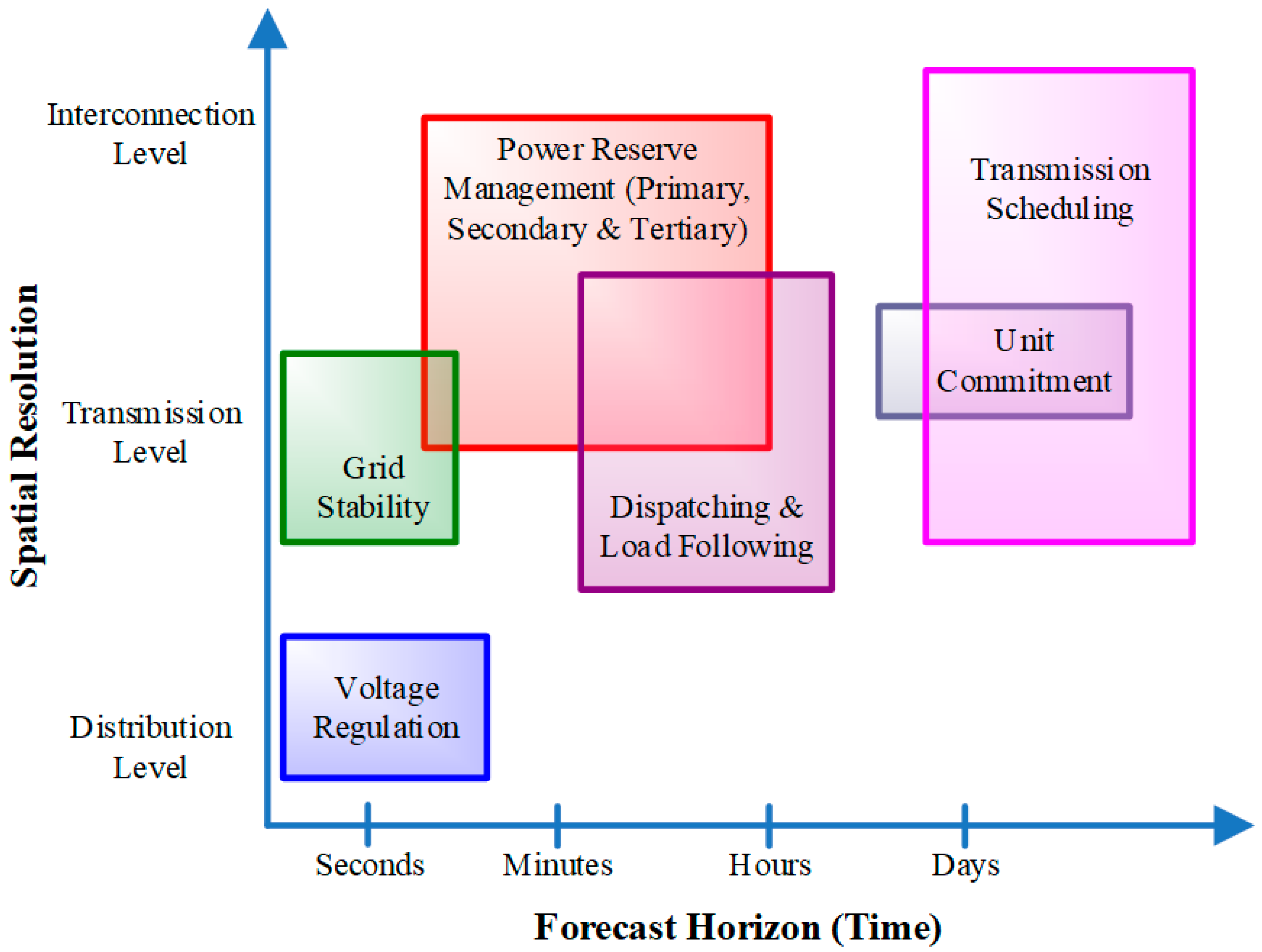
Many applications related to energy forecasting are available. Figure 2 illustrates the distribution of various applications in special resolution and forecast time coordinates. The horizontal axis of Figure 2 corresponds to the forecast horizon (time) and its resolution is divided into four different predictions of time periods: seconds, minutes, hours, and days. The vertical axis corresponds to spatial resolution, which is ordinarily divided into 3 categories: interconnection level, transmission level and distribution level. Figure 2 also lists several of the most common applications such as voltage regulation, grid stability, power reserve management (primary, secondary and tertiary), dispatching and load following, unit commitment and transmission scheduling. It is worth noting that the main focus of this paper is that dispatching and load following is positioned at the transmission level, its prediction time length, as far as current studies are concerned, mostly falls only within a few minutes to a few hours.
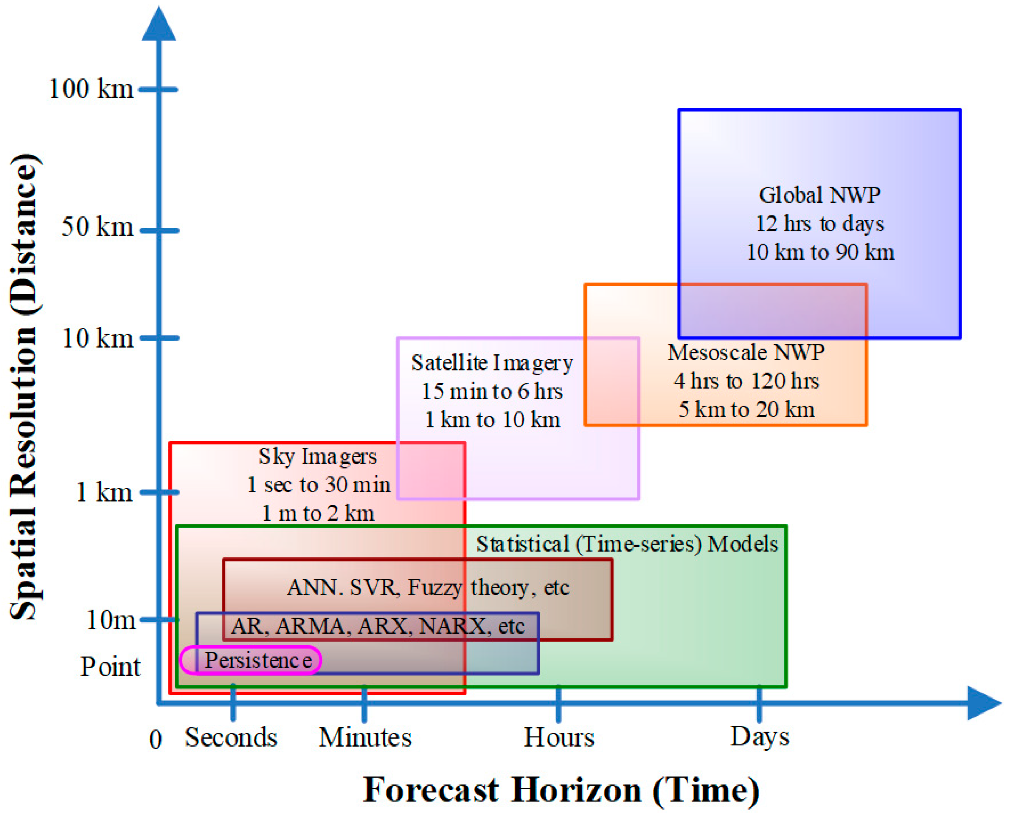
In addition, Figure 3 demonstrates the classification of different prediction methods [24]. In this figure, the vertical axis corresponds to the spatial resolution (distance) and the horizontal axis represents forecast horizon (time). Figure 3 includes a sufficient classification and description of a variety of prediction methods and models. At present, common prediction, methods include persistence, autoregressive (AR), moving average (MA), ARMA, artificial neural network (ANN), support vector regression (SVR), fuzzy theory, statistical models, sky imagers, satellite imagery, mesoscale numerical weather prediction (NWP) and global NWP. Among these methods, sky imagers fall in the interval of 1 s to 30 min and 1 m to 2 km. Satellite imagery fall between 15 min to 6 h and 1 km to 10 km. Mesoscale NWP falls between 4 h to 120 h and 5 km to 20 km. Global NWP falls between 12 h to days and 10 km to 90 km. The ANN algorithm applied in this paper, based on current research, has a prediction time length that corresponds to the period of a few seconds to several hours. Based on Figure 2 and Figure 3, it is derived that current studies on power dispatch and ANN prediction cannot achieve up to day-length forecasting results. The CNN prediction model proposed in this paper could analyze data from the past 7 days and predict wind speed conditions for the next 3 days. Hence, the EMS can accurately forecast future electricity output.
3. The Proposed CNN Model
Neural networks present powerful modeling capabilities and are widely used in many applications. In this section, authors introduce the basic multilayer perceptron (MLP) [25] and the convolutional neural network (CNN) [26,27,28,29,30,31] architecture. The WindNet algorithm proposed in this paper is also described in this chapter.
3.1. Multilayer Perceptron
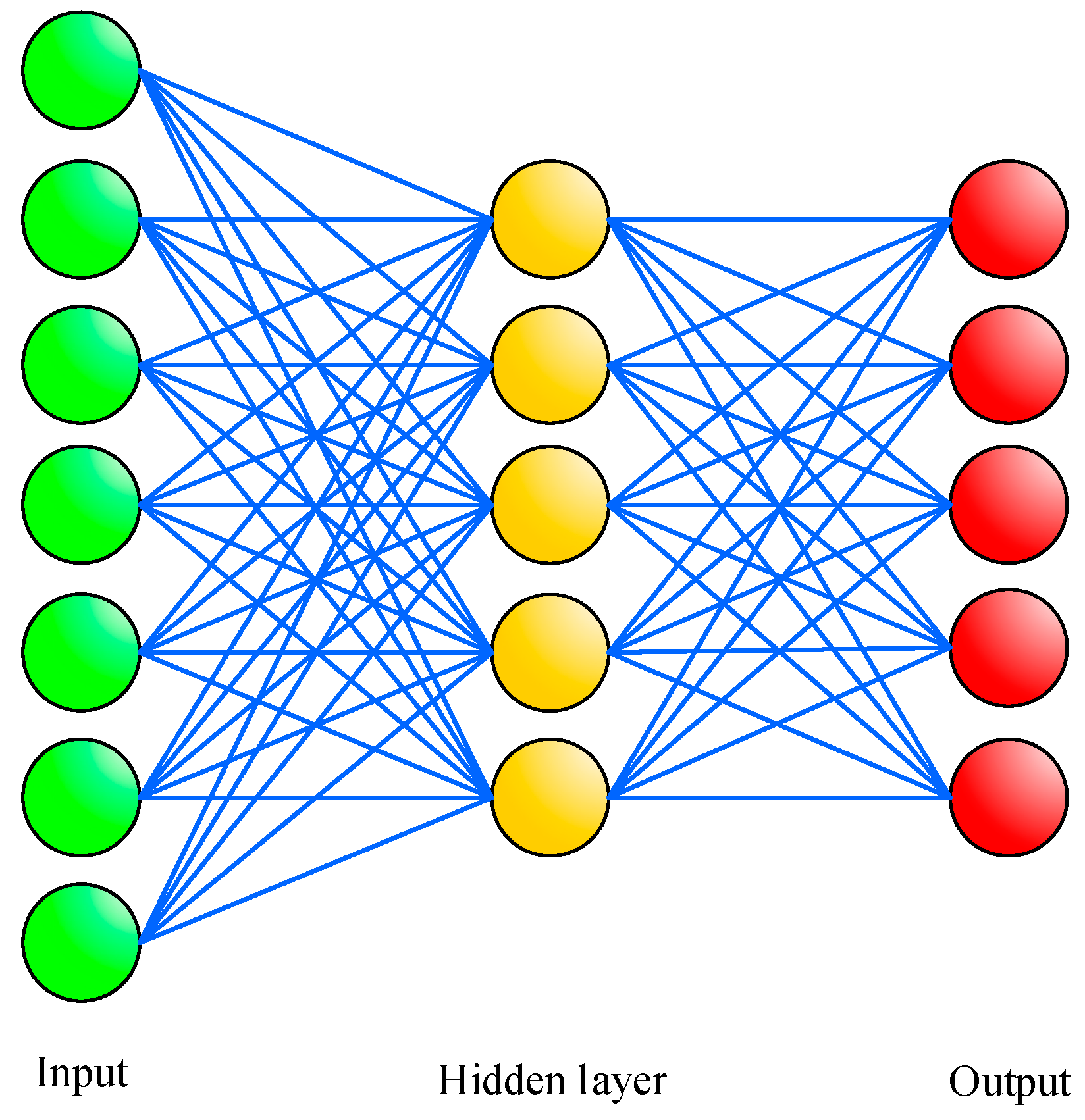
The basic computation unit in a neural network is a neuron, commonly referred to as a “node” or “unit”. The node receives input from other nodes or receives input from an external source and calculates the output. Each input is supplemented with “weight” (w), which depends on the relative importance of other inputs. Feedfoward neural network is the first invented and simplest artificial neural network. It contains multiple neurons (nodes) arranged in multiple layers. Nodes in adjacent layers have connections or edges. All connections are equipped with weights. In the definition of MLP, there is at least one hidden layer (excluding one input layer and one output layer). The architecture of the fully connected neural network is as illustrated in Figure 4. The leftmost green circle represents the hidden layer, the middle yellow circle corresponds to the hidden layer, the rightmost red circle serves as output and the blue line represents weight. In the MLP architecture, each layer is fully connected. The MLP uses backpropagation to adjust the weight value during each training session. Following the MLP training, the calculation result can be output through layer-by-layer transfer.
3.2. Convolution Neural Network
Although the performance of MLP seems efficient in all aspects, CNN could present an improved performance for feature extraction capabilities. CNN, which can perform feature extraction automatically, can be applied to image recognition and natural language processing. It can also effectively reduce the load of neural network training due to the introduction of the convolution layer concept. CNN is also a cognitive method that mimics the human brain. As an example, if a human brain identifies an image, it may initially notice the distinctly colored points, lines and planes and then identify them into different shapes such as eyes, nose and mouth. This abstraction process is identical to the way that the CNN algorithm builds the model. The convolution layer shifts the comparison of points to comparison of sections, through analyzing characteristics block by block. Then, the integrated comparison results are gradually stacked and a better identification result can be obtained.
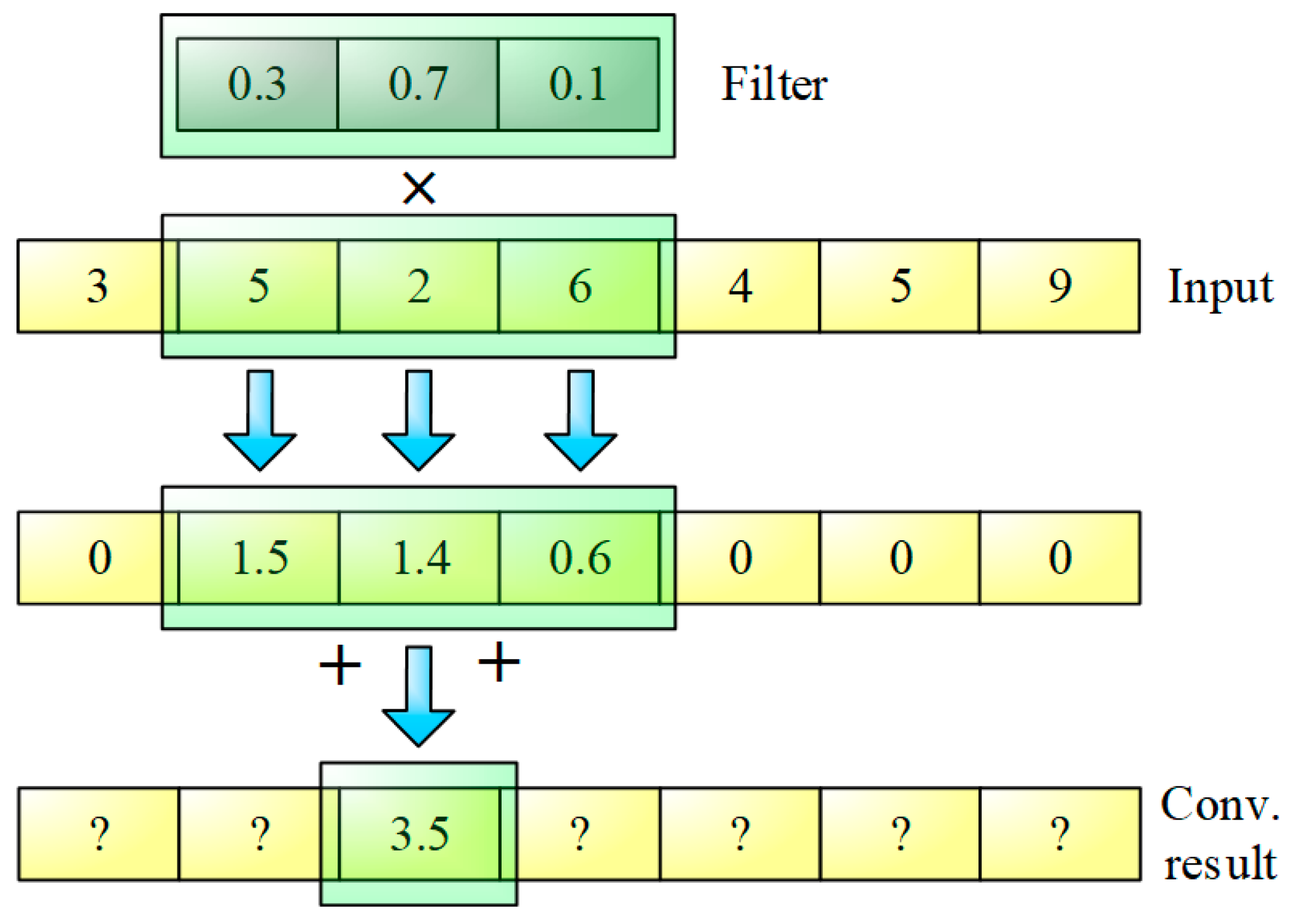
The 1D convolution process is as illustrated in Figure 5. The filter stands at the top of Figure 5. There are three weight values in the filter, hence in this example, its kernel size equals 3. The convolution process consists of the multiply of the corresponding sequence in the input by the weight value of the filter and adding the results. The filter will stride one by one in the input sequence to calculate the result. It is worth noting that the weight value on the filter is determined through backpropagation and is not determined manually. Unlike the MLP architecture, CNN uses a lower number of weights, which is one of the results that CNN can obtain faster convergence results.
3.3. The Proposed Model
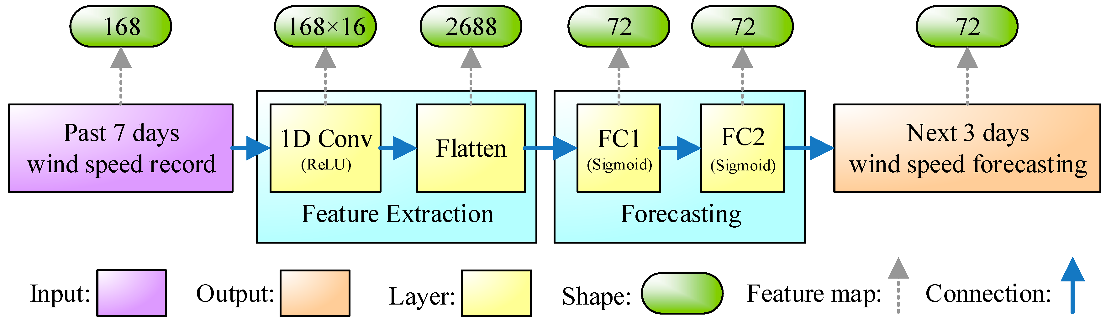
The WindNet model proposed in this paper is presented in Figure 6. WindNet incorporates CNN with fully connected architectures. The input of WindNet is the wind speed record for the past 7 days and the output is the wind speed estimation for the following 3 days. Since wind speed data is collected hourly, the data volume of the previous 7 days corresponds to 24 × 7 = 168 data sets, while the data volume of the following 3 days equals 24 × 3 = 72 sets. After collecting data from the previous 7 days, WindNet will perform 1D convolution. Here, authors used 16 filters to perform convolution, hence the feature map shape of 1D convolution equals 168 × 16. To facilitate the connection of the subsequent estimation framework, after the 1D convolution layer, the feature map was flattened, to turn the shape of its feature map back to one dimension. This is the feature extraction process. Subsequently, WindNet will import the extracted features into a 2-layer fully connected architecture. The number of fully connected neurons in both layers equals 72, which is identical to the output length. Finally, FC2 output corresponds to the wind speed forecast of the next 3 days.
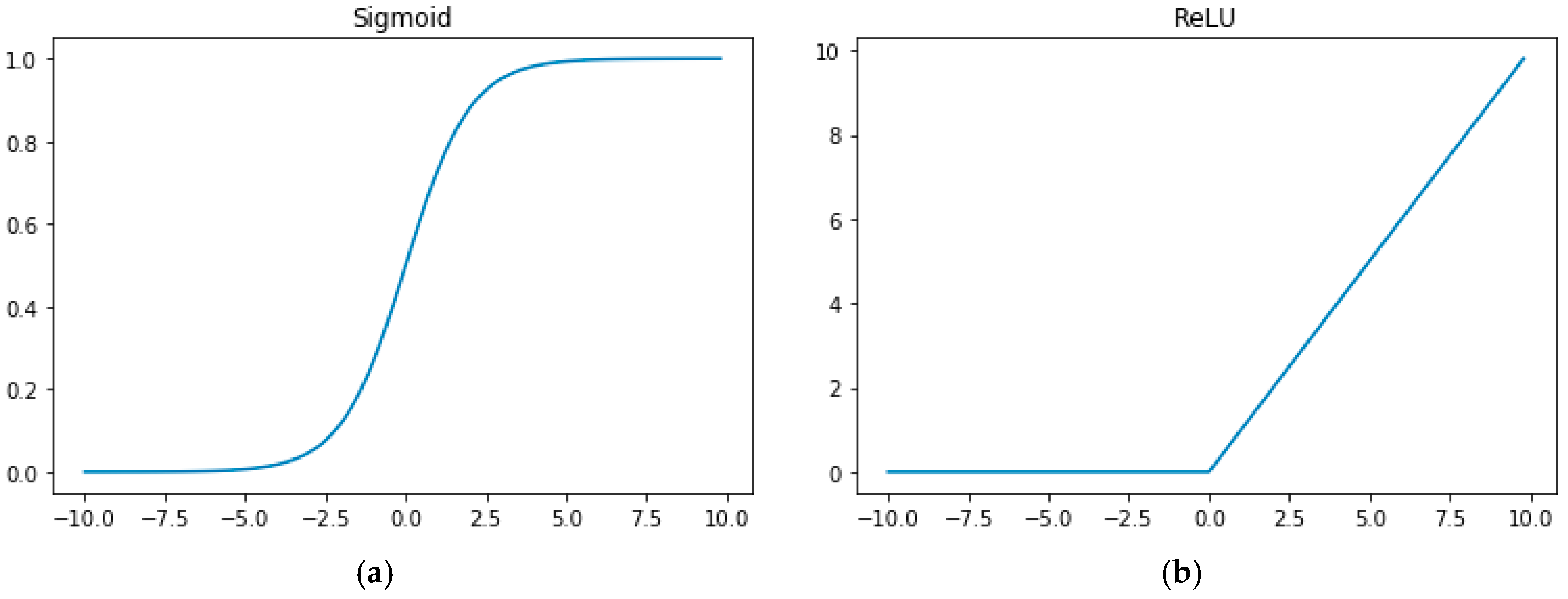
In WindNet, 2 activation functions were used: sigmoid and Rectified Linear Unit (ReLU). Related formulas are presented in Equations (1) and (2). In 1D convolution, the activation function used by WindNet is ReLU to minimize the problem of gradient vanishing. In the fully connected architecture in the latter layer, the sigmoid function was selected to limit the output value range to [0,1]. The sigmoid and ReLU diagrams are illustrated in Figure 7.
As it concerns the programming, the wind speed database will be read first to achieve data normalization. I In this process, the value range was limited to [0, 1]. Subsequently, these data will be categorized into training and testing data. The training data are used to train the model data, while the testing data are not used during the training process. Next, the Wind Net model is constructed and initialized. In each training period, to reduce data interdependency, all training data sequences are shuffled and training data are disassembled into several batches for training. In the WindNet architecture, the batch size equals 32, which means that there are 32 data in a batch. After training is completed, WindNet will use the testing data for performance evaluation. The program of the proposed WindNet is presented in Algorithm 1.
| Algorithm 1. The algorithm of the proposed WindNet. | |
| 1: | Loading the data |
| 2: | Data normalization |
| 3: | Partition the data into training data and testing data |
| 4: | Model initialization |
| 5: | For all epochs |
| 6: | Shuffle the order of the training data |
| 7: | Partition the training data into batches |
| 8: | For all batches |
| 9: | Train the model on batch |
| 10: | End |
| 11: | End |
| 12: | Performance evaluation |
| 13: | Terminate |
3.4. Stochastic Optimization
Deep learning often requires quantity of time and computing resources to train. Hence, this also corresponds to a major challenge for the development of deep learning algorithms. Although, multi-GPU parallel training can be used to accelerate the learning process of the model, the required computing resources are not reduced. An optimized algorithm, which requires fewer resources and allows the model to converge faster, can fundamentally accelerate the speed of the learning process and increase the effectiveness of the machine. To improve the training performance of the deep learning model, in current paper the adaptive moment estimation (Adam) optimizer was applied [32], which corresponds to a stochastic optimization algorithm, to adjust parameters. The Adam optimization algorithm is an extension of stochastic gradient descent (SGD), which is recently widely used in deep learning applications, especially for tasks such as computer visual and natural language processing. Adam is an optimization algorithm that can replace traditional SGD processes. It can iteratively update the weights of neural networks based on training data. The main formulas are presented in Equations (3)–(8).
α represents the step size, while β1 and β2 stand for the exponential decay rates. f(θ) is the stochastic objective function, θ0 equals the initial parameter vector, mt is 1st moment vector, vt corresponds to the 2nd moment vector, and are bias-corrected moment estimates, represents element wise square gt⊙gt. Kingma et al. [32], mentioned that effective initial settings are α = 0.001, β1 = 0.9, β2 = 0.999, ε = 10−8.
Adam is a very popular algorithm in deep learning since it can quickly achieve excellent results. Experimental results prove that the Adam algorithm has excellent performance during actual practice [32] and has great advantages compared to other kinds of random optimization algorithms. The detailed operation process of Adam is presented in Algorithm 2. Initially, after confirming parameters α, β1, β2 and stochastic objective function f(θ), the following parameters should be initialized: parameter vector θ, 1st moment vector mt, 2nd moment vector vt and timestep t. Then, as long as parameter θt does not converge, each part of the loop is iteratively updated. We also add 1 to timestep t, renew the stochastic objective function to the gradient requested by parameter θt at the timestep, update the biased first moment estimate mt, update biased second raw moment estimate vt, then calculate bias-corrected first moment estimate and bias-corrected second raw moment estimate , then update the model parameter θt with the above calculated value.
| Algorithm 2. The algorithm of Adam [32]. | |
| 1: | Require: α: Step size |
| 2: | Require: β1, β2 ∈ [0, 1): Exponential decay rates for the moment estimates |
| 3: | Require: f(θ): Stochastic objective function with parameters θ |
| 4: | Require: θ0: Initial parameter vector |
| 5: | m0 ← 0 (Initialize 1st moment vector) |
| 6: | v0 ← 0 (Initialize 2nd moment vector) |
| 7: | t ← 0 (Initialize timestep) |
| 8: | whileθt not converged do |
| 9: | t ← t + 1 |
| 10: | Get gradients with respect to stochastic objective at timestep t |
| 11: | Update biased first moment estimate |
| 12: | Update biased second raw moment estimate |
| 13: | Compute bias-corrected first moment estimate |
| 14: | Compute bias-corrected second raw moment estimate |
| 15: | Update θt parameters |
| 16: | end while |
| 17: | Returnθt (Resulting parameters) |
| 18: | Terminate |
4. Experimental Results
This chapter is divided into 2 parts: data description and experimental results. To demonstrate completely the performance of WindNet proposed in this paper, this chapter will also include comparisons of very popular and commonly used machine learning algorithms, such as support vector machine (SVM) [33,34,35,36,37,38], random forest (RF) [39,40,41,42,43,44], decision tree (DT) [45,46,47,48,49,50] and MLP.
4.1. Data Descriptions
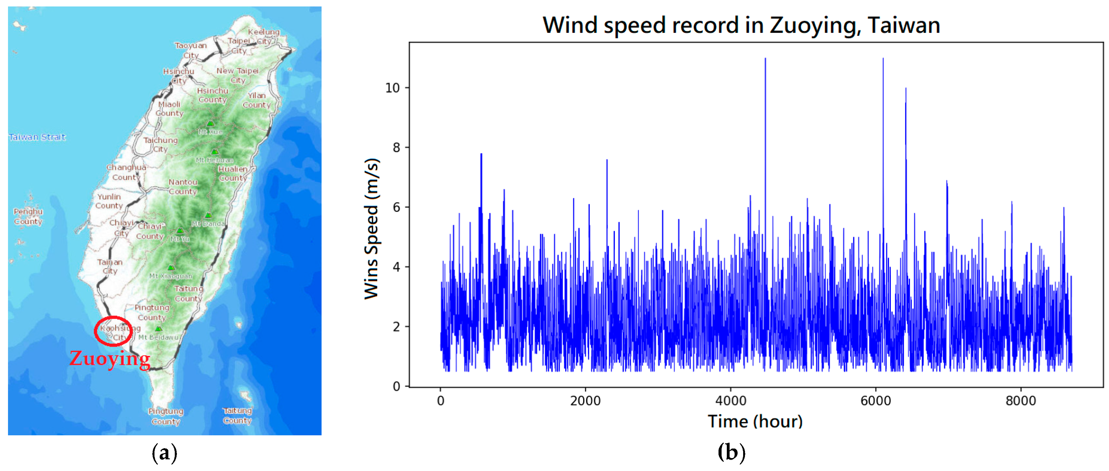
This experiment used the wind speed record reported by Zuoying, Taiwan in 2016 for performance analysis. The wind speed profile is illustrated in Figure 8b. The length of the collected data is one year, and it includes 8784 records. We have already tried other collected data in our previous research. However, according to that, the wind speed of Zuoying mostly falls at a range of 1.5 m/s to 4 m/s. There are still many cases where the wind speed is higher than 5 m/s or even exceeds 10 m/s. Based on Figure 8a, it can be derived that Zuoying is located in the offshore area. Thus the wind speed of Zuoying is not very stable and there are often sudden peaks. Therefore, it was difficult to predict wind speed. This is also the reason we choose this dataset for the experiments in this paper. In this experiment, the wind speed information of the past 7 days were used to predict the wind speed of the following 3 days. Authors estimated that through this information, the machine learning model will undergo supervised learning and analysis to achieve accurate predictions.
4.2. Experiment Results
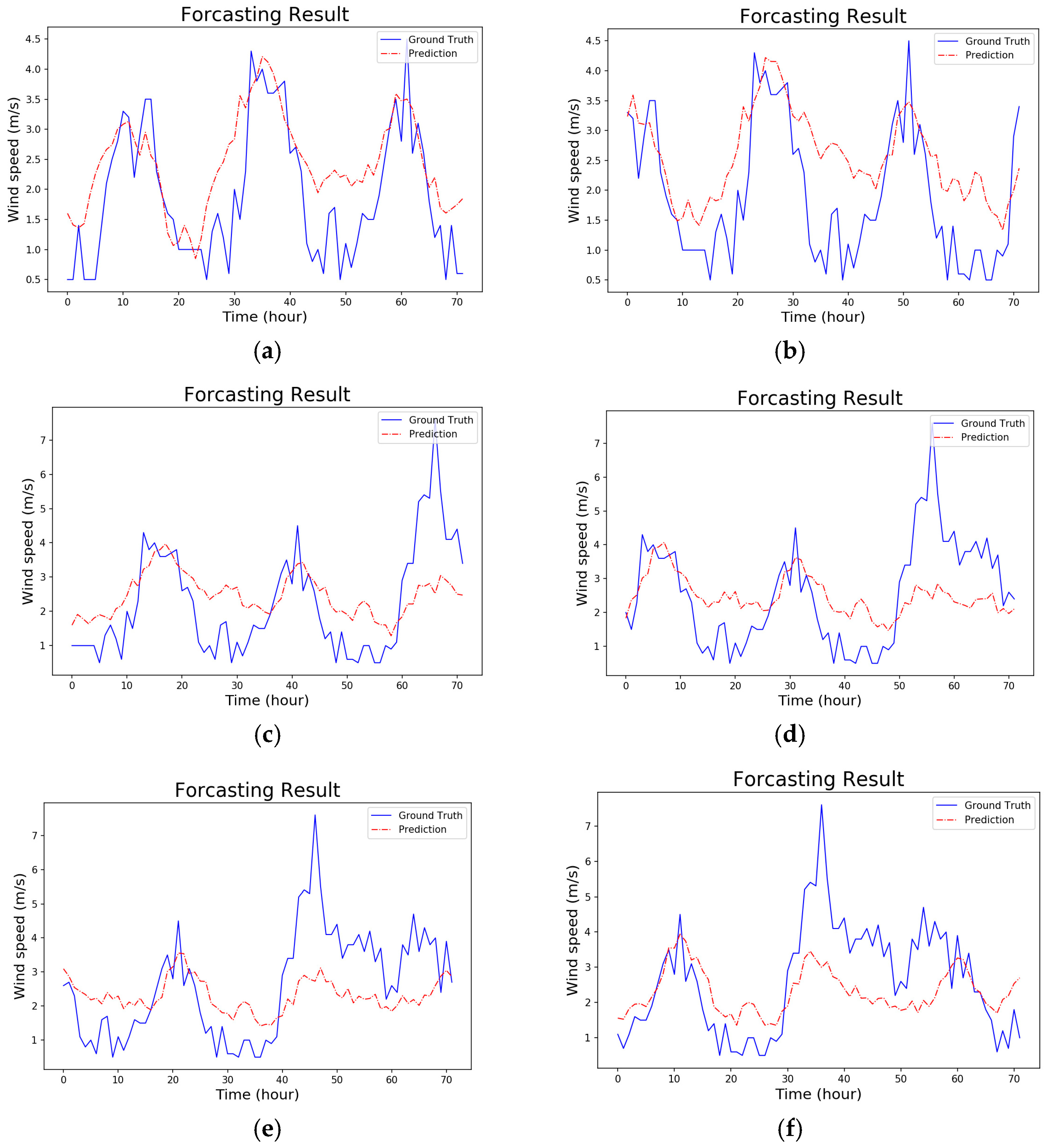
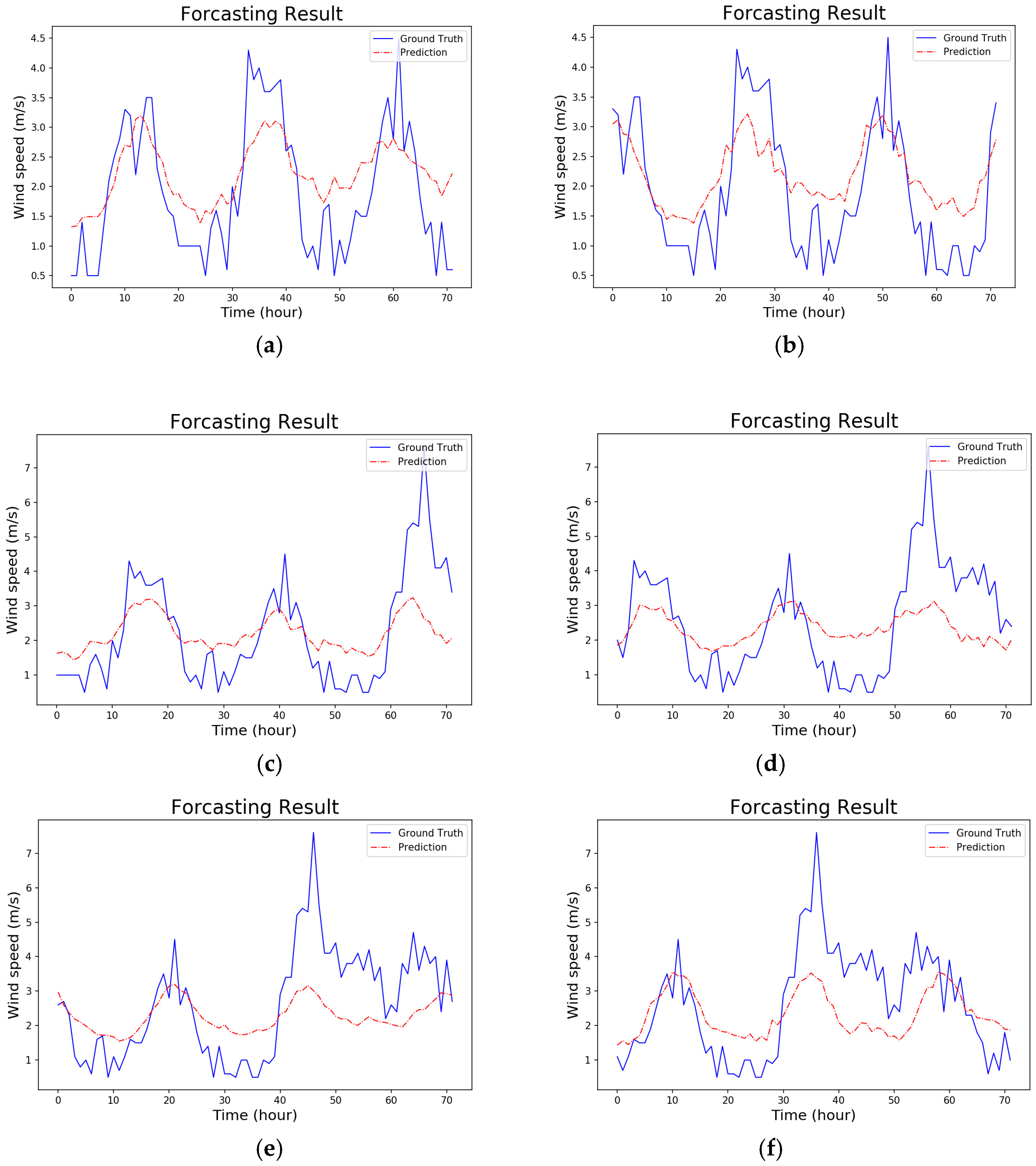
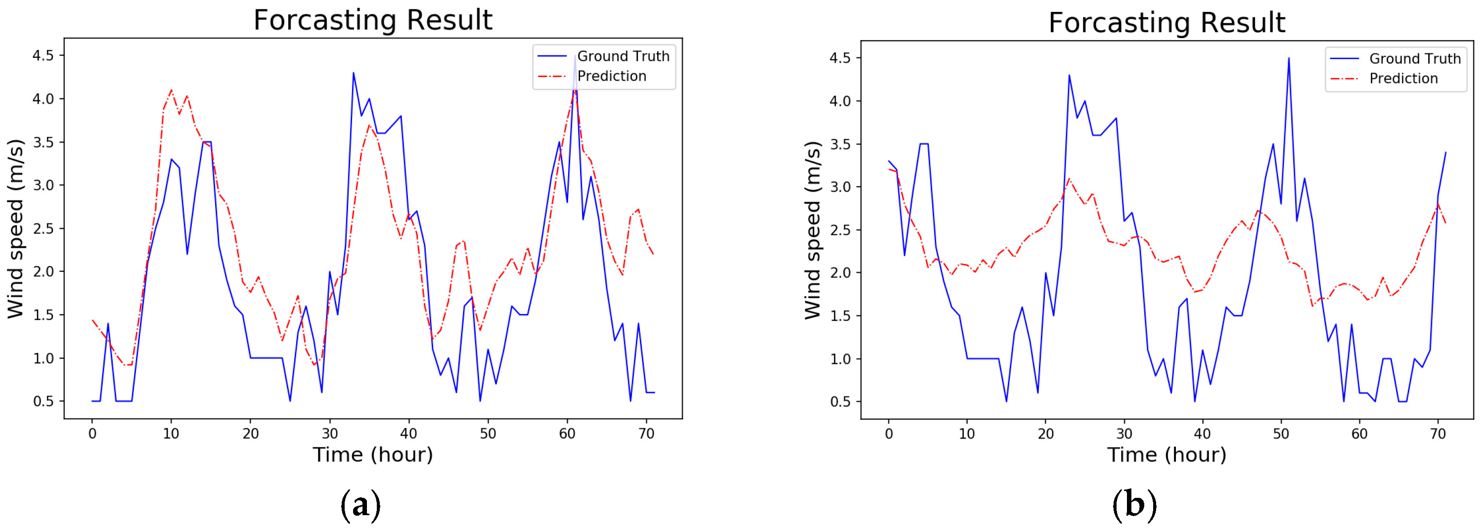
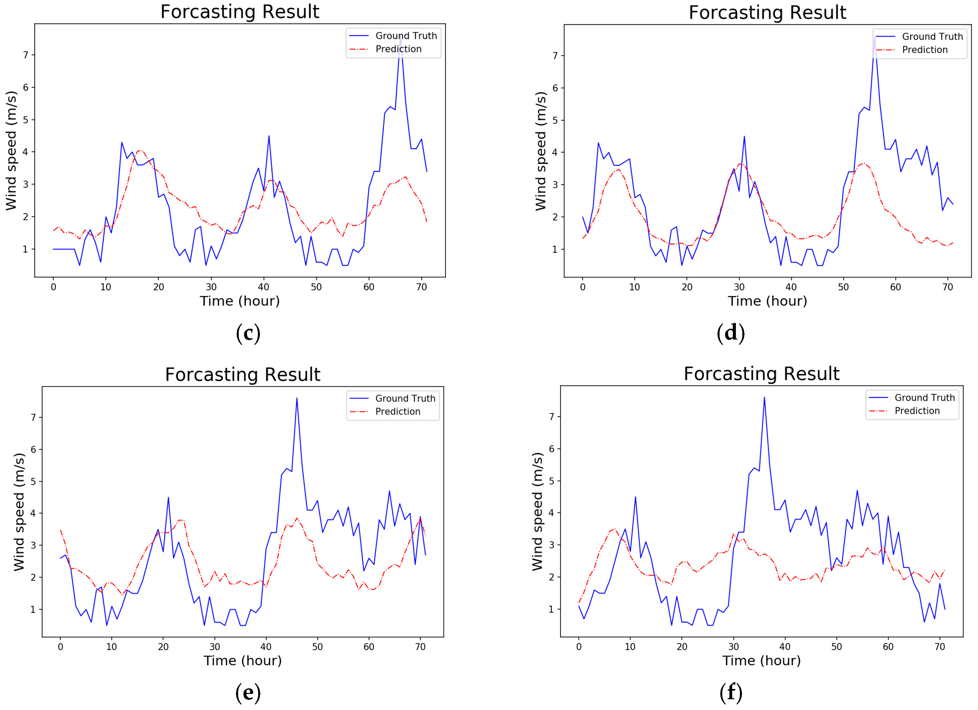
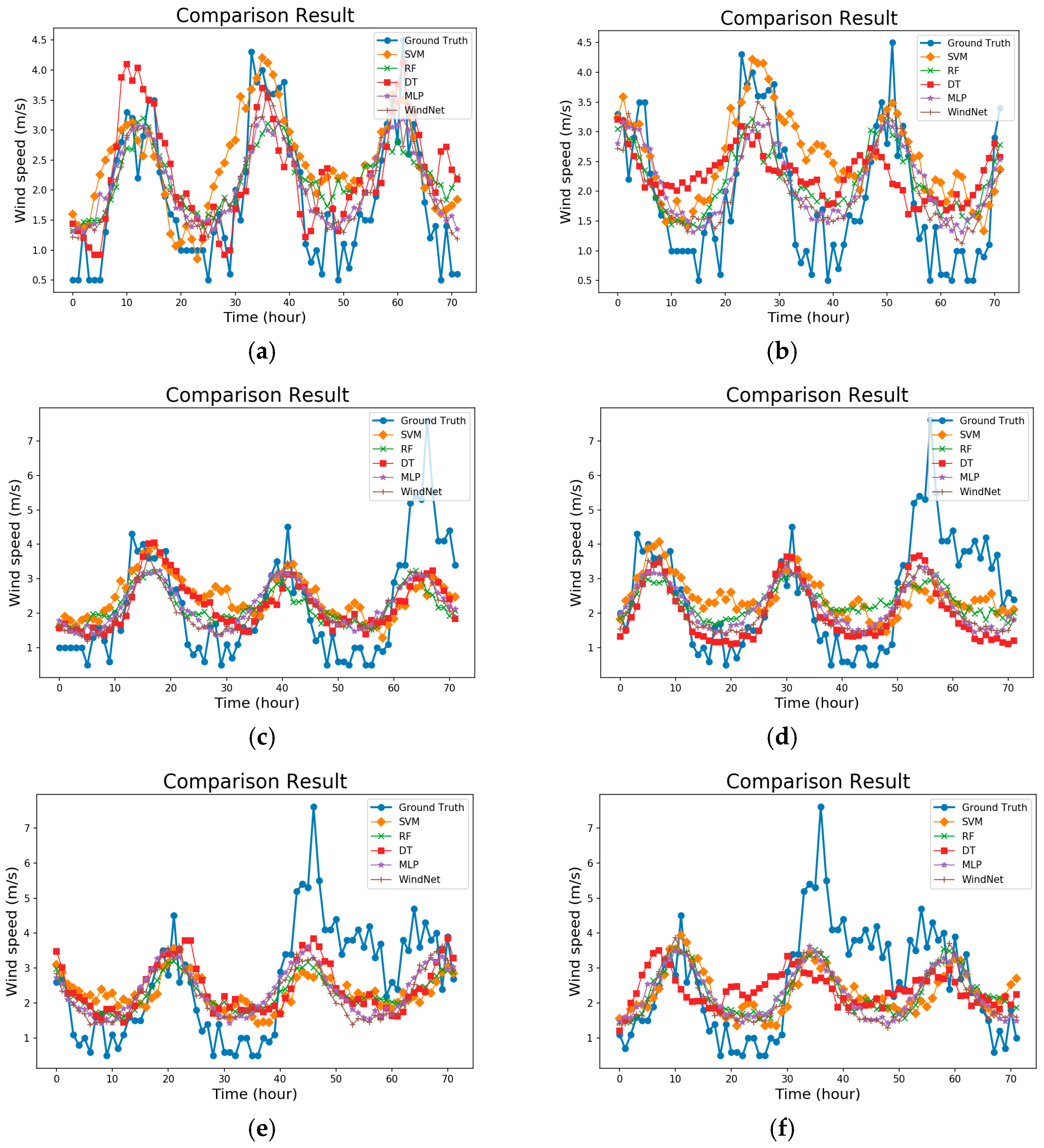
In this experiment, the mean absolute error (MAE) and root-mean-square error (RMSE) were applied as evaluation indicators (the formulas are shown in Equations (9) and (10) respectively). The test results of various algorithms are illustrated in Figure 9, Figure 10, Figure 11, Figure 12 and Figure 13. Figure 14 presents a comprehensive comparison of the entire algorithms. In actual situations, the forecasting model can only use past experience to predict future wind speed. When the model training is completed, the data used for real forecasting will be information that the trained model has never encountered before. Therefore, to meet real situations, in this experiment, testing data did not participated in the model training process and the experimental results obtained in this experiment were also based on testing data for performance evaluation. We can derive from Figure 14 that each algorithm can slightly capture the trends of future wind speeds, but the prediction results of SVM and DT are relatively unstable. Compared to that of SVM and DT, the performance of RF, MLP and WindNet present increased stability. In particular, the wind speed information forecasted y WindNet is similar to the real conditions (as presented by the blue line). This confirms that WindNet is very effective and accurate in wind speed forecasting:
To perform an increased reliability test, authors extracted 11 segments from the dataset, each containing 2 months of training data and one month of testing data, and conducted model training and testing on the data of these 11 segments. The test results are presented in Table 1 (MAE) and Table 2 (RMSE). In MAE ranking from the lowest to the highest corresponds to: WindNet (0.800227), RF (0.831981), MLP (0.833486), DT (0.955564), SVM (0.967744). In RMSE ranking from the lowest to the highest corresponds to: WindNet (0.999978), MLP (1.022898), RF (1.030018), SVM (1.198929), DT (1.203666). According to the experimental results, authors concluded that compared with other algorithms, SVM and DT performed poorly, while the MAE and RMSE values of SVM and DT are identical. If MAE is used as a benchmark, DT outperforms SVM, but in RMSE, SVM outperforms DT. An identical situation also occurs for both the MLP and RF algorithms. If the comparison is based on MAE, RF performs better than MLP, but in RMSE, MLP outperforms RF. Although the performance of RF and MLP is efficient, in terms of MAE or RMSE measurements, the leading performance overall is still the WindNet model proposed in this article.
5. Discussion
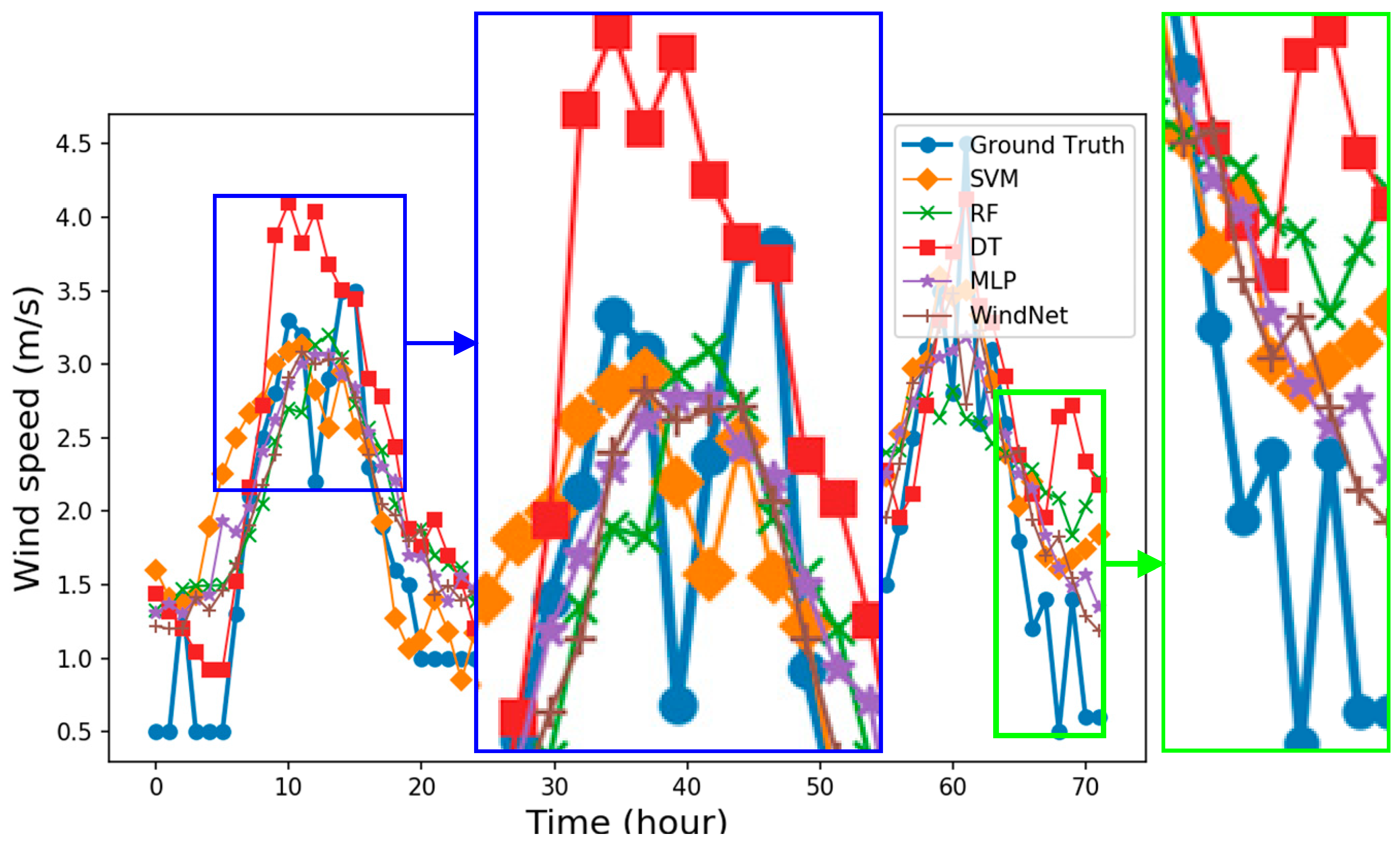
The choosing of the parameters is also a very important issue during the training process. By the correct parameter setting of WindNet, as shown in Table 3, the performance of the proposed WindNet can be significantly demonstrated. Figure 15 presents the detailed comparison result of each model. The thick blue line corresponds to the actual data and the lines of other colors are the prediction results of various algorithms. The blue box in Figure 15 indicates that the prediction result of DT almost does not coincide with the actual data, while the trend forecasted by SVM also does not coincide with that of the actual data. Among all algorithms, RF, MLP and WindNet still perform better. The green box in Figure 15 demonstrates that when the wind speed is about to decrease, many algorithms struggle to grasp the trend, DT and SVM in particular, miscalculated the trend. Even RM cannot accurately forecast data and presents a relatively disordered situation. This points out that there is still a certain degree of difficulty to the forecasting of wind speed. However, even if many algorithms cannot accurately predict data, MLP and WindNet can still supply stable forecast results. Overall, the performances of RF and MLP are stable and accurate. Nevertheless, WindNet produced the most efficient results. Therefore, the ability of WindNet for wind speed forecasting has been proven in this experiment.
6. Conclusions
In the field of renewable energy research, the quality of the energy management system corresponds to a crucial aspect in the power dispatching process. Additionally, wind speed forecasting is a significant parameter. To solve the problem of wind speed forecasting and improve its prediction capacity, this paper proposes a CNN architecture wind speed forecasting system called WindNet. WindNet can predict the wind speed for the following 3 days based on wind speed data from the previous 7 days. To verify absolutely the effectiveness of the WindNet architecture proposed in this paper, we use RMSE and MAE indicators to estimate the performance in the experiment and compare it to that of multiple other machine learning algorithms. In this paper, the forecasting performance of the proposed algorithm was compared to that of four other artificial intelligence algorithms commonly used in wind speed forecasting, such as SVM, RF, DT, and MLP. In the experiment, authors used wind speed data from Zuoying, Taiwan for model training and performance estimation. The experimental data in this paper were categorized into training and testing data. Training data were used for the training of the model, while testing data that has never been used in the training process performed the MAE and RMSE calculations to estimate the performance. The MAE and RMSE values of the proposed algorithm are 0.800227 and 0.999978, respectively. Experimental results indicate that WindNet achieves the most efficient results in both RMSE and MAE. During this experiment, the feasibility and effectiveness of proposed WindNet model have been entirely verified.
Author Contributions
C.-J.H. designed this study and collected the dataset. P.-H.K. wrote the program and designed the model. C.-J.H. and P.-H.K. contributed in drafted and revised the manuscript.
Funding
This work was performed under auspices of the Jiangxi University of Science and Technology, People’s Republic of China, under Grants jxxjbs18019.
Conflicts of Interest
The authors declare no conflict of interest.
References
- Soman, S.S.; Zareipour, H.; Malik, O.; Mandal, P. A review of wind power and wind speed forecasting methods with different time horizons. N. Am. Power Symp. 2010. [Google Scholar] [CrossRef]
- Georgilakis, P.S. Technical challenges associated with the integration of wind power into power systems. Renew. Sustain. Energy Rev. 2008, 12, 852–863. [Google Scholar] [CrossRef] [Green Version]
- Foley, A.M.; Leahy, P.G.; Marvuglia, A.; McKeogh, E.J. Current methods and advances in forecasting of wind power generation. Renew. Energy 2012, 37, 1–8. [Google Scholar] [CrossRef] [Green Version]
- Ponta, L.; Raberto, M.; Teglio, A.; Cincotti, S. An Agent-based Stock-flow Consistent Model of the Sustainable Transition in the Energy Sector. Ecol. Econ. 2018, 145, 274–300. [Google Scholar] [CrossRef] [Green Version]
- Matson, P. The Sustainability Transition. Available online: https://issues.org/matson/ (accessed on 29 September 2018).
- Tascikaraoglu, A.; Uzunoglu, M. A review of combined approaches for prediction of short-term wind speed and power. Renew. Sustain. Energy Rev. 2014, 34, 243–254. [Google Scholar] [CrossRef]
- Kuo, P.-H.; Huang, C.-J. An Electricity Price Forecasting Model by Hybrid Structured Deep Neural Networks. Sustainability 2018, 10, 1280. [Google Scholar] [CrossRef]
- Cincotti, S.; Gallo, G.; Ponta, L.; Raberto, M. Modeling and forecasting of electricity spot-prices: Computational intelligence vs classical econometrics. AI Commun. 2014, 27, 301–314. [Google Scholar] [CrossRef]
- De Filippo, A.; Lombardi, M.; Milano, M. User-Aware Electricity Price Optimization for the Competitive Market. Energies 2017, 10, 1378. [Google Scholar] [CrossRef]
- Jung, J.; Broadwater, R.P. Current status and future advances for wind speed and power forecasting. Renew. Sustain. Energy Rev. 2014, 31, 762–777. [Google Scholar] [CrossRef]
- Chang, T.P.; Liu, F.J.; Ko, H.H.; Huang, M.C. Oscillation characteristic study of wind speed, global solar radiation and air temperature using wavelet analysis. Appl. Energy 2017, 190, 650–657. [Google Scholar] [CrossRef]
- Pfeifer, S.; Schönfeldt, H.J. The response of saltation to wind speed fluctuations. Earth Surf. Process. Landf. 2012, 37, 1056–1064. [Google Scholar] [CrossRef]
- Chang, W.-Y. A Literature Review of Wind Forecasting Methods. J. Power Energy Eng. 2014, 2, 161–168. [Google Scholar] [CrossRef]
- Jiang, Y.; Song, Z.; Kusiak, A. Very short-term wind speed forecasting with Bayesian structural break model. Renew. Energy 2013, 50, 637–647. [Google Scholar] [CrossRef]
- Bouzgou, H. A fast and accurate model for forecasting wind speed and solar radiation time series based on extreme learning machines and principal components analysis. J. Renew. Sustain. Energy 2014, 6. [Google Scholar] [CrossRef]
- Wang, J.; Song, Y.; Liu, F.; Hou, R. Analysis and application of forecasting models in wind power integration: A review of multi-step-ahead wind speed forecasting models. Renew. Sustain. Energy Rev. 2016, 60, 960–981. [Google Scholar] [CrossRef]
- Ren, Y.; Suganthan, P.N.; Srikanth, N. Ensemble methods for wind and solar power forecasting—A state-of-the-art review. Renew. Sustain. Energy Rev. 2015, 50, 82–91. [Google Scholar] [CrossRef]
- Jiang, P.; Wang, Y.; Wang, J. Short-term wind speed forecasting using a hybrid model. Energy 2017, 119, 561–577. [Google Scholar] [CrossRef]
- Zhang, J.; Wei, Y.; Tan, Z.; Ke, W.; Tian, W. A Hybrid Method for Short-Term Wind Speed Forecasting. Sustainability 2017, 9, 596. [Google Scholar] [CrossRef]
- More, A.; Deo, M.C. Forecasting wind with neural networks. Mar. Struct. 2003, 16, 35–49. [Google Scholar] [CrossRef]
- Li, G.; Shi, J. On comparing three artificial neural networks for wind speed forecasting. Appl. Energy 2010, 87, 2313–2320. [Google Scholar] [CrossRef]
- Guo, Z.; Zhao, W.; Lu, H.; Wang, J. Multi-step forecasting for wind speed using a modified EMD-based artificial neural network model. Renew. Energy 2012, 37, 241–249. [Google Scholar] [CrossRef]
- Fathima, A.H.; Palanisamy, K. Energy Storage Systems for Energy Management of Renewables in Distributed Generation Systems. Energy Manag. Distrib. Gener. Syst. 2016. [Google Scholar] [CrossRef] [Green Version]
- El Moursi, M.S.; Al Hinai, A.; Ssekulima, E.B.; Anwar, M.B. Wind speed and solar irradiance forecasting techniques for enhanced renewable energy integration with the grid: A review. IET Renew. Power Gener. 2016, 10, 885–989. [Google Scholar] [CrossRef]
- White, B.W.; Rosenblatt, F. Principles of Neurodynamics: Perceptrons and the Theory of Brain Mechanisms. Am. J. Psychol. 1963, 76, 705. [Google Scholar] [CrossRef]
- Krizhevsky, A.; Sutskever, I.; Hinton, G.E. ImageNet Classification with Deep Convolutional Neural Networks. Adv. Neural Inf. Process. Syst. 2012, 1–9. [Google Scholar] [CrossRef]
- Qiu, Z.; Chen, J.; Zhao, Y.; Zhu, S.; He, Y.; Zhang, C. Variety Identification of Single Rice Seed Using Hyperspectral Imaging Combined with Convolutional Neural Network. Appl. Sci. 2018, 8, 212. [Google Scholar] [CrossRef]
- Nam, S.; Park, H.; Seo, C.; Choi, D. Forged Signature Distinction Using Convolutional Neural Network for Feature Extraction. Appl. Sci. 2018, 8, 153. [Google Scholar] [CrossRef]
- Li, C.; Zhou, H. Enhancing the Efficiency of Massive Online Learning by Integrating Intelligent Analysis into MOOCs with an Application to Education of Sustainability. Sustainability 2018, 10, 468. [Google Scholar] [CrossRef]
- An, Q.; Pan, Z.; You, H. Ship Detection in Gaofen-3 SAR Images Based on Sea Clutter Distribution Analysis and Deep Convolutional Neural Network. Sensors 2018, 18, 334. [Google Scholar] [CrossRef] [PubMed]
- Lopez-Martin, M.; Carro, B.; Sanchez-Esguevillas, A.; Lloret, J. Network Traffic Classifier with Convolutional and Recurrent Neural Networks for Internet of Things. IEEE Access 2017, 5, 18042–18050. [Google Scholar] [CrossRef]
- Kingma, D.P.; Ba, J. Adam: A Method for Stochastic Optimization. Comput. Sci. 2014, 1–13. [Google Scholar] [CrossRef]
- Suykens, J.A.K.; Vandewalle, J. Least squares support vector machine classifiers. Neural Process. Lett. 1999, 9, 293–300. [Google Scholar] [CrossRef]
- Niu, D.; Li, Y.; Dai, S.; Kang, H.; Xue, Z.; Jin, X.; Song, Y. Sustainability Evaluation of Power Grid Construction Projects Using Improved TOPSIS and Least Square Support Vector Machine with Modified Fly Optimization Algorithm. Sustainability 2018, 10, 231. [Google Scholar] [CrossRef]
- Das, M.; Akpinar, E. Investigation of Pear Drying Performance by Different Methods and Regression of Convective Heat Transfer Coefficient with Support Vector Machine. Appl. Sci. 2018, 8, 215. [Google Scholar] [CrossRef]
- Wang, S.; Hae, H.; Kim, J. Development of easily accessible electricity consumption model using open data and GA-SVR. Energies 2018, 11, 373. [Google Scholar] [CrossRef]
- Liu, J.P.; Li, C.L. The short-term power load forecasting based on sperm whale algorithm and wavelet least square support vector machine with DWT-IR for feature selection. Sustainability 2017, 9, 1188. [Google Scholar] [CrossRef]
- Wang, J.; Niu, T.; Wang, R. Research and application of an air quality early warning system based on a modified least squares support vector machine and a cloud model. Int. J. Environ. Res. Public Health 2017, 14, 249. [Google Scholar] [CrossRef] [PubMed]
- Liaw, A.; Wiener, M. Classification and Regression by randomForest. R News 2002, 2, 18–22. [Google Scholar] [CrossRef]
- Ma, J.; Qiao, Y.; Hu, G.; Huang, Y.; Sangaiah, A.K.; Zhang, C.; Wang, Y.; Zhang, R. De-Anonymizing Social Networks with Random Forest Classifier. IEEE Access 2018, 6, 10139–10150. [Google Scholar] [CrossRef]
- Huang, N.; Lu, G.; Xu, D. A permutation importance-based feature selection method for short-term electricity load forecasting using random forest. Energies 2016, 9, 767. [Google Scholar] [CrossRef]
- Hassan, M.; Southworth, J. Analyzing Land Cover Change and Urban Growth Trajectories of the Mega-Urban Region of Dhaka Using Remotely Sensed Data and an Ensemble Classifier. Sustainability 2017, 10, 10. [Google Scholar] [CrossRef]
- Zhu, M.; Xia, J.; Jin, X.; Yan, M.; Cai, G.; Yan, J.; Ning, G. Class Weights Random Forest Algorithm for Processing Class Imbalanced Medical Data. IEEE Access 2018, 6, 4641–4652. [Google Scholar] [CrossRef]
- Quintana, D.; Sáez, Y.; Isasi, P. Random Forest Prediction of IPO Underpricing. Appl. Sci. 2017, 7, 636. [Google Scholar] [CrossRef]
- Safavian, S.R.; Landgrebe, D. A Survey of Decision Tree Classifier Methodology. IEEE Trans. Syst. Man Cybern. 1991, 21, 660–674. [Google Scholar] [CrossRef]
- Rau, C.-S.; Wu, S.-C.; Chien, P.-C.; Kuo, P.-J.; Chen, Y.-C.; Hsieh, H.-Y.; Hsieh, C.-H.; Liu, H.-T. Identification of Pancreatic Injury in Patients with Elevated Amylase or Lipase Level Using a Decision Tree Classifier: A Cross-Sectional Retrospective Analysis in a Level I Trauma Center. Int. J. Environ. Res. Public Health 2018, 15, 277. [Google Scholar] [CrossRef] [PubMed]
- Huang, N.; Peng, H.; Cai, G.; Chen, J. Power quality disturbances feature selection and recognition using optimal multi-resolution fast S-transform and CART algorithm. Energies 2016, 9, 927. [Google Scholar] [CrossRef]
- Rosli, N.; Rahman, M.; Balakrishnan, M.; Komeda, T.; Mazlan, S.; Zamzuri, H. Improved Gender Recognition during Stepping Activity for Rehab Application Using the Combinatorial Fusion Approach of EMG and HRV. Appl. Sci. 2017, 7, 348. [Google Scholar] [CrossRef]
- Alani, A.Y.; Osunmakinde, I.O. Short-term multiple forecasting of electric energy loads for sustainable demand planning in smart grids for smart homes. Sustainability 2017, 9, 1972. [Google Scholar] [CrossRef]
- Rau, C.-S.; Wu, S.-C.; Chien, P.-C.; Kuo, P.-J.; Chen, Y.-C.; Hsieh, H.-Y.; Hsieh, C.-H. Prediction of Mortality in Patients with Isolated Traumatic Subarachnoid Hemorrhage Using a Decision Tree Classifier: A Retrospective Analysis Based on a Trauma Registry System. Int. J. Environ. Res. Public Health 2017, 14, 1420. [Google Scholar] [CrossRef] [PubMed]
Figure 1.
Renewable energy management system architecture [23].
Figure 1.
Renewable energy management system architecture [23].

Figure 2.
The classification of different forecast methods [24].
Figure 2.
The classification of different forecast methods [24].

Figure 3.
The classification of prediction methods [24].
Figure 3.
The classification of prediction methods [24].

Figure 4.
The architecture of the fully connected neural network.

Figure 5.
The 1D convolution process.

Figure 6.
The architecture of the proposed WindNet model.

Figure 7.
The activation functions (a) Sigmoid, (b) ReLU.

Figure 8.
The information of (a) the position and (b) wind speed record in Zuoying, Taiwan.

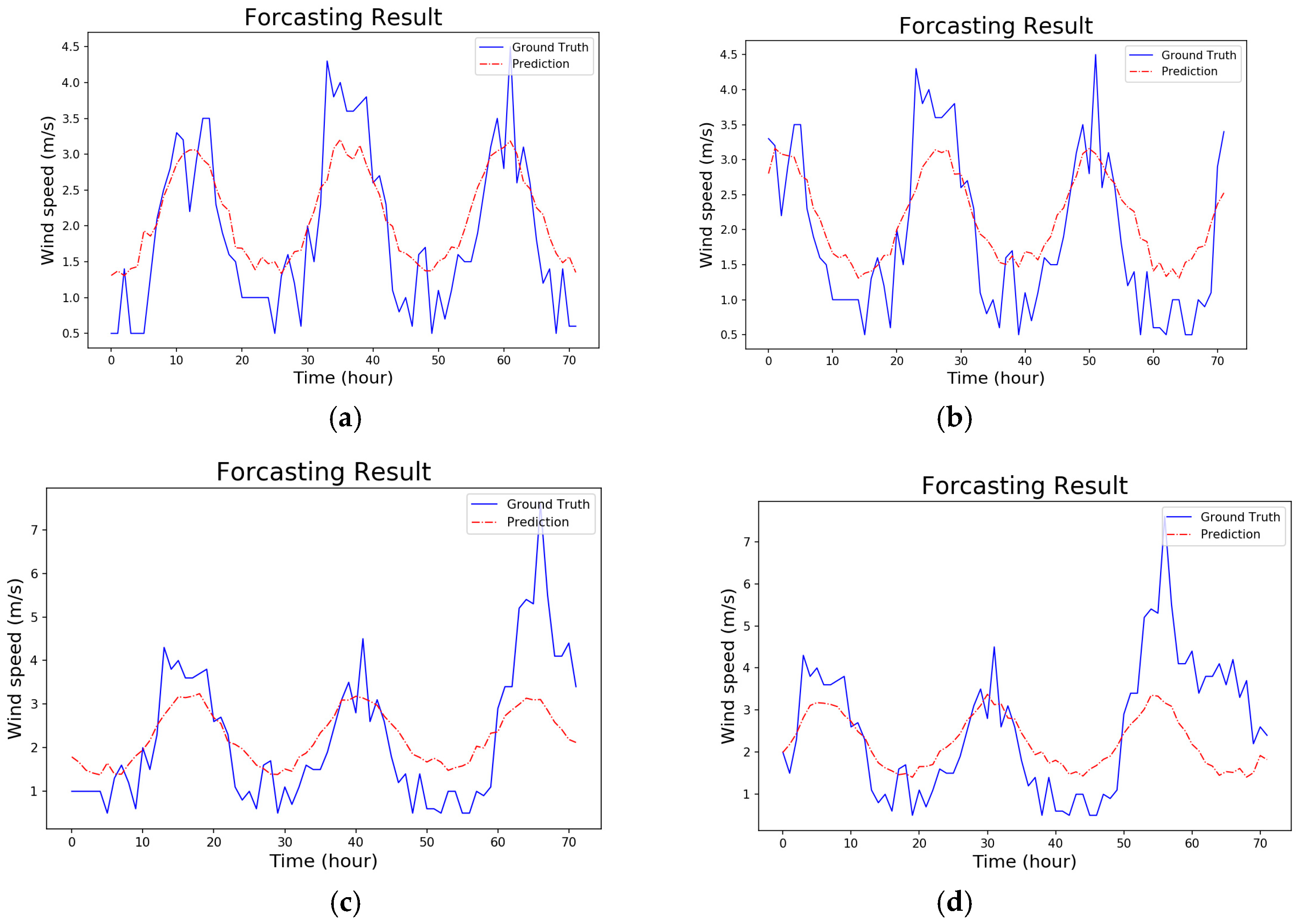
Figure 9.
The forecasting results of SVM: (a) Partial results A; (b) Partial results B; (c) Partial results C; (d) Partial results D; (e) Partial results E; (f) Partial results F.
Figure 9.
The forecasting results of SVM: (a) Partial results A; (b) Partial results B; (c) Partial results C; (d) Partial results D; (e) Partial results E; (f) Partial results F.

Figure 10.
The forecasting results of random forest: (a) Partial results A; (b) Partial results B; (c) Partial results C; (d) Partial results D; (e) Partial results E; (f) Partial results F.
Figure 10.
The forecasting results of random forest: (a) Partial results A; (b) Partial results B; (c) Partial results C; (d) Partial results D; (e) Partial results E; (f) Partial results F.

Figure 11.
The forecasting results of decision tree: (a) Partial results A; (b) Partial results B; (c) Partial results C; (d) Partial results D; (e) Partial results E; (f) Partial results F.
Figure 11.
The forecasting results of decision tree: (a) Partial results A; (b) Partial results B; (c) Partial results C; (d) Partial results D; (e) Partial results E; (f) Partial results F.


Figure 12.
The forecasting results of MLP: (a) Partial results A; (b) Partial results B; (c) Partial results C; (d) Partial results D; (e) Partial results E; (f) Partial results F.
Figure 12.
The forecasting results of MLP: (a) Partial results A; (b) Partial results B; (c) Partial results C; (d) Partial results D; (e) Partial results E; (f) Partial results F.


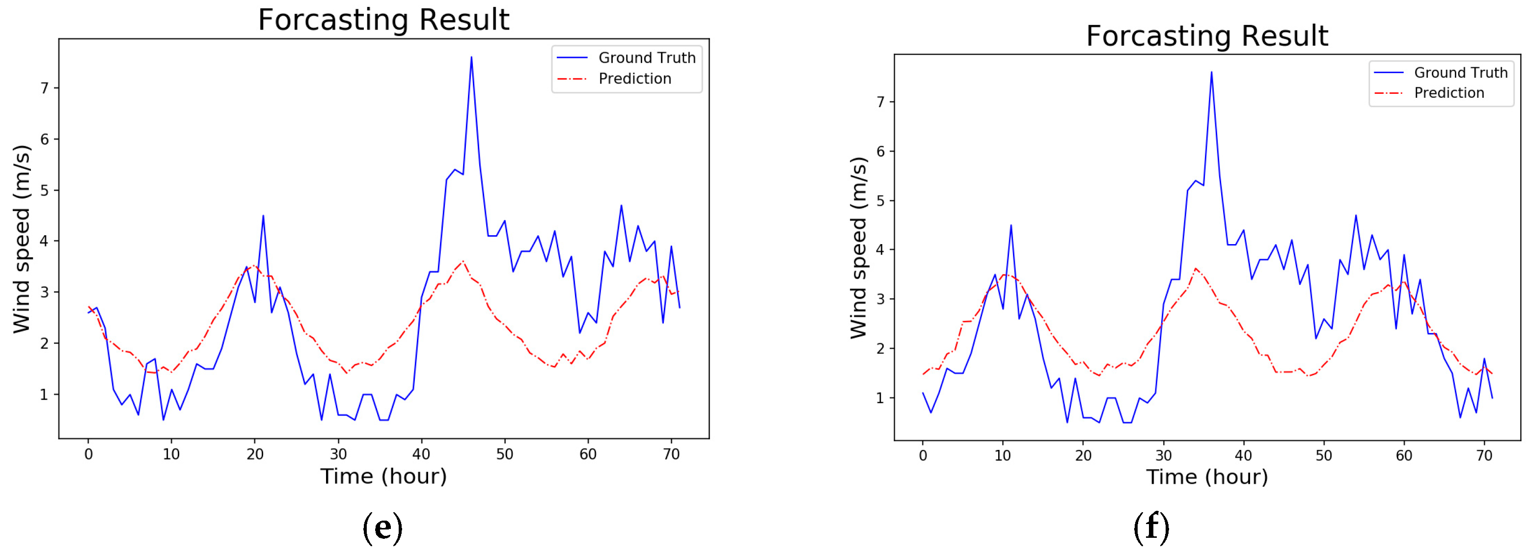
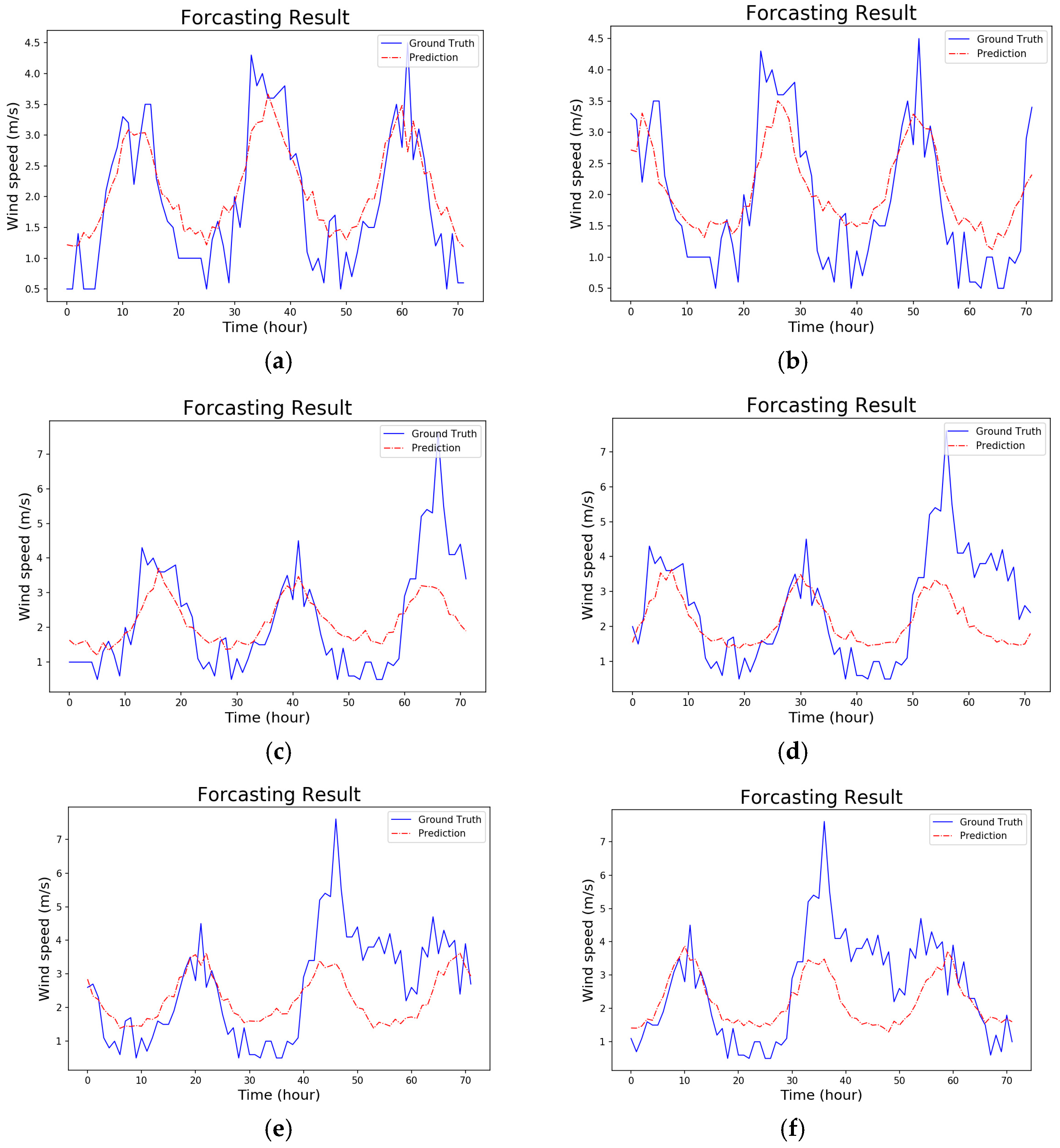
Figure 13.
The forecasting results of the proposed WindNet: (a) Partial results A; (b) Partial results B; (c) Partial results C; (d) Partial results D; (e) Partial results E; (f) Partial results F.
Figure 13.
The forecasting results of the proposed WindNet: (a) Partial results A; (b) Partial results B; (c) Partial results C; (d) Partial results D; (e) Partial results E; (f) Partial results F.

Figure 14.
The comparisons of all the forecasting results: (a) Partial results A; (b) Partial results B; (c) Partial results C; (d) Partial results D; (e) Partial results E; (f) Partial results F.
Figure 14.
The comparisons of all the forecasting results: (a) Partial results A; (b) Partial results B; (c) Partial results C; (d) Partial results D; (e) Partial results E; (f) Partial results F.

Figure 15.
The comparisons details of forecasting results.


Table 1.
The experimental results in terms of mean absolute error (MAE).
| Test | SVM | RF | DT | MLP | WindNet |
|---|---|---|---|---|---|
| #1 | 1.009532 | 1.010812 | 1.067496 | 0.951965 | 0.906002 |
| #2 | 0.804696 | 0.788575 | 0.91271 | 0.749479 | 0.726946 |
| #3 | 0.995466 | 0.876718 | 1.059931 | 0.883512 | 0.919904 |
| #4 | 0.824131 | 0.755548 | 0.839346 | 0.725489 | 0.735706 |
| #5 | 0.991768 | 0.987 | 1.10225 | 1.00744 | 0.956887 |
| #6 | 0.837221 | 0.769972 | 0.841412 | 0.845219 | 0.743931 |
| #7 | 1.004376 | 0.869387 | 1.009339 | 0.877877 | 0.867812 |
| #8 | 1.009328 | 0.825857 | 0.947832 | 0.832765 | 0.769551 |
| #9 | 1.154096 | 0.762744 | 0.89834 | 0.800525 | 0.744625 |
| #10 | 0.891498 | 0.694962 | 0.833799 | 0.742297 | 0.644439 |
| #11 | 1.123073 | 0.81022 | 0.998746 | 0.751773 | 0.786698 |
| Average | 0.967744 | 0.831981 | 0.955564 | 0.833486 | 0.800227 |
Table 2.
The experimental results in terms of root mean square error (RMSE).
| Test | SVM | RF | DT | MLP | WindNet |
|---|---|---|---|---|---|
| #1 | 1.212762 | 1.193097 | 1.280351 | 1.120047 | 1.084771 |
| #2 | 0.983817 | 0.965371 | 1.128812 | 0.915917 | 0.910913 |
| #3 | 1.227721 | 1.066804 | 1.310973 | 1.07933 | 1.136954 |
| #4 | 1.016498 | 0.933692 | 1.048922 | 0.90495 | 0.923487 |
| #5 | 1.296918 | 1.28096 | 1.41884 | 1.307386 | 1.252339 |
| #6 | 1.051861 | 0.973836 | 1.068395 | 1.037206 | 0.944069 |
| #7 | 1.226936 | 1.064154 | 1.267554 | 1.045251 | 1.059601 |
| #8 | 1.276431 | 1.046167 | 1.2283 | 1.044998 | 0.985753 |
| #9 | 1.373366 | 0.938822 | 1.143816 | 0.971037 | 0.922233 |
| #10 | 1.104978 | 0.859121 | 1.065049 | 0.903742 | 0.811998 |
| #11 | 1.416933 | 1.008177 | 1.279316 | 0.922009 | 0.967638 |
| Average | 1.198929 | 1.030018 | 1.203666 | 1.022898 | 0.999978 |
Table 3.
The parameter setting of WindNet.
| Parameter | Setting |
|---|---|
| 1D convolution filter number | 16 |
| 1D convolution kernel size | 9 |
| 1D convolution activation function | Rectified Linear Unit (ReLU) |
| Dense layer activation function | Sigmoid |
| Optimizer | Adaptive Moment Estimation (Adam) |
| Learning rate | 0.0005 |
| Learning rate decay | 0 |
| Loss function | Mean Squared Error (MSE) |
© 2018 by the authors. Licensee MDPI, Basel, Switzerland. This article is an open access article distributed under the terms and conditions of the Creative Commons Attribution (CC BY) license (http://creativecommons.org/licenses/by/4.0/).
Share and Cite
MDPI and ACS Style
Huang, C.-J.; Kuo, P.-H. A Short-Term Wind Speed Forecasting Model by Using Artificial Neural Networks with Stochastic Optimization for Renewable Energy Systems. Energies 2018, 11, 2777. https://0-doi-org.brum.beds.ac.uk/10.3390/en11102777
AMA Style
Huang C-J, Kuo P-H. A Short-Term Wind Speed Forecasting Model by Using Artificial Neural Networks with Stochastic Optimization for Renewable Energy Systems. Energies. 2018; 11(10):2777. https://0-doi-org.brum.beds.ac.uk/10.3390/en11102777
Chicago/Turabian StyleHuang, Chiou-Jye, and Ping-Huan Kuo. 2018. "A Short-Term Wind Speed Forecasting Model by Using Artificial Neural Networks with Stochastic Optimization for Renewable Energy Systems" Energies 11, no. 10: 2777. https://0-doi-org.brum.beds.ac.uk/10.3390/en11102777
Note that from the first issue of 2016, this journal uses article numbers instead of page numbers. See further details here.