Influence of Policy, Air Quality, and Local Attitudes toward Renewable Energy on the Adoption of Woody Biomass Heating Systems


Abstract
:1. Introduction
1.1. Land Ownership and Policy Influence on Biomass Use
1.2. Effects of Historic and Current Air Pollution on Biomass Use
1.3. Effects of Local Attitudes and Community Acceptance on Renewable Energy
1.4. Purpose, Goals and Objectives
2. Methods
2.1. Data
2.1.1. Policy Variables
2.1.2. Emissions Variables
Particulate Matter
Acid Rain
Greenhouse Gases
2.1.3. Local Attitudes
2.1.4. Other Control Variables
2.2. Statistical Methods
2.3. Model Diagnostics
3. Results
3.1. Model 1
3.2. Model 2
4. Discussion
5. Conclusions
Author Contributions
Funding
Conflicts of Interest
Abbreviations
| BLM | USA Bureau of Land Management |
| BRDI | Biomass Research and Development Initiative |
| CAA | Clean Air Act |
| CHP | Combined heat and power |
| CO2e | Carbon dioxide equivalent |
| d.f. | Degrees of freedom |
| DGP | Data generating process |
| DOE | USA Department of Energy |
| EIA | USA Energy Information Administration |
| EPA | USA Environmental Protection Agency |
| FIA | Forest Inventory and Analysis of USFS |
| FIP | Federal implementation plan |
| FWS | USA Fish and Wildlife Service |
| GHG | Greenhouse gas |
| HDD | Heating degree day |
| IRR | Incidence rate ratio |
| ISO4 | Interim Standard Offer 4 |
| MW | Megawatt |
| NAAQS | National Ambient Air Quality Standards |
| NB | Negative binomial |
| NIMBY | “Not in my back yard”, opposition on the basis of acute local impacts, but not their general characteristics |
| NOAA | USA National Oceanic and Atmospheric Administration |
| NOx | Nitrogen oxides |
| NSPS | New Source Performance Standards |
| Obs. | Observations |
| OR | Odds ratio |
| PM | Particulate matter |
| PM10 | Particulate matter with a diameter greater than 2.5 μm but smaller than 10 μm |
| PM2.5 | Particulate matter 2.5 μm in diameter or smaller |
| REC | Renewable energy certificate |
| RPS | Renewable portfolio standard |
| SE | Standard error |
| SIP | State implementation plan |
| SO2 | Sulfur dioxide |
| Std. Dev. | Standard deviation |
| TSP | Total suspended particulate |
| USA | United States of America |
| USDA | United States Department of Agriculture |
| USFS | United States Forest Service |
| W2E | Wood2Energy, see [1] |
| ZI | Zero inflated |
| ZINB | Zero inflated negative binomial |
| ZIP | Zero inflated Poisson |
References
- W2E. Wood2Energy Database 2014, the University of Tennessee, Center for Renewable Carbon, U.S. Endowment for Forestry and Communities. Available online: http://www.wood2energy.org/ (accessed on 26 September 2018).
- Nicholls, D.L.; Monserud, R.A.; Dykstra, D.P. A Synthesis of Biomass Utilization for Bioenergy Production in the Western United States; Gen. Tech. Rep. PNW-GTR-753; U.S. Department of Agriculture, Forest Service, Pacific Northwest Research Station: Portland, OR, USA, 2008; 48p.
- Wood, S.R.; Rowley, P.N. A techno-economic analysis of small scale, biomass-fueled combined heat and power for community housing. Biomass Bioenergy 2011, 35, 3849–3858. [Google Scholar] [CrossRef] [Green Version]
- Young, J.D. Economic and Policy Factors Driving Adoption of Institutional Woody Biomass Heating Systems in the United States. Master’s Thesis, University of Montana, Missoula, MT, USA, 16 May 2015. [Google Scholar]
- Young, J.D.; Anderson, N.M.; Naughton, H.T.; Mullan, K. Economic and policy factors driving adoption of institutional woody biomass heating systems in the United States. Energy Econ. 2018, 69, 456–470. [Google Scholar] [CrossRef]
- Becker, D.R.; Moseley, C.; Lee, C. A supply chain analysis framework for assessing state-level forest biomass utilization policies in the United States. Biomass Bioenergy 2011, 35, 1429–1439. [Google Scholar] [CrossRef]
- Yoo, J.; Ready, R.C. Preference heterogeneity for renewable energy technology. Energy Econ. 2014, 42, 101–114. [Google Scholar] [CrossRef]
- Summit Ridge Investments. Eastern Hardwood Forest Region WOODY Biomass Energy Opportunity; Summit Ridge Investments: Granville, Vermont, USA, 2007; 98p. [Google Scholar]
- U.S. Energy Information Administration. Renewables Energy Annual for 2008; Energy Information Administration: Washington, DC, USA, 2009. Available online: https://www.eia.gov/renewable/annual/ (accessed on 26 September 2018).
- U.S. Energy Information Administration. Definitions of Energy-Use Sectors and Related Terms; Energy Information Administration: Washington, DC, USA, 2010. Available online: http://www.eia.doe.gov/neic/datadefinitions/sectors25B1.htm (accessed on 28 September 2018).
- Congressional Research Service (CRS). Federal Land Ownership: Overview and Data; Congressional Research Service: Washington, DC, USA, 2012; 24p, Available online: https://fas.org/sgp/crs/misc/R42346.pdf (accessed on 28 September 2018).
- U.S. Census Bureau. Statistical Abstract of the United States: 2012; United States Census Bureau: Washington, DC, USA, 2012; 1460p. Available online: https://www.census.gov/library/publications/2011/compendia/statab/131ed.html (accessed on 28 September 2018).
- Becker, D.R.; Larson, D.; Lowell, E.C. Financial Considerations of policy options to enhance biomass utilization for reducing wildfire hazards. For. Policy Econ. 2009, 11, 628–635. [Google Scholar] [CrossRef]
- Schoennagel, T.; Nelson, C.R.; Theobald, D.M.; Carnwath, G.C.; Chapman, T.B. Implementation of National Fire Plan treatments near the wildland–urban interface in the western United States. Proc. Natl. Acad. Sci. USA 2009, 106, 10706–10711. [Google Scholar] [CrossRef] [PubMed]
- U.S. Government Accountability Office. Natural Resources. Federal Agencies are Engaged in Various Utilization of Woody biomass, but Significant Obstacles to Its Use Remain, GAO-05-373; United States Government Accountability Office: Washington, DC, USA, 2005; 17p. Available online: https://www.gao.gov/products/GAO-05-741T (accessed on 28 September 2018).
- NFPORS. National Fire Plan Operations and Reporting System; U.S. Department of the Interior: Washington, DC, USA. Available online: https://usgs.nfpors.gov/NFPORS_training/help/help.html?Request=Location (accessed on 26 September 2018).
- Public Law No. 106-224, Title III, 114 Stat. 428. 2000. Available online: http://www.gpo.gov/fdsys/pkg/PLAW-106publ224/html/PLAW-106publ224.htm (accessed on 26 September 2018).
- Public Law No. 108-148, Title II, 117 Stat. 1901. 2003. Available online: http://www.fs.fed.us/spf/tribalrelations/documents/policy/statutes/PL_108-148_HFRA.pdf (accessed on 26 September 2018).
- Aguilar, F.X.; Saunders, A. Policy instruments promoting wood for energy uses: Evidence from the continental U.S. J. For. 2010, 108, 132–140. [Google Scholar]
- Dykstra, D.P.; Nicholls, D.L.; Monserud, R.A. Biomass Utilization for Bioenergy in the Western United States. For. Prod. J. 2008, 58, 6–16. [Google Scholar]
- Leefers, L. Wood-Based Electric Power Generation in Michigan: Wood Use and Policies. For. Prod. J. 2011, 61, 586–591. [Google Scholar] [CrossRef]
- Uski, O.J.; Happo, M.S.; Jalava, P.I.; Brunner, T.; Kelz, J.; Obernberger, I.; Jokiniemi, J.; Hirvonen, M.R. Acute systemic and lung inflammation in C57Bl/6J mice after intra-tracheal aspiration of particulate matter from small-scale biomass combustion appliances based on old and modern technologies. Inhal. Toxicol. 2012, 24, 952–965. [Google Scholar] [CrossRef] [PubMed]
- Van Loo, S.; Koppejan, J. The Handbook of Biomass Combustion and Co-Firing; Earthscan Publishing: Washington, DC, USA, 2008; 442p. [Google Scholar]
- Bowman, B.C.; Forsberg, A.B.; Jarvholm, B.G. Adverse health effects from ambient air pollution in relation to residential wood combustion in modern society. Scand. J. Work Environ. Health 2003, 29, 251–260. [Google Scholar] [CrossRef] [Green Version]
- Koenig, J.Q.; Jansen, K.; Mar, T.F.; Lumley, T.; Kaufman, J.; Trenga, C.A.; Sullivan, J.; Liu, L.J.; Shapiro, G.G.; Larson, T.V. Measurement of offline exhaled nitric oxide in a study of community exposure to air pollution. Environ. Health Perspect. 2003, 111, 1625–1629. [Google Scholar] [CrossRef] [PubMed]
- Lipsett, M.; Hurley, S.; Ostro, B. Air pollution and emergency room visits for asthma in Santa Clara County, California. Environ. Health Perspect. 1997, 105, 216–222. [Google Scholar] [CrossRef] [PubMed]
- Krajick, K. Long-term data show lingering effects from acid rain. Science 2001, 292, 195–196. [Google Scholar] [CrossRef] [PubMed]
- Lieb, A.M.; Darrouzet-Nardi, A.; Bowman, W.D. Nitrogen deposition decreases acid buffering capacity of alpine soils in the southern Rocky Mountains. Geoderma 2011, 164, 220–224. [Google Scholar] [CrossRef]
- Squalli, J. Renewable energy, coal as a baseload power source, and greenhouse gas emissions: Evidence from U.S. state-level data. Energy 2017, 127, 479–488. [Google Scholar] [CrossRef]
- Salzman, J.; Thompson, B.H. Environmental Law and Policy, 3rd ed.; Foundation Press: New York, NY, USA, 2010; pp. 87–112. [Google Scholar]
- Flatt, V.B.; Connolly, K.D. ‘Grandfathered’ Air Pollution Sources and Pollution Control: New Source Review under the Clean Air Act; A Center for Progressive Regulation White Paper; Center for Progressive Regulation: Washington, DC, USA, 2005; 13p. [Google Scholar]
- Villeneuve, J.; Palacios, J.H.; Savoie, P.; Godbout, S. A critical review of emissions standards and regulations regarding biomass combustion in small scale units (<3 MW). Bioresour. Technol. 2012, 111, 1–11. [Google Scholar] [CrossRef] [PubMed]
- Plate, R.R.; Monroe, M.C.; Oxarart, A. Public perceptions of using woody biomass as a renewable energy source. J. Ext. 2010, 48, 1–15. [Google Scholar]
- Sovacool, B.K. Exploring and Contextualizing Public Opposition to Renewable Electricity in the United States. Sustainability 2009, 1, 702–721. [Google Scholar] [CrossRef] [Green Version]
- Zeller, T. Net Benefits of Biomass Power Under Scrutiny. The New York Times. 19 June 2010. Available online: http://www.nytimes.com/2010/06/19/science/earth/19biomass.html?_r=0 (accessed on 28 September 2018).
- Gibson, L. Facing the Vocal Opposition. Available online: http://biomassmagazine.com/articles/3741/facing-the-vocal-opposition/ (accessed on 28 September 2018).
- Moy, C. Air Quality Permit: UM Biomass Boiler Will Double Nitrogen Dioxide Emissions; Missoulian: Missoula, MT, USA, 2011; Available online: http://missoulian.com/news/local/air-quality-permit-um-biomass-boiler-will-double-nitrogen-dioxide/article_705eba96-6b06-11e0-b14b-001cc4c03286.html (accessed on 28 September 2018).
- Associated Press. Biomass Energy Project Halted in New Mexico; WildEarth Guardians: Santa Fe, NM, USA, 2007; Available online: https://wildearthguardians.org/press-releases/biomass-energy-project-halted-in-new-mexico/ (accessed on 28 September 2018).
- Greene, L. Political Pressure Stopped Scott County Biomass Burner: Citizens Packed Meetings, Confronted the Mayor, Ran for Office; Bloomington Alternative: Bloomington, IN, USA, 2012; Available online: http://www.bloomingtonalternative.com/articles/2012/05/26/10960 (accessed on 11 January 2016).
- Cable, L. Citizens Hear from Biomass Authority. Clarion News. 18 November 2009. Available online: http://www.clarionnews.net/Articles-i-2009-11-18-212722.114125_Citizens_hear_from_biomass_authority.html (accessed on 26 September 2018).
- Cichon, M. Massachusetts Finalizes Strict Regulations on Biomass Plants. Renewable Energy World. 21 August 2012. Available online: http://www.renewableenergyworld.com/articles/2012/08/massachusetts-finalizes-strict-regulations-on-biomass-plants.html (accessed on 28 September 2018).
- Wustenhagen, R.; Wolsink, M.; Bürer, M.J. Social acceptance of renewable energy innovation: An introduction to the concept. Energy Policy 2007, 35, 2683–2691. [Google Scholar] [CrossRef] [Green Version]
- Gaede, J.; Rowlands, I.H. Visualizing social acceptance research: A bibliometric review of the social acceptance literature for energy technology and fuels. Energy Res. Soc. Sci. 2018, 40, 142–158. [Google Scholar] [CrossRef]
- van der Schoor, T.; Scholtens, B. Power to the people: Local community initiatives and the transition to sustainable energy. Renew. Sustain. Energy Rev. 2015, 43, 666–675. [Google Scholar] [CrossRef] [Green Version]
- Howe, P.D.; Mildenberger, M.; Marlon, J.R.; Leiserowitz, A. Geographic variation in opinions on climate change at state and local scales in the USA. Nat. Clim. Chang. 2015, 5, 596–603. [Google Scholar] [CrossRef] [Green Version]
- Paepe, M.D.; d’Herdt, P.; Mertens, D. Micro-CHP systems for residential applications. Energy Convers. Manag. 2006, 47, 3435–3446. [Google Scholar] [CrossRef]
- Thornley, P.; Cooper, D. The Effectiveness of policy instruments in promoting bioenergy. Biomass Bioenergy 2008, 32, 903–913. [Google Scholar] [CrossRef]
- Hitaj, C. Wind power development in the United States. J. Environ. Econ. Manag. 2013, 65, 394–410. [Google Scholar] [CrossRef]
- Olsson, M. Residential Biomass Combustion—Emissions of ORGANIC Compounds to Air from Wood Pellets and Other New Alternatives. Ph.D. Thesis, Department of Chemical and Biological Engineering, Chalmers University of Technology, Goteborg, Sweden, 2006. [Google Scholar]
- Campbell, P.; Fehringer, G.; Halapy, E.; Sloan, P.; Theis, B.; Kreiger, N.; Insight on cancer environmental exposures and cancer. Environ. Expos. Cancer 2005, 4, 72. Available online: https://www.cancercareontario.ca/sites/ccocancercare/files/assets/CCOInsightEnvironmental.pdf (accessed on 22 October 2018).
- Torres-Duque, C.; Maldonado, D.; Pérez-Padilla, R.; Ezzati, M.; Viegi, G. Biomass Fuels and Respiratory Diseases: A Review of the Evidence. Forum of International Respiratory Societies (FIRS) Task Force on Health Effects of Biomass Exposure. Proc. Am. Thorac. Soc. 2008, 5, 577–590. [Google Scholar] [CrossRef] [PubMed]
- Ling, S.H.; van Eeden, S.F. Particulate matter air pollution exposure: Role in the development and exacerbation of chronic obstructive pulmonary disease. Int. J. COPD 2009, 4, 233–243. [Google Scholar] [CrossRef]
- U.S. Environmental Protection Agency. Green Book; United States Environmental Protection Agency: Washington, DC, USA, 2015. Available online: https://www.epa.gov/green-book/green-book-data-download (accessed on 28 September 2018).
- U.S. Environmental Protection Agency. Particulate Matter (PM) 2010; United States Environmental Protection Agency: Washington, DC, USA, 2010. Available online: https://www.epa.gov/pm-pollution (accessed on 28 September 2018).
- U.S. Environmental Protection Agency. Nitrogen Oxides (NOx) Control Regulations 2014; United States Environmental Protection Agency: Washington, DC, USA, 2014. Available online: http://www3.epa.gov/region1/airquality/nox.html (accessed on 28 September 2018).
- Driscoll, C.T.; Lawrence, G.B.; Bulger, A.J.; Butler, T.J.; Cronan, C.S.; Eagar, C.; Lambert, K.F.; Likens, G.E.; Stoddard, J.L.; Weathers, K.C. Acidic deposition in the notheastern United States: Sources and inputs, ecosystem effects, and management strategies. BioScience 2001, 51, 180–198. [Google Scholar] [CrossRef]
- Bulger, A.J.; Cosby, B.J.; Webb, J.R. Current, reconstructed past, and projected future status of brook trout (Salvelinus fontinalis) streams in Virginia. Can. J. Fish. Aquat. Sci. 2000, 57, 1515–1523. [Google Scholar] [CrossRef]
- DeHayes, D.H.; Schaberg, P.G.; Hawley, G.J.; Strimbeck, G.R. Acid rain impacts on calcium nutrition and forest health: Alteration of membrane-associated calcium leads to membrane destabilization and foliar injury in red spruce. BioScience 1999, 49, 789–800. [Google Scholar] [CrossRef]
- Baron, J.S.; Del Grosso, S.; Ojima, D.S.; Theobald, D.M.; Parton, W.J. Nitrogen emissions along the Colorado Front Range: Response to population growth, land and water use change, and agriculture. Ecosyst. Land Use Chang.-Geophys. Monogr. Ser. 2000, 153, 117–127. [Google Scholar]
- Oleksyn, J.; Karolewski, P.; Giertych, M.J.; Werner, A.; Tjoelker, M.G.; Reich, P.B. Altered root growth and plant chemistry of Pinus sylvestris seedlings subjected to aluminum in nutrient solution. Trees 2000, 10, 135–144. [Google Scholar]
- Maugh, T.H. Acid rain’s effects on people assessed. Science 1984, 226, 1408–1410. [Google Scholar] [CrossRef] [PubMed]
- U.S. Environmental Protection Agency. Effects of Acid Rain—Human Health 2012; United States Environmental Protection Agency: Washington, DC, USA, 2012. Available online: http://www3.epa.gov/acidrain/effects/health.html (accessed on 28 September 2018).
- U.S. Environmental Protection Agency. Facility Level Information on GreenHouse Gases Totals (Flight) 2013; United States Environmental Protection Agency: Washington, DC, USA, 2013. Available online: http://ghgdata.epa.gov/ghgp/main.do (accessed on 28 September 2018).
- Hu, M.C.; Pavlicova, M.; Nunes, E.V. Zero-inflated and hurdle models of count data with extra zeros: Examples from an HIV-risk reduction intervention trial. J. Drug Alcohol Abuse 2011, 37, 367–375. [Google Scholar] [CrossRef] [PubMed]
- Zuur, A.F.; Ieno, E.N.; Walker, N.J.; Saveliev, A.A.; Smith, G.M. Zero-truncated and zero-inflated models for count data. In Mixed Effects Models for Extensions in Ecology; Springer: New York, NY, USA, 2009; pp. 261–293. [Google Scholar]
- Renner, G.T. Geography of industrial localization. Econ. Geogr. 1947, 23, 167–189. [Google Scholar] [CrossRef]
- Phang, Y.N.; Loh, E.F. Statistical analysis for overdispersed medical count data. Int. J. Math. Comput. Phys. Quantum Eng. 2014, 8, 292–294. [Google Scholar]
- Garay, A.M.; Hashimoto, E.M.; Ortega, E.M.M.; Lachos, V.H. On estimation and influential diagnostics for zero-inflated negative binomial regression models. Comput. Stat. Data Anal. 2011, 55, 1304–1318. [Google Scholar] [CrossRef]
- U.S. National Oceanic and Atmospheric Administration (NOAA). National Climatic Data Center, 1981–2010, U.S. Climate Normals. Available online: http://www.ncdc.noaa.gov/data-access/land-based-station-data/land-baseddatasets/climate-normals/1981-2010-normals-data (accessed on 6 February 2015).
- Milbrandt, A. A Geographic Perspective on the Current Biomass Resource Availability in the United States; Technical Report NREL/TP-560-39181; National Renewable Energy Laboratory: Fort Collins, CO, USA, 2005; 62p.
- StataCorp. Stata Statistical Software: Release 12; StataCorp: College Station, TX, USA, 2011. [Google Scholar]
- Vuong, Q.H. Likelihood ratio tests for model selection and non-nested hypotheses. Econometrica 1989, 57, 307–333. [Google Scholar] [CrossRef]
- Song, N.; Aguilar, F.X.; Shifley, S.R.; Goerndt, M.E. Factors affecting wood energy consumption by U.S. households. Energy Econ. 2012, 34, 389–397. [Google Scholar] [CrossRef]
- Campbell, R.M.; Venn, T.J.; Anderson, N.M. Heterogeneity in preferences for woody biomass energy in the US Mountain West. Ecol. Econ. 2018, 145, 27–37. [Google Scholar] [CrossRef]
- Stubbs, M. Biomass Crop Assistance Program (BCAP): Status and Issues; Congressional Research Service: Washington, DC, USA, 2015; Available online: https://fas.org/sgp/crs/misc/R41296.pdf (accessed on 28 September 2018).
- Campbell, R.; Anderson, N.; Daugaard, D.; Naughton, H. Financial viability of biofuel and biochar production from forest biomass in the face of market price volatility and uncertainty. Appl. Energy 2018, 230, 330–343. [Google Scholar] [CrossRef]
- Campbell, R.; Anderson, N.; Daugaard, D.; Naughton, H. Technoeconomic and policy drivers of project performance for bioenergy alternatives using biomass from beetle-killed trees. Energies 2018, 11, 293. [Google Scholar] [CrossRef]
- Patel, M.; Zhang, X.; Kumar, A. Techno-economic and life cycle assessment on lignocellulosic biomass thermochemical conversion technologies: A review. Renew. Sustain. Energy Rev. 2016, 53, 1486–1499. [Google Scholar] [CrossRef]


| Policy Type | Policy Examples/Description |
|---|---|
| Tax Incentives | Sales tax credits—Qualified purchases of equipment designed to harvest, transport, or process biomass receive state sales tax exemption or reduction. Corporate or Production tax credits—Reduction or exemption in taxes based on use of biomass or production of biomass energy products. Personal tax credits—Reduction in income tax or tax credits for individual who have installed qualified renewable energy systems. Property tax credits—Reduction in property tax or tax credits for property (including equipment) used to transport biomass or site biomass facilities. |
| Cost Share and Grants | Cost-Share—Funds biomass use through fee waivers or additional resources used to purchase or operate biomass related equipment. Grants—Funds biomass use through competitive grants that can be used to purchase biomass equipment as well as biomass research and development. Rebates—Funds biomass use by paying for the purchase and/or installation of qualified biomass technologies. |
| Rules and Regulations | Renewable Energy Standards—The requirement that a percent of utility companies energy sales be derived from renewable sources. Interconnection Standards—Grid connection governance. Green Power Programs—Consumers have the option to purchase renewable energy. Public Benefit Funds—Portion of monthly energy bill is used for renewable energy development. Equipment Certifications—Minimal efficiency standards for biomass processing equipment. Harvest Guidelines—A set of best management practices for removing and procuring biomass. |
| Financing | Bonds—Government borrowing to finance construction of biomass boilers that heat industrial and institutional facilities. Loans (micro, low interest and zero interest)—Financial support for the purchase of equipment. |
| Procurement | Procurement—The use of bio-based products is mandated or incentivized in construction, transportation, and other sectors. Net Metering—Local utilities are required to buy back excess renewable electric power from producers. |
| Technical Assistance | Training Programs—Develops technical expertise of business owners and staff through courses and certification. Technical Assistance—Helps coordinate research and disperse information, as well as offering assistance for grant writing and business planning. |
| Variable | Description | Units | Source |
|---|---|---|---|
| Y—Dependent Variable | |||
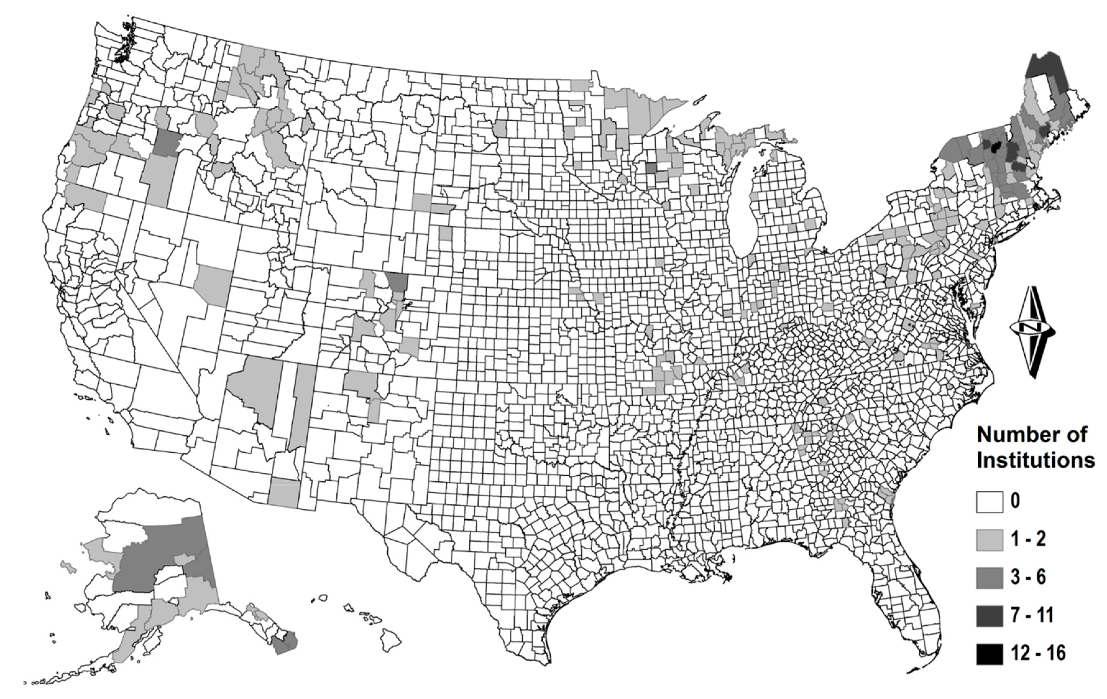
| Institutions | Institutions using biomass heating systems | institutions (count) | Wood2Energy Database, 2014 |
| γ—Zero Inflated (ZI-Binary) | |||
| Heating degree days (HDD) | 1981–2010—Total average heating degree days | HDD (1000) | USA National Oceanic and Atmospheric Administration, 2014 |
| Population density | 2010—Population density | people per km2 | USA Census Bureau, 2013 |
| Forest residue | 2007—logging residues and other removals | m3 (1 × 10⁷) | USDA, USFS Timber Product Output, 2007 |
| β—Negative Binomial (NB-Count) | |||
| Heating degree days (HDD) | 1981–2010—Total average heating degree days | HDD (1000) | USA National Oceanic and Atmospheric Administration, 2014 |
| Natural gas price | 2008–2010—Commercial natural gas three-year average price | USA dollars ($) per 1000 ft3 | USA Energy Information Administration, 2013 |
| House value | 2008–2012—Median value of owner-occupied housing | USA dollars ($) (1000) | USA Census Bureau, 2013 |
| Forest residue | 2007—Logging residues and other removals | m3 (1 × 10⁷) | USDA, USFS Timber Product Output, 2007 |
| Biomass planned removal | 2006–2010—Biomass removal planned in National Fire Plan | m2 (1 × 10⁶) | National Fire Plan Operating and Reporting System, 2006–2010 |
| Federal land | 2005, 2012—Proportion of land managed by Federal Agencies | proportion | National Atlas of the USA and the USA Geological Survey, 2005, 2012 |
| Population | 2010—Population | people (1 × 10⁵) | USA Census Bureau, 2013 |
| Road density | 2013—Primary (interstates) and secondary road (main state and county highways) | m of road per 1000 m2 area | USA Census Bureau, 2013 |
| Port capacity | 2008–2012—Average port capacity of ports | short tons (1 × 10⁵) | USA Army Corps, 2014 |
| County area | 2010—County Area | m2 (1 × 10⁹) | USA Census Bureau, 2013 |
| Total policies | 2011—Total number of state policies that effect forest biomass use directly or indirectly | policies (count) | Becker, Moseley, and Lee, 2011 |
| PM10 historical emissions | 1978–2004—Total number of years county was in PM10 nonattainment | years (count) | USA EPA, 2015 |
| PM10 recent emissions | 2005–2015—Total number of years county was in PM10 nonattainment | years (count) | USA EPA, 2015 |
| PM2.5 recent emissions | 2005–2015—Total number of years county was in PM2.5 nonattainment | years (count) | USA EPA, 2015 |
| SO2 historical emissions | 1978–2004—Total number of years county was in SO2 nonattainment | years (count) | USA EPA, 2015 |
| SO2 recent emissions | 2005–2015—Total number of years county was in SO2 nonattainment | years (count) | USA EPA, 2015 |
| CO2e emissions | 2013—Point Source emissions of greenhouse gases | tonne CO2e | USA EPA, 2013 |
| RPS support | 2015—Local support for RPS | proportion | Howe et al., 2015 |
| Variable | Obs. | Mean | Std. Dev. | Min | Max |
|---|---|---|---|---|---|
| Institutions | 3143 | 0.127585 | 0.675534 | 0 | 16 |
| Heating degree days | 3143 | 4.996686 | 2.191648 | 0.002182 | 19.09467 |
| Population density | 3143 | 1.001250 | 6.657018 | 0 | 268.2155 |
| Natural gas prices | 3143 | 10.43197 | 1.830150 | 7.38 | 35.18666 |
| House value | 3143 | 131.8983 | 80.61617 | 0 | 944.1 |
| Forest residues | 3143 | 2.466242 | 4.632817 | 0 | 70.0118 |
| Biomass NFP | 3143 | 2.415140 | 12.80937 | 0 | 250.9294 |
| Proportion federal lands * | 3143 | 0.126889 | 0.239603 | 0 | 1.062016 |
| Population | 3143 | 0.982328 | 3.129012 | 0.00082 | 98.18605 |
| Road Density | 3143 | 0.204257 | 0.199780 | 0 | 2.650168 |
| Port Capacity | 3143 | 1.013043 | 9.286781 | 0 | 234.2816 |
| County Area | 3143 | 2.910467 | 9.353530 | 0.00518 | 376.8557 |
| Latitude | 3142 | 18.40748 | 63.69796 | −126.638 | 433.3846 |
| Longitude | 3142 | 34.46994 | 104.9199 | −621.637 | 219.9037 |
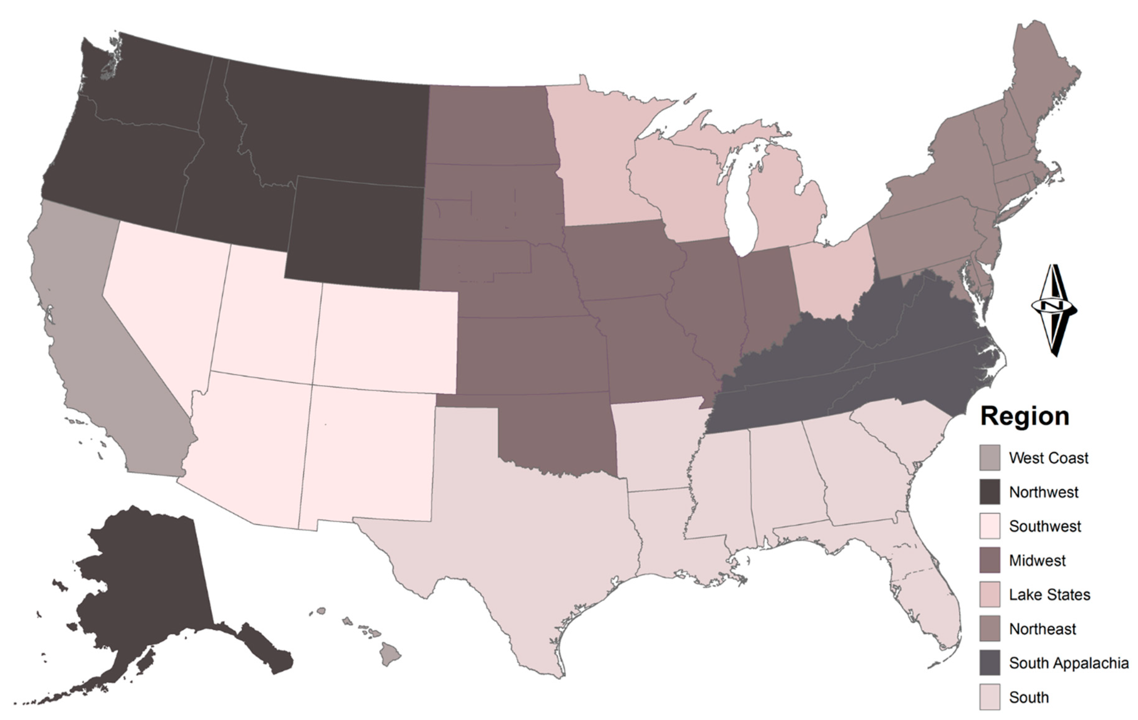
| West Coast | 3143 | 0.020045 | 0.140175 | 0 | 1 |
| South | 3143 | 0.258988 | 0.438149 | 0 | 1 |
| Lake States | 3143 | 0.104995 | 0.306596 | 0 | 1 |
| Northeast | 3143 | 0.077633 | 0.267636 | 0 | 1 |
| Northwest | 3143 | 0.072224 | 0.258900 | 0 | 1 |
| Midwest | 3143 | 0.255170 | 0.436026 | 0 | 1 |
| Southwest | 3143 | 0.050270 | 0.218537 | 0 | 1 |
| Total Policies | 3142 | 7.247295 | 3.757148 | 2 | 15 |
| Cost Share Grants | 3142 | 0.931891 | 1.279653 | 0 | 6 |
| Technical Assistance | 3142 | 1.488542 | 1.570085 | 0 | 6 |
| Financing | 3142 | 0.543921 | 0.675076 | 0 | 3 |
| Procurement | 3142 | 1.305856 | 1.026406 | 0 | 4 |
| Rules and Regulations | 3142 | 1.048695 | 1.222930 | 0 | 3 |
| Tax Incentives | 3142 | 1.928390 | 1.973793 | 0 | 10 |
| PM10 Historical Emissions ** | 3143 | 1.69965 | 4.823705 | 0 | 27 |
| PM10 Recent Emissions ** | 3143 | 0.1384028 | 1.17593 | 0 | 11 |
| PM2.5 Recent Emissions ** | 3143 | 0.6757875 | 2.378869 | 0 | 11 |
| SO2 Historical Emissions ** | 3143 | 0.4492523 | 2.916603 | 0 | 27 |
| SO2 Recent Emissions ** | 3143 | 0.0591791 | 0.609962 | 0 | 11 |
| CO2e Emissions | 3143 | 964279.2 | 2933563 | 0 | 49400820 |
| Proportion of RPS Support *** | 3143 | 0.5809858 | 0.045522 | 0.4499687 | 0.7835159 |
| Dependent: Institutions | Model 1 | Model 2 | ||||||
|---|---|---|---|---|---|---|---|---|
| Independent Variables | Coefficient | OR | Robust | p | Coefficient | OR | Robust | p |
| IRR | SE | IRR | SE | |||||
| Zero Inflated (ZI-Logistic) | ||||||||
| Heating Degree Days | −0.214 * | 0.807 | 0.122 | 0.08 | −0.194 * | 0.824 | 0.107 | 0.07 |
| Population Density | −0.050 * | 0.951 | 0.029 | 0.08 | −0.050 * | 0.951 | 0.029 | 0.09 |
| Forest Residues | −2.111 *** | 0.121 | 0.794 | 0.01 | −2.045 *** | 0.129 | 0.695 | 0.00 |
| _cons | 2.854 *** | 0.903 | 0.00 | 2.666 *** | 0.819 | 0.00 | ||
| Negative Binomial (NB-Count) | ||||||||
| Heating Degree Days | 0.195 * | 1.215 | 0.105 | 0.06 | 0.160 | 1.174 | 0.099 | 0.11 |
| Natural Gas Prices | 0.232 *** | 1.261 | 0.058 | 0.00 | 0.187 *** | 1.206 | 0.066 | 0.00 |
| House Value | 0.002 | 1.002 | 0.001 | 0.13 | 0.001 | 1.001 | 0.001 | 0.39 |
| Forest Residues | 0.001 | 1.001 | 0.007 | 0.90 | 0.000 | 1.000 | 0.007 | 1.00 |
| Biomass NFP | 0.008 ** | 1.008 | 0.004 | 0.04 | 0.009 ** | 1.009 | 0.004 | 0.03 |
| Proportion Federal Land | 0.851 *** | 2.343 | 0.299 | 0.00 | 0.845 *** | 2.329 | 0.289 | 0.00 |
| Population | −0.022 | 0.978 | 0.038 | 0.56 | −0.006 | 0.994 | 0.036 | 0.87 |
| Road Density | −1.302 ** | 0.272 | 0.591 | 0.03 | −1.456 ** | 0.233 | 0.618 | 0.02 |
| Port Capacity | −0.014 * | 0.987 | 0.008 | 0.08 | −0.013 * | 0.987 | 0.007 | 0.07 |
| County Area | 0.001 | 1.001 | 0.002 | 0.71 | 0.001 | 1.001 | 0.001 | 0.56 |
| Latitude | 0.009 *** | 1.009 | 0.003 | 0.01 | 0.009 *** | 1.009 | 0.003 | 0.00 |
| Longitude | 0.009 *** | 1.009 | 0.002 | 0.00 | 0.010 *** | 1.011 | 0.002 | 0.00 |
| West Coast | 1.549 | 4.707 | 1.216 | 0.20 | 1.492 | 4.446 | 1.224 | 0.22 |
| South | 1.039 ** | 2.828 | 0.450 | 0.02 | 0.650 | 1.916 | 0.429 | 0.13 |
| Lake States | 1.240 *** | 3.456 | 0.413 | 0.00 | 1.092 ** | 2.980 | 0.431 | 0.01 |
| Northeast | 1.161 *** | 3.192 | 0.387 | 0.00 | 1.024 ** | 2.785 | 0.467 | 0.03 |
| Northwest | 2.730 *** | 15.333 | 0.676 | 0.00 | 2.983 *** | 19.755 | 0.716 | 0.00 |
| Midwest | 1.821 *** | 6.180 | 0.457 | 0.00 | 1.483 *** | 4.405 | 0.409 | 0.00 |
| Southwest | 3.686 *** | 39.868 | 0.652 | 0.00 | 3.646 *** | 38.336 | 0.642 | 0.00 |
| Total Policies | −0.049 ** | 0.953 | 0.025 | 0.05 | ||||
| Cost Share Grants | −0.101 | 0.904 | 0.096 | 0.29 | ||||
| Technical Assistance | −0.003 | 0.997 | 0.063 | 0.97 | ||||
| Financing | 0.109 | 1.115 | 0.129 | 0.40 | ||||
| Procurement | −0.332 *** | 0.717 | 0.110 | 0.00 | ||||
| Rules and Regulations | 0.052 | 1.054 | 0.080 | 0.51 | ||||
| Tax Incentives | −0.118 *** | 0.888 | 0.045 | 0.01 | ||||
| PM10 Historical Emissions | 0.016 | 1.016 | 0.015 | 0.28 | 0.012 | 1.012 | 0.015 | 0.41 |
| PM10 Recent Emissions | 0.013 | 1.013 | 0.045 | 0.77 | 0.033 | 1.034 | 0.047 | 0.48 |
| PM2.5 Recent Emissions | 0.007 | 1.007 | 0.034 | 0.83 | 0.006 | 1.006 | 0.035 | 0.86 |
| SO2 Historical Emissions | 0.027 | 1.027 | 0.020 | 0.19 | 0.028 | 1.029 | 0.019 | 0.15 |
| SO2 Recent Emissions | 0.017 | 1.018 | 0.108 | 0.87 | 0.008 | 1.008 | 0.093 | 0.93 |
| CO2e Emissions | −0.000 | 1.000 | 0.000 | 0.40 | −0.000 | 1.000 | 0.000 | 0.57 |
| RPS Support | 6.913 *** | 1005.638 | 1.837 | 0.00 | 7.512 *** | 1829.667 | 1.825 | 0.00 |
| cons | −11.656 *** | 1.447 | 0.00 | −10.904 *** | 1.463 | 0.00 | ||
| lnalpha cons | −0.604 * | 0.340 | 0.08 | −0.766 ** | 0.357 | 0.03 | ||
| alpha cons | 0.546 *** | 0.186 | 0.00 | 0.465 *** | 0.166 | 0.01 | ||
| N | 3142 | 3142 | ||||||
| Log Likelihood | −783.66 | −776.67 | ||||||
| Chi Square | 524.44 | 626.96 | ||||||
| % correctly predicted ± 0.499 residual | 92.08% | 92.27% | ||||||
| Vuong Test a ZINB vs. NB | Likelihood Ratio Test b ZINB vs. ZIP | |||
|---|---|---|---|---|
| Statistic (V c) | p-Value | Statistic (z-score) | p-Value | |
| Model 1 | 4.18 | <0.0001 | 29.31 | <0.0001 |
| Model 2 | 4.16 | <0.0001 | 24.79 | <0.0001 |
| Institutions | Actual | Predicted | Difference |
|---|---|---|---|
| Model 1 | |||
| 0 | 92.84% | 92.92% | −0.08% pts. |
| 1 | 04.87% | 04.90% | −0.03% pts. |
| 2 | 01.15% | 01.11% | 0.04% pts. |
| 3 | 00.60% | 00.42% | 0.18% pts. |
| 4 | 00.16% | 00.22% | −0.06% pts. |
| 5 | 00.06% | 00.13% | −0.07% pts. |
| Model 2 | |||
| 0 | 92.84% | 92.94% | −0.10% pts. |
| 1 | 04.87% | 04.91% | −0.04% pts. |
| 2 | 01.15% | 01.08% | 0.07% pts. |
| 3 | 00.60% | 00.41% | 0.19% pts. |
| 4 | 00.16% | 00.21% | −0.05% pts. |
| 5 | 00.06% | 00.13% | −0.07% pts. |
| Likelihood Ratio Test | d.f. | Chi Squared | p-Value |
|---|---|---|---|
| Model 1 nested in Model 2 | 5 | 13.98 * | 0.0157 |
© 2018 by the authors. Licensee MDPI, Basel, Switzerland. This article is an open access article distributed under the terms and conditions of the Creative Commons Attribution (CC BY) license (http://creativecommons.org/licenses/by/4.0/).
Share and Cite
Young, J.D.; Anderson, N.M.; Naughton, H.T. Influence of Policy, Air Quality, and Local Attitudes toward Renewable Energy on the Adoption of Woody Biomass Heating Systems. Energies 2018, 11, 2873. https://0-doi-org.brum.beds.ac.uk/10.3390/en11112873
Young JD, Anderson NM, Naughton HT. Influence of Policy, Air Quality, and Local Attitudes toward Renewable Energy on the Adoption of Woody Biomass Heating Systems. Energies. 2018; 11(11):2873. https://0-doi-org.brum.beds.ac.uk/10.3390/en11112873
Chicago/Turabian StyleYoung, Jesse D., Nathaniel M. Anderson, and Helen T. Naughton. 2018. "Influence of Policy, Air Quality, and Local Attitudes toward Renewable Energy on the Adoption of Woody Biomass Heating Systems" Energies 11, no. 11: 2873. https://0-doi-org.brum.beds.ac.uk/10.3390/en11112873