Phase-Locked Loop Research of Grid-Connected Inverter Based on Impedance Analysis

Abstract

In order to improve the phenomenon that a traditional phase-locked loop based on a double second-order generalized integrator (DSOGI-PLL) cannot track signal amplitude and phase accurately when the input signal contains DC components and high-order harmonics, the structure of a second-order generalized integrator-quadrature signals generator (SOGI-QSG) is modified. The paper establishes the impedance model considering the DSOGI-PLL structure of the inductor-capacitor-inductor-type (LCL-type) inverter grid-connected system adopting current control measured from the grid terminal in alternating current side, introducing voltage feedback control to enhance the stability of the system. Meanwhile, analyzing the influence of parameters on impedance according to the impedance model established preferable design parameters. The improvement in SOGI-QSG structure is good for PLL to lock the grid voltage phase more accurately and the retrofitting in control strategy based on the impedance is able to uplift the inverter output impedance phase which is conducive to system stability by increasing the phase margin of the system. The simulation in Matlab/Simulink is carried out to verify the effectiveness of the proposed control strategy.

1. Introduction

The grid is a complex dynamic system originally. For controlling the current and grid voltage to obtain synchronization, it is indispensable to detect the variation of phase and frequency with grid voltage accurately and quickly. In addition, the explosive development of renewable energy, that is, wind and solar, results in the proportion of power electronic equipment in traditional power grid increasing gradually, such as grid-connected inverters, reactive compensators and other equipment, which brings a lot of new problems to the grid [1,2,3], as well as increasing the difficulty to lock phase for phase-locked loop (PLL). There are two main schemes to realize the phase-locking, one based on PLL [4,5] that the paper focuses on and another without PLL [6,7] for the purpose of frequency tracking and phase locking of the gird. PLL is used to implement synchronization between the control loop and the grid system, however, a large amount of penetration of distributed generation systems in the grid will inevitably give rise to the grid system stability problem. Therefore, it is fairly necessary to research the phase-locked loop in order to ensure the system does not lose stability because of the phase synchronous problem.

In view of the PLL as an indispensable part of grid-connected system, scholars have always insisted on researching it to improve the performance of PLL. Synchronous reference frame-phase locked loop (SRF-PLL) is a common phase-locked way [8,9] due to simple control mode and fast response speed. However, if the conditions of voltage unbalance and high-order harmonics resulting from grid fault appear, SRF-PLL will have a larger error in phase locking. In light of decoupled double synchronous reference frame-PLL (DDSRF-PLL) [10] utilizing the decoupling network to eliminate the double harmonics caused by the negative sequence component, a good result of phase lock is obtained [11,12,13]. However, the method has a large amount of computation and slow dynamic response. Besides, the low pass filter will generate delay to some extent that may affect the real-time performance of the control. Whereas the second-order generalized integrator-PLL (DSOGI-PLL) can effectively deal with the inaccurate phase-locking problem of DDSRF-PLL under an unbalanced grid voltage fault. However, the phase-locked information cannot be accurately obtained under the condition of DC voltage and high harmonics included in the grid voltage. In [14] Xie et al. compare systematically the seven advanced phase locking method based on the second-order generalized integrator (SOGI) in the inhibition capacity of DC bias, including the cascade SOGI, modified SOGI, αβ-frame delayed signal cancellation (DSC), complex coefficient filter, in-loop dq-frame DSC, notch filter and moving average filter-based SOGI-PLL. However, the paper only considers the phase synchronization capacity of the PLL under DC bias without considering other conditions, such as three-phase unbalance of grid voltage; Jin et al. in [15] proposes an adaptive filter based on SOGI to extract the positive and negative sequence of three-phase grid voltage, aiming at the tracking error generated by traditional PLL under harmonic distortion and grid asymmetry. However, the paper cannot explain detailed analysis on the PLL model. In allusion to the phenomenon that the traditional DSOGI-PLL cannot lock phase precisely when the DC components and high order harmonics are contained in the grid voltage, the paper proposes the improved second-order generalized integrator-quadrature signals generator (SOGI-QSG) structure. The SOGI-QSG is a significant part of the DSOGI-PLL. The grid voltage is transformed by Clark transform to be the input signal of the SOGI-QSG. The SOGI-QSG output signal is mutually orthogonal signals. Processing positive sequence q-axis signal can realize phase lock after the positive and negative sequence separation about SOGI-QSG output signals. The asymmetric three-phase voltage can be decomposed into positive sequence, negative sequence and zero sequence components by symmetrical component method. To extract the positive sequence component of the grid voltage signal, the phase offset signal of the original signal is necessary, that is, two phase orthogonal signals. It is important for DSOGI-PLL to analyze the SOGI-QSG characteristics and improve the SOGI-QSG structure.

The research on the stability of grid-connected LCL-type inverters is often based on the impedance model, which greatly simplifies the analysis complexity. Simultaneously, impedance stability criterion can be directly employed to evaluate the grid-connected system stability. Liu et al. in [16] proposes the control strategy of optimization delay aiming to solving the problem that the control path calculation delay is not conductive to the system stability under the current control mode of LCL-type grid-connected inverter. The strategy is effective to improve the system stability. In [17] Schiesser et al. proposes a simplified proportion multi-resonant (PMR) current controller tuning strategy considering grid-connected stability which effectively improves the current harmonic distortion, aiming to solve the problem of low frequency harmonics caused by the grid voltage distortion or the non-linear characteristics of current loop in the grid-connected voltage source inverter (VSI). Xin et al. in [18] puts forward the inverter-side current feedback (ICF) without additional sensors to control the system harmonic, aiming to solving the problem that grid-connected current of LCL-type grid-connected inverter is vulnerable to the grid harmonic distortion. However, this method needs to use the resonant controller and additional compensation loop at the same time. Wen et al. in [19] set up the small signal impedance model of three-phase grid-connected inverter considering feedback control and DDSRF-PLL in d-q coordinate. Based on the impedance, the influence of PLL, current loop and power loop on the inverter is discussed, and the influence of bandwidth in PLL on the system stability also is analyzed. The paper only establishes and analyzes the impedance model of an L-type grid-connected inverter based on small signal method without other simulation about control strategies. Zeng et al. in [20] propose a novel impedance control strategy to reshape the output impedance of the PV grid-connected inverter in order to suppress the harmonic resonance phenomenon in the PV grid-connected system. For the aforementioned acumen, in [21] Chen et al. studies the interaction between PV inverter and grid based on the impedance analysis. Active impedance control strategy based on voltage feedforward is proposed, so that the grid-connected inverter has better control robustness under different dynamic gird conditions. In [22] Wu et al. deduces the stability criterion of a grid-connected inverter system considering PLL under different grid conditions, taking a single-phase LCL-type grid-connected inverter as an example. Meanwhile, the influence of PLL on the stability of single-phase LCL-type grid-connected inverter is also analyzed in detail, and the method of PLL parameter design based on the requirement of phase angle margin is proposed. For improving the stability of LCL-type grid-connected inverter, the output impedance model of LCL-type grid-connected inverter considering DSOGI-PLL structure is established. Meanwhile, the system phase margin at the impedance intersection is raised by introducing compensated grid-connected voltage into the current loop, thereby enhancing the system stability. The paper conducts research on the basis of three-phase LCL-type grid-connected inverter under the grid-connected current control mode. Aiming at the phenomenon that the traditional PLL cannot realize precise synchronization in the gird fault, the improved SOGI-QSG structure is presented, which can realize precise phase-locking in the grid fault, such as the unbalanced grid, DC components and harmonic included in the grid voltage. Meanwhile, the voltage feedback control strategy is introduced to raise the system stability based on impedance analysis. Firstly, an improved DSOGI-PLL is proposed to solve the problem that the original DSOGI-PLL cannot accurately lock the phase when the DC component included. Then, the output impedance mathematical model of LCL-type grid-connected inverter considering PLL is established and the stability of grid-connected inverter is analyzed based on the cascade stability criterion of impedance [23,24]. At last, the design parameters of improved SOGI-QSG structure and control strategy are displayed, which is verified by simulation. Simulation results show that the accuracy of improved PLL output frequency and the voltage and current characteristics of grid-connection are improved effectively.

2. Impedance Model

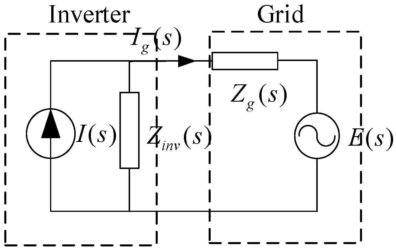
Figure 1 is the equivalent circuit of LCL-type inverter grid-connected system. The inverter adopts grid side current closed loop control mode.

Where Z_inv(s) is the equivalent output impedance of the inverter AC terminal; Z_g(s) is the equivalent impedance of the grid; I(s) is the equivalent current source of the inverter; E(s) is the ideal grid voltage source. Equation (1) is the expression of grid current I_g(s).

$$I_g(s)=\left[I(s)-E(s)Z_{inv}^{-1}(s)\right]{\left[Z_g(s)Z_{inv}^{-1}(s)+E\right]}^{-1}$$

(1)

where E denotes identity matrix.

In order to ensure the system stability under the conditions of impedance variation, the following two terms must be satisfied [25]: (1) when the grid impedance is equal to zero, the system is stable; and (2) when the grid impedance exists, Z_g(s)$Z_{inv}^{-1}$(s) needs to satisfy the impedance stability criterion. According to the Equation (1), the whole grid-connected system will be stable if the above terms can be satisfied at the same time. Then, the inverter output impedance and grid impedance are modeled respectively.

2.1. Grid Connected Inverter Model

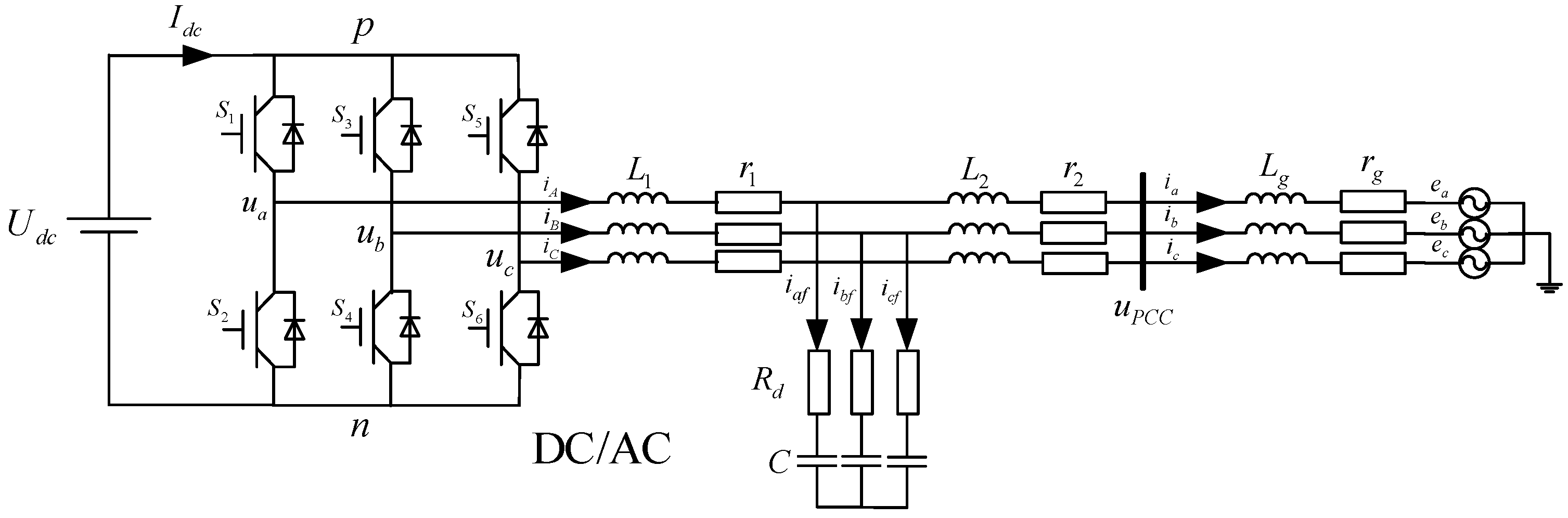
A LCL-type grid-connected inverter can availably suppress the high-order harmonics of the grid current, while the grid inductance can also play a role in suppressing the impulse current. Figure 2 is the grid-connected inverter topology which contains a LCL-type filter.

Where U_dc and I_dc represent DC link voltage and current respectively; L₁, r₁ represent the machine-side filter inductance and inductance parasitic resistance respectively; L₂, r₂ represent the grid-side filter inductance and inductance parasitic resistance respectively; R_d represents the damping resistance; C is the filter capacitance; L_g, r_g represent the equivalent inductance and resistance of electric wires respectively; and e_i (I = a,b,c) represents the ideal three-phase grid voltage.

Equation (2) is the state-space equation of grid-connected inverter in three-phase stationary coordinates.

$$\{\begin{array}{l}\left[\begin{array}{c}{u}_a\\ u_b\\ u_c\end{array}\right]=L_1\frac{d}{dt}\left[\begin{array}{c}{i}_A\\ i_B\\ i_C\end{array}\right]+r_1\left[\begin{array}{c}{i}_A\\ i_B\\ i_C\end{array}\right]+L_2\frac{d}{dt}\left[\begin{array}{c}{i}_a\\ i_b\\ i_c\end{array}\right]+r_2\left[\begin{array}{c}{i}_a\\ i_b\\ i_c\end{array}\right]+\left[\begin{array}{c}{u}_{ga}\\ u_{gb}\\ u_{gc}\end{array}\right]\\ \begin{array}{l}C\frac{d}{dt}\left[\begin{array}{c}{u}_{afc}\\ u_{bfc}\\ u_{cfc}\end{array}\right]=\left[\begin{array}{c}{i}_A\\ i_B\\ i_C\end{array}\right]-\left[\begin{array}{c}{i}_a\\ i_b\\ i_c\end{array}\right]\\ R_{d}C\frac{d}{dt}\left[\begin{array}{c}{u}_{afc}\\ u_{bfc}\\ u_{cfc}\end{array}\right]+\left[\begin{array}{c}{u}_{afc}\\ u_{bfc}\\ u_{cfc}\end{array}\right]=L_2\frac{d}{dt}\left[\begin{array}{c}{i}_a\\ i_b\\ i_c\end{array}\right]+r_2\left[\begin{array}{c}{i}_a\\ i_b\\ i_c\end{array}\right]+\left[\begin{array}{c}{u}_{ga}\\ u_{gb}\\ u_{gc}\end{array}\right]\end{array}\end{array}$$

(2)

where u_i, u_gi (I = a,b,c) represent the three-phase voltage at the machine side and the grid side respectively; i_i (I = A,B,C), i_i (I = a,b,c) represent the three-phase current at the machine side and grid side respectively; and u_ifc (I = a,b,c) represents the capacitor terminal voltage.

The main circuit small signal simplified model is shown as Equation (3) obtained by analyzing Equation (2) with Laplace transform and the small signal analysis method.

$$\left[\begin{array}{l}{\widehat{i}}_d\\ {\widehat{i}}_q\end{array}\right]=-B^{-1}A\left[\begin{array}{l}{\widehat{u}}_{gd}\\ {\widehat{u}}_{gq}\end{array}\right]+B^{-1}{U}_{dc}\left[\begin{array}{l}{\widehat{d}}_d\\ {\widehat{d}}_q\end{array}\right]+B^{-1}\left[\begin{array}{l}{D}_d\\ D_q\end{array}\right]{\widehat{u}}_{dc}=G_{g^{\prime }}\left[\begin{array}{l}{\widehat{u}}_{gd}\\ {\widehat{u}}_{gq}\end{array}\right]+G_{gI}\left[\begin{array}{l}{\widehat{d}}_d\\ {\widehat{d}}_q\end{array}\right]+B^{-1}\left[\begin{array}{l}{D}_d\\ D_q\end{array}\right]{\widehat{u}}_{dc}$$

(3)

where ${\widehat{i}}_i、{\widehat{u}}_{gi}、{\widehat{d}}_i\hspace{0.17em}(i=d,q)$ represent current, voltage and duty ratio small signal perturbation on d-q axis in grid side respectively; D_i (I = d,q) represents duty ratio in steady state on d-q axis; ${\widehat{u}}_{dc}$ represents the DC link voltage small signal perturbation; G_g’ represents the grid-connected inverter output admittance; and G_gI represents the duty ratio to the grid side current transfer function.

Equations (4) and (5) denote the expressions of A and B respectively.

$$A=\left[\begin{array}{cc}s{L}_1+r_1& -{\omega }^{\prime }{L}_1\\ {\omega }^{\prime }{L}_1& s{L}_1+r_1\end{array}\right]\left[\begin{array}{cc}sC& -{\omega }^{\prime }C\\ {\omega }^{\prime }C& sC\end{array}\right]{\left[\begin{array}{cc}s{R}_{d}C+1& -{\omega }^{\prime }{R}_{d}C\\ {\omega }^{\prime }{R}_{d}C& s{R}_{d}C+1\end{array}\right]}^{-1}+I$$

(4)

$$\begin{array}{ll}B=& \left[\begin{array}{cc}s{L}_1+r_1& -{\omega }^{\prime }{L}_1\\ {\omega }^{\prime }{L}_1& s{L}_1+r_1\end{array}\right]+\left[\begin{array}{cc}s{L}_1+r_1& -{\omega }^{\prime }{L}_1\\ {\omega }^{\prime }{L}_1& s{L}_1+r_1\end{array}\right]\left[\begin{array}{cc}sC& -{\omega }^{\prime }C\\ {\omega }^{\prime }C& sC\end{array}\right]\ast \\ & {\left[\begin{array}{cc}s{R}_{d}C+1& -{\omega }^{\prime }{R}_{d}C\\ {\omega }^{\prime }{R}_{d}C& s{R}_{d}C+1\end{array}\right]}^{-1}\left[\begin{array}{cc}s{L}_2+r_2& -{\omega }^{\prime }{L}_2\\ {\omega }^{\prime }{L}_2& s{L}_2+r_2\end{array}\right]+\left[\begin{array}{cc}s{L}_2+r_2& -{\omega }^{\prime }{L}_2\\ {\omega }^{\prime }{L}_2& s{L}_2+r_2\end{array}\right]\end{array}$$

(5)

where ω′ is the PLL output angular frequency.

The derivation of grid small signal model is similar to the grid-connected inverter. Equation (6) is the grid state-space equation in three-phase stationary coordinates.

$$\left[\begin{array}{c}{u}_{ga}\\ u_{gb}\\ u_{gc}\end{array}\right]=L_g\frac{d}{dt}\left[\begin{array}{c}{i}_a\\ i_b\\ i_c\end{array}\right]+r_g\left[\begin{array}{c}{i}_a\\ i_b\\ i_c\end{array}\right]+\left[\begin{array}{c}{e}_a\\ e_b\\ e_c\end{array}\right]$$

(6)

The following Equation (7) showing the grid small signal model is received by transforming the Equation (6) with park transformation and small signal analysis method.

$$\left[\begin{array}{l}{\widehat{u}}_{gd}\\ {\widehat{u}}_{gq}\end{array}\right]=\left[\begin{array}{cc}s{L}_g+r_g& -{\omega }^{\prime }{L}_g\\ {\omega }^{\prime }{L}_g& s{L}_g+r_g\end{array}\right]\left[\begin{array}{l}{\widehat{i}}_d\\ {\widehat{i}}_q\end{array}\right]+\left[\begin{array}{l}{\widehat{e}}_d\\ {\widehat{e}}_q\end{array}\right]$$

(7)

where ${\widehat{e}}_i(i=d,q)$ represent grid voltage small signal perturbation on d-q axis.

2.2. Phase-Locked Loop Model

2.2.1. Traditional Second-Order Generalized Integrator-Quadrature Signals Generator Structure

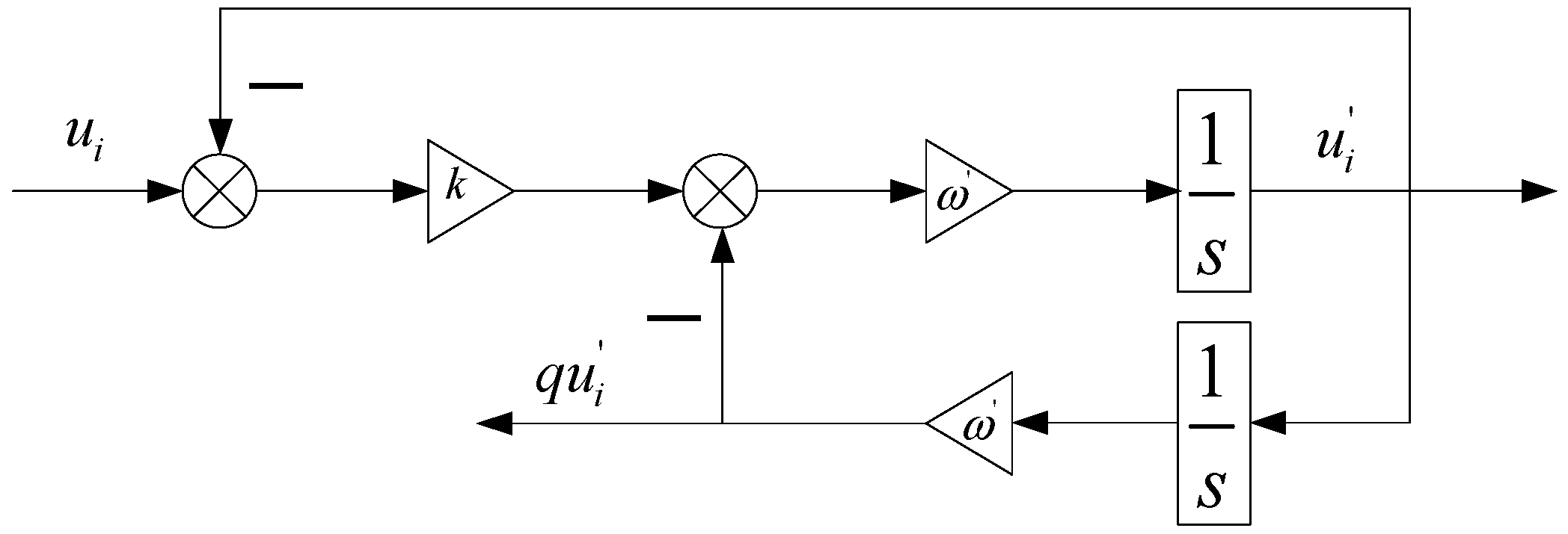
Figure 3 is the traditional SOGI-QSG structure. The quadrature signal generator based on the traditional second-order generalized integrator (SOGI) not only can realize 90° phase angle offset of input signal, but also filter out high-order harmonics.

In Figure 3, u_i is the input signal and $u_I^{\prime }$, ${qu}_I^{\prime }$ are SOGI-QSG output signals that are two orthogonal signals; k is the damping coefficient; ω′ is the PLL output angular frequency. Equations (8) and (9) denote the characteristic transfer functions of the SOGI-QSG.

$$D_1(s)=\frac{u_i^{\prime }}{u_i}=\frac{k{\omega }^{\prime }s}{s^2+k{\omega }^{\prime }s+{\omega }^{\prime }{}^2}$$

(8)

$$Q_1(s)=\frac{q{u}_i^{\prime }}{u_i}=\frac{k{\omega }^{\prime }{}^2}{s^2+k{\omega }^{\prime }s+{\omega }^{\prime }{}^2}$$

(9)

2.2.2. Improved Second-Order Generalized Integrator-Quadrature Signals Generator Structure

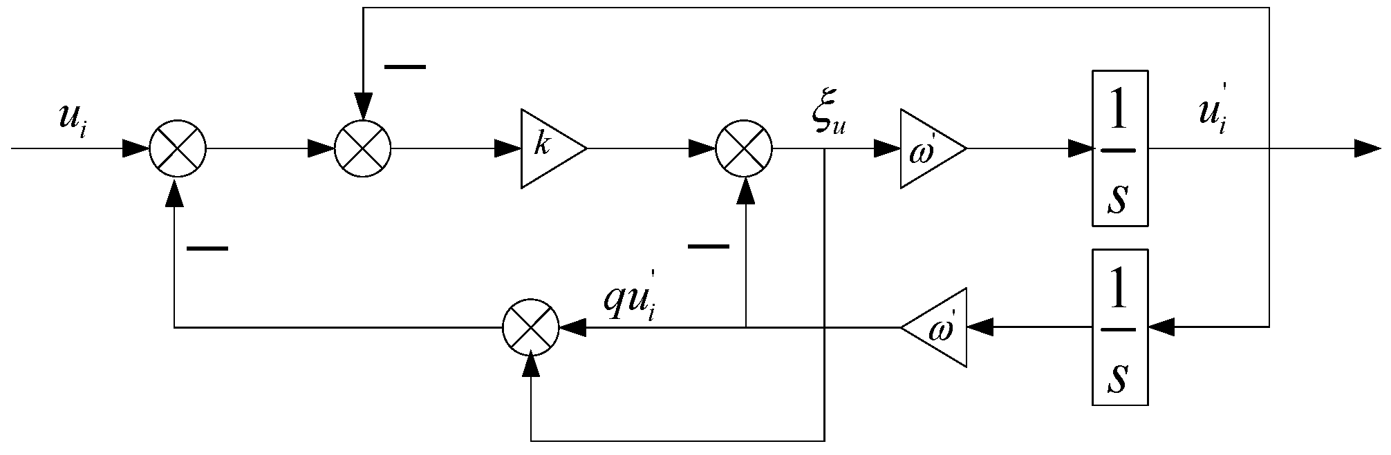
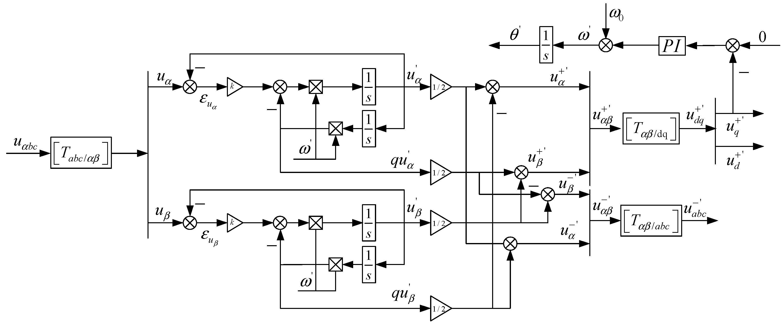
Because ${qu}_i^{\prime }$ cannot suppress the dc component included in the input signals in the traditional SOGI structure, the improved SOGI-QSG structure is proposed shown in Figure 4.

Equations (11) and (12) are the SOGI-QSG transfer functions after introducing feedback.

$$F(s)=\frac{{\xi }_u}{u_i}=\frac{k{s}^2}{s^2+k{\omega }^{\prime }s+{{\omega }^{\prime }}^2}$$

(10)

$$D_2(s)=\frac{u_i^{\prime }}{u_i}=\frac{k{\omega }^{\prime }s}{(k+1)s^2+k{\omega }^{\prime }s+(k+1){\omega }^{\prime }{}^2}$$

(11)

$$Q_2(s)=\frac{q{u}_i^{\prime }}{u_i}=\frac{k{\omega }^{\prime }{}^2}{(k+1)s^2+k{\omega }^{\prime }s+(k+1){\omega }^{\prime }{}^2}$$

(12)

where F(s) is the high-pass filter and Q₂(s) is the low-pass filter. The dc component and high-order harmonics input to the SOGI-QSG are weakened by feeding back F(s) and Q₂(s) to the input signals. It is conducive to reducing the phase locking error.

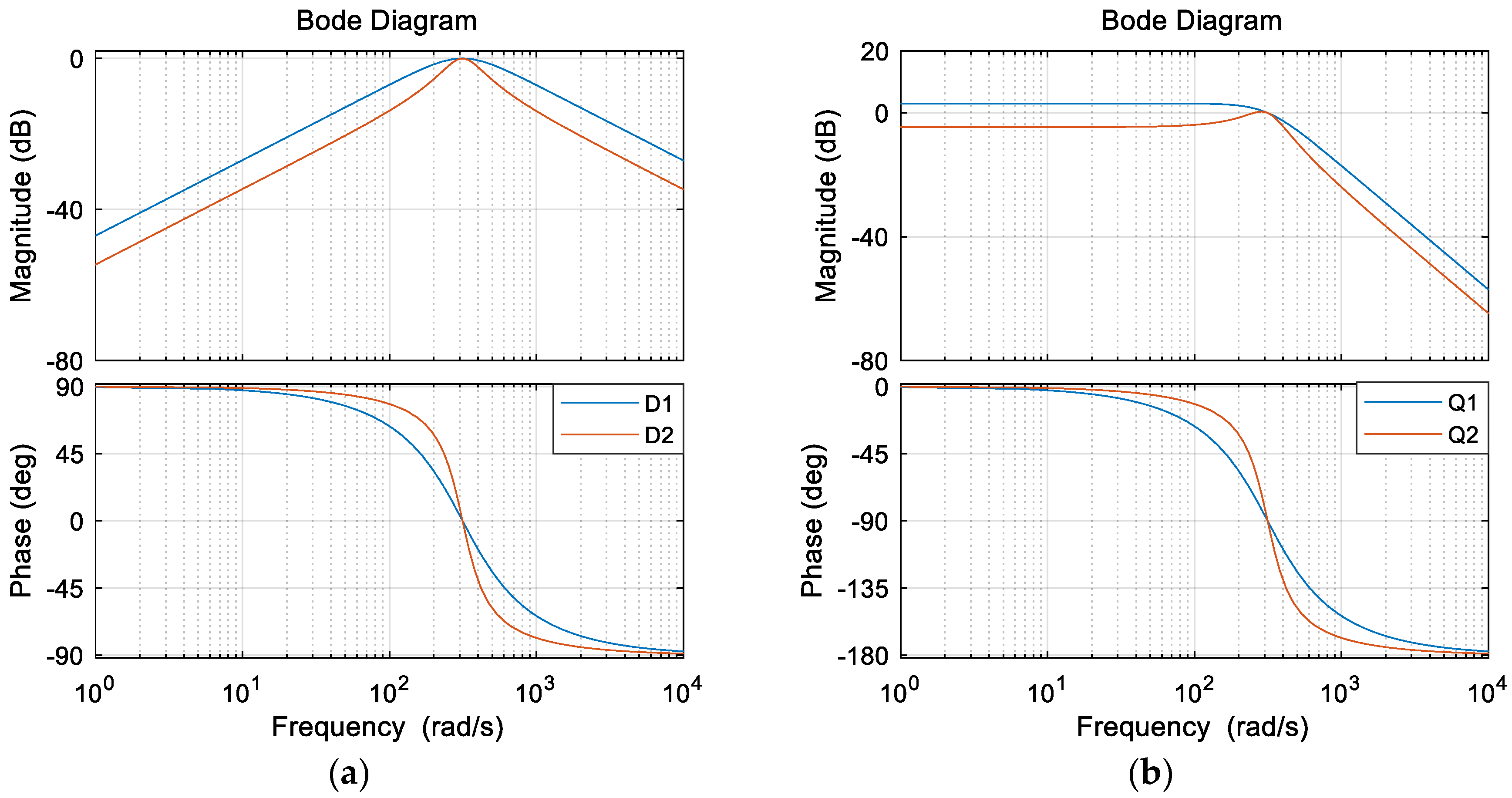
Figure 5 shows the comparison of SOGI-QSG transfer function bode plot before and after PLL improvement. Obviously, the bandwidth of the improved SOGI-QSG is reduced and the filtering characteristic is enhanced. However, its dynamic performance is worse and the adjustment time is slightly longer.

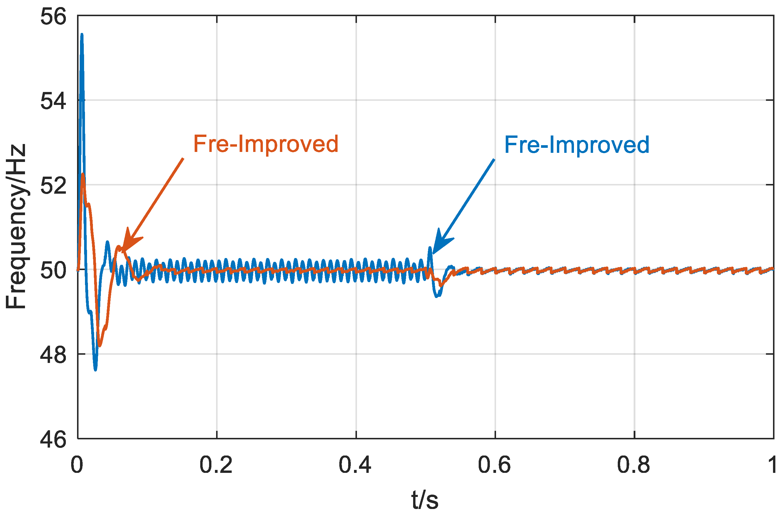
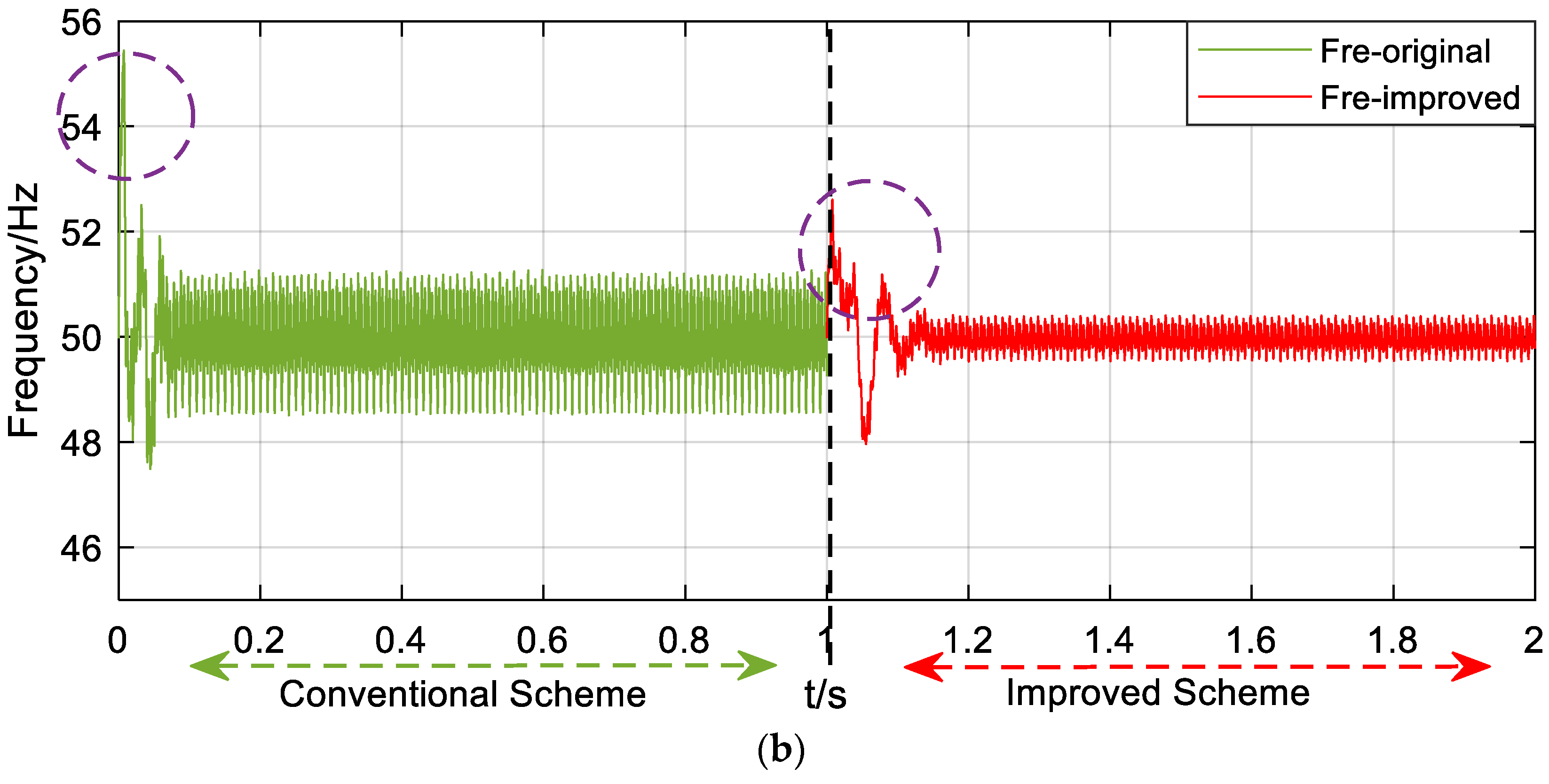
Figure 6 shows the PLL output frequency waveform when the grid-connected voltage surges by 30%. The orange and light blue curves represent the PLL frequency output waveform of SOGI-QSG structure before and after improvement respectively. It can be seen from the Figure that the frequency fluctuation of improved SOGI-QSG structure is obviously reduced in the steady state, which indicates that the filtering effect of the improved structure is indeed greatly raised, however, it is not very good in the transient state. This is reasonable because the bandwidth of the improved SOGI-QSG transfer function decreases. The improved structure raises filtering performance at the expense of its dynamic characteristic. Therefore, the adjustment time is longer than the original structure output in the transient process. It also can be seen in the Figure that the dynamic response time of the improved SOGI-QSG output frequency has slightly increased, which has little impact on the overall performance of the structure compared with the improvement on filtering.

2.3. Inverter Impedance Model

2.3.1. Inverter Impedance Model without Feedback Control

As Figure 7 shows, the DSOGI-PLL structure, the positive sequence q-axis signal which removed from SOGI output signal by positive and negative sequence separation, is processed to realize phase-locked. Equation (13) is the positive sequence signal expression under α-β coordinates.

$$\left[\begin{array}{l}{u}_{\alpha }^{+\prime }\\ u_{\beta }^{+\prime }\end{array}\right]=\frac{1}{2}\left[\begin{array}{cc}1& -q\\ q& 1\end{array}\right]\left[\begin{array}{l}{u}_{\alpha }^{\prime }\\ u_{\beta }^{\prime }\end{array}\right]=\frac{1}{2}\left[\begin{array}{cc}D(s)& -Q(s)\\ Q(s)& D(s)\end{array}\right]\left[\begin{array}{l}{u}_{\alpha }\\ u_{\beta }\end{array}\right]=\left[\begin{array}{cc}{P}_{11}& P_{12}\\ P_{21}& P_{22}\end{array}\right]\left[\begin{array}{l}{u}_{\alpha }\\ u_{\beta }\end{array}\right]$$

(13)

where D(s), Q(s) are used to represent SOGI-QSG transfer function before and after improvement of SOGI-QSG, namely D₁(s)/D₂(s) and Q₁(s)/Q₂(s); Matrix P is used to represent the previous matrix; q = e^−jπ2 is a 90° lagging phase-shifting operator applied on the time domain to obtain an in-quadrature version of the input waveform.

There are two kinds of coordinates in the whole system due to exist in PLL. One is the system d-q coordinate defined by the grid voltage and another is the control loop d-q coordinate defined by the PLL. Under a steady state, the control loop d-q coordinate is consistent with the system d-q coordinate. When a small disturbance happens in the grid voltage terminal, the system d-q coordinate position will be changed. The control loop d-q coordinate has not changed because the dynamic response characteristics of the PI controller in PLL which is no longer consistent with the system d-q coordinate. There is an angle error between the two coordinates, that is ∆θ. Equation (14) denotes the coordinate transformation of the system d-q coordinate the control loop d-q coordinate.

$$T_{\Delta \theta }=\left[\begin{array}{cc}\cos (\Delta \theta )& \sin (\Delta \theta )\\ -\sin (\Delta \theta )& \cos (\Delta \theta )\end{array}\right]$$

(14)

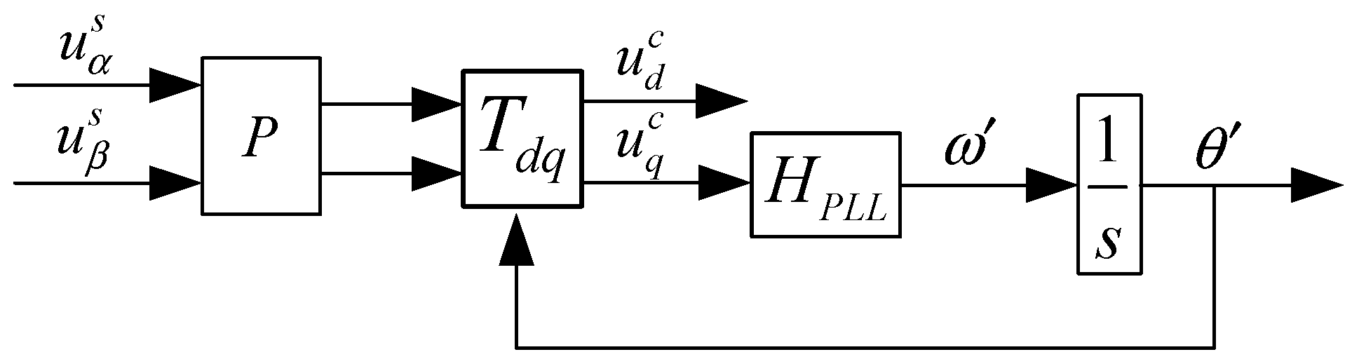
Figure 8 and Figure 9 represent the DSOGI-PLL control strategy and the DSOGI-PLL average model respectively.

Equation (15) denotes the variables relationship between the system and the control loop under the steady-state condition when ∆θ = 0.

$$\begin{array}{c}{U}^c=P{T}_{\Delta \theta }{U}^s=P\left[\begin{array}{cc}\cos (0)& \sin (0)\\ -\sin (0)& \cos (0)\end{array}\right]U^s\\ I^c=P{T}_{\Delta \theta }{I}^s=P\left[\begin{array}{cc}\cos (0)& \sin (0)\\ -\sin (0)& \cos (0)\end{array}\right]I^s\\ D^s={(P{T}_{\Delta \theta })}^{-1}{D}^c=\left[\begin{array}{cc}\cos (0)& -\sin (0)\\ \sin (0)& \cos (0)\end{array}\right]P^{-1}{D}^c\end{array}$$

(15)

where x^c (x = U, I, D) represents the variables in the system’s main circuit; x^s (x = U, I, D) represents the control loop variables. Equation (16) is obtained by adding a small signal disturbance to Equation (15).

$$\left[\begin{array}{l}{U}_d^c+{\tilde{u}}_d^c\\ U_q^c+{\tilde{u}}_q^c\end{array}\right]=P\left[\begin{array}{cc}\cos (0+\Delta \theta )& \sin (0+\Delta \theta )\\ -\sin (0+\Delta \theta )& \cos (0+\Delta \theta )\end{array}\right]\left[\begin{array}{l}{U}_d^s+{\tilde{u}}_d^s\\ U_q^s+{\tilde{u}}_q^s\end{array}\right]$$

(16)

where ${\tilde{u}}_i^c(i=d,q)$ represents the small signal voltage disturbance of main circuit in d-q axis; ${\tilde{u}}_i^s(i=d,q)$ represents the small signal voltage disturbance of control loop in d-q axis.

Equation (17) denotes the voltage expression under the control loop d-q coordinate obtained by handling Equation (16) with trigonometric function approximation method in combination with the steady state condition.

$$\left[\begin{array}{l}{\tilde{u}}_d^c\\ {\tilde{u}}_q^c\end{array}\right]\approx \left[\begin{array}{l}{P}_{11}{\tilde{u}}_d^s-P_{12}\Delta \theta U_d^s+P_{11}{U}_q^s\Delta \theta +P_{12}{\tilde{u}}_q^s\\ P_{21}{\tilde{u}}_d^s-P_{22}{U}_d^s\Delta \theta +P_{21}{U}_q^s\Delta \theta +P_{22}{\tilde{u}}_q^s\end{array}\right]$$

(17)

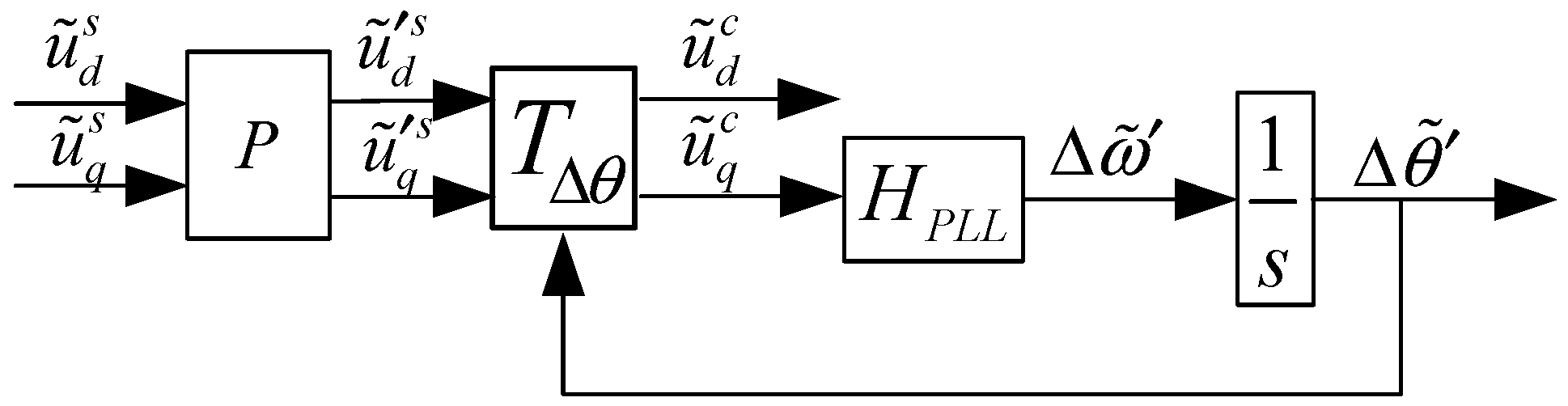
According to the DSOGI-PLL average model in Figure 8, PLL output angle ∆θ can be written as Equation (18).

$$\Delta \theta ={\tilde{u}}_q^c{H}_{PLL}\frac{1}{s}$$

(18)

where H_PLL = k_{PLL_p} + k_{PLL_i}/s; k_{PLL_p} is the proportional coefficient of PI regulator in PLL; k_{PLL_i} is the integral coefficient of PI regulator in PLL. Equation (19), that ∆θ is expressed by ${\tilde{u}}_d^s$ and ${\tilde{u}}_q^s$, is received by substituting Equation (17) into Equation (18).

$$\Delta \theta =G_{PLL1}{\tilde{u}}_d^s+G_{PLL2}{\tilde{u}}_q^s$$

(19)

The G_PLL1 and G_PLL2 in the Equation (19) can be expressed as

$$G_{PLL1}=\frac{\Delta \theta }{{\widehat{u}}_d^s}=\frac{P_{21}{H}_{PLL}}{s+H_{PLL}(P_{22}{U}_d^s-P_{21}{U}_q^s)}$$

(20)

$$G_{PLL2}=\frac{\Delta \theta }{{\widehat{u}}_q^s}=\frac{P_{22}{H}_{PLL}}{s+H_{PLL}(P_{22}{U}_d^s-P_{21}{U}_q^s)}$$

(21)

The front part of Equation (22) can be derived from Equation (16) and the latter part can be obtained by substituting Equation (19) into the front part of Equation (22). Where $G_{DSOGI}^u$ represent the transfer function matrix of the system voltage to the control loop voltage in d-q axis.

$$\left[\begin{array}{l}{\widehat{u}}_d^c\\ {\widehat{u}}_q^c\end{array}\right]\approx \left[\begin{array}{l}\Delta \theta U_q^s+{\widehat{u}}_d^s\\ -\Delta \theta U_d^s+{\widehat{u}}_q^s\end{array}\right]=\left[\begin{array}{cc}1+U_q^s{G}_{PLL1}& U_q^s{G}_{PLL2}\\ -U_d^s{G}_{PLL1}& 1-U_d^s{G}_{PLL2}\end{array}\right]\left[\begin{array}{l}{\widehat{u}}_d^s\\ {\widehat{u}}_q^s\end{array}\right]$$

(22)

$$G_{DSOGI}^u=\left[\begin{array}{cc}1+U_q^s{G}_{PLL1}& U_q^s{G}_{PLL2}\\ -U_d^s{G}_{PLL1}& 1-U_d^s{G}_{PLL2}\end{array}\right]$$

(23)

The calculation method of transfer function $G_{DSOGI}^i$, $G_{DSOGI}^d$ is similar to the $G_{DSOGI}^u$ as above. Equations (24) and (25) are the derivation results of transfer function $G_{DSOGI}^i$, $G_{DSOGI}^d$ respectively. $G_{DSOGI}^i$ represent the transfer function matrix of the system voltage to the control loop current in d-q axis; $G_{DSOGI}^d$ represents the transfer function of the system voltage to the duty ratio.

$$G_{DSOGI}^i=\left[\begin{array}{cc}{I}_q^s{G}_{PLL1}& I_q^s{G}_{PLL2}\\ -I_d^s{G}_{PLL1}& -I_d^s{G}_{PLL2}\end{array}\right]$$

(24)

$$G_{DSOGI}^d=\left[\begin{array}{cc}-D_q^c{G}_{PLL1}& -D_q^c{G}_{PLL2}\\ D_d^c{G}_{PLL1}& D_d^c{G}_{PLL2}\end{array}\right]$$

(25)

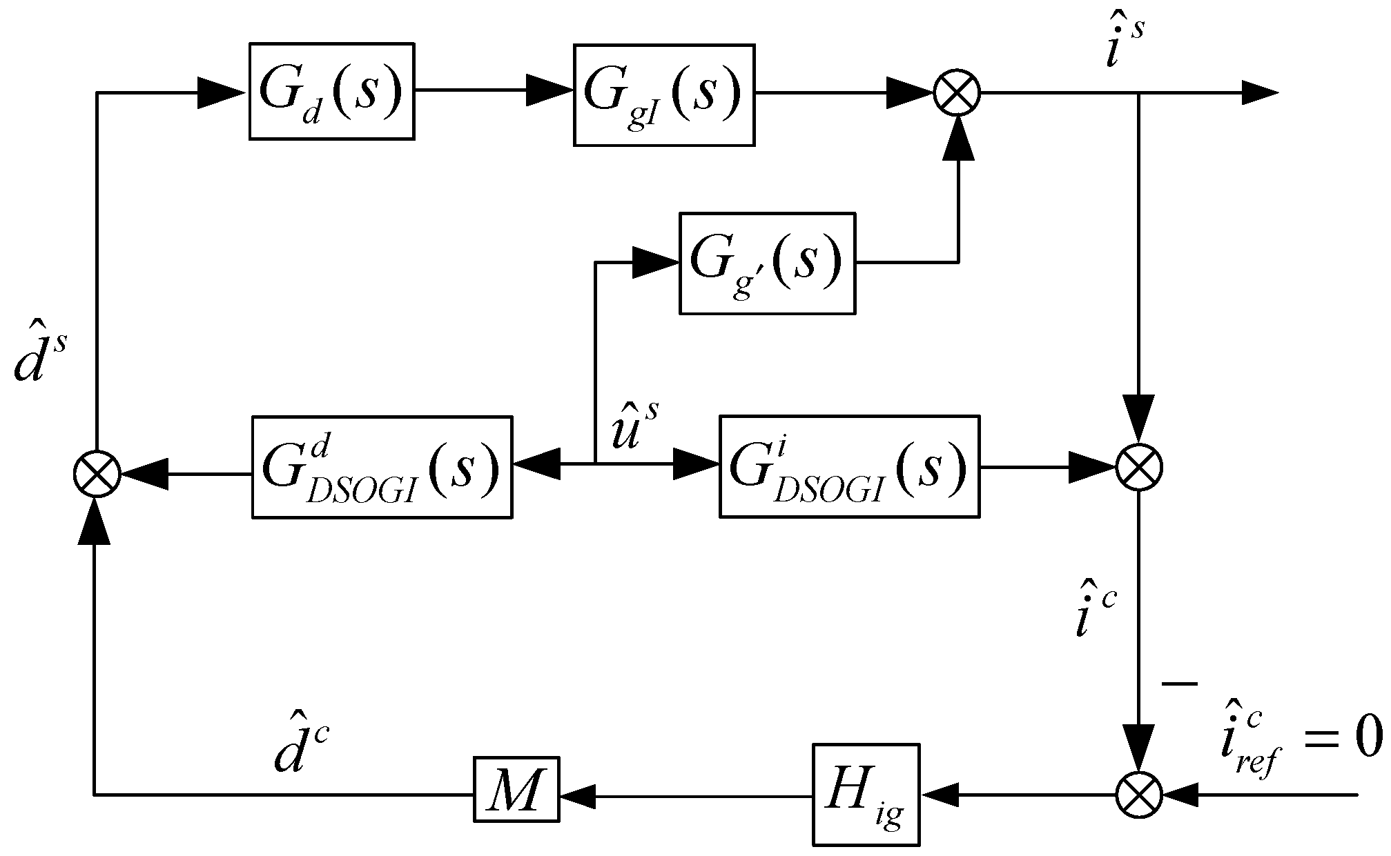
Figure 10 shows the system small signal model considering the PLL. In Figure 10, H_ig is the current loop PI regulator matrix; M is the modulation matrix; G_d is digital delay module, which means sampling switch, one beat delay and zero order retainer link are added to the model. Where Hig = (k_p + k_i/s)*I; M = (1/U_dc)*I; Gd = [(1 − 1.5T_ss)/(1 − 1.5T_ss)]* I; I is 2 × 2 unit matrix.

According to the system small signal control block diagram in Figure 10, the grid-connected inverter output impedance Z_out mathematical model considering the PLL can be derived. As shown in the Equation (26).

$$Z_{out}={[G_{g^{\prime }}+G_{gI}{G}_d(G_{DSOGI}^d-M{H}_{ig}{G}_{DSOGI}^i)]}^{-1}\ast (I+G_{gI}{G}_{d}M{H}_{ig})$$

(26)

2.3.2. Improved Inverter Impedance Model with Feedback Control

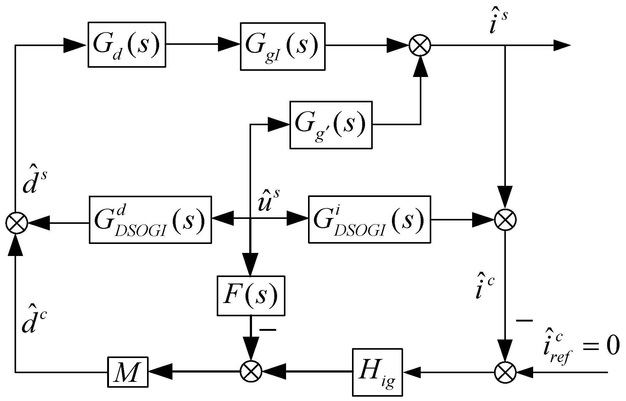
Figure 11 is the improved system small signal model with increased grid terminal voltage compensation. F(s) is the grid voltage feedback matrix expressed as Equation (27).

$$F(s)=\left(\frac{s+400}{s+0.1}\right)I$$

(27)

The improved grid-connected inverter output impedance $Z_{out}^{\prime }$ is shown as Equation (28) deriving from the improved system small-signal model.

$$Z_{out}^{\prime }={[G_{g^{\prime }}+G_{gI}{G}_d({G\prime }_{DSOGI}^d-M{H}_{ig}{G\prime }_{DSOGI}^i+MF(s))]}^{-1}\ast (I+G_{gI}{G}_{d}M{H}_{ig})$$

(28)

where ${G\prime }_{DSOGI}^i$, ${G\prime }_{DSOGI}^d$ represent the transfer function matrix with the improved SOGI-QSG structure of the system voltage to the control loop current and the duty ratio in d-q axis respectively.

3. System Stability Analysis

In order to judge the system stability, the paper adopts the phase margin corresponding to the frequency of intersection between the inverter impedance amplitude-frequency curve and grid impedance amplitude-frequency curve as the judgement standard, as shown in Equation (29).

$$PM={180}^{°}-(\angle Z_g(f_i)-\angle Z_o(f_i))$$

(29)

where Z_g(f_i) and Z_o(f_i) represent the grid input impedance and inverter output impedance of intersection frequency f_i respectively.

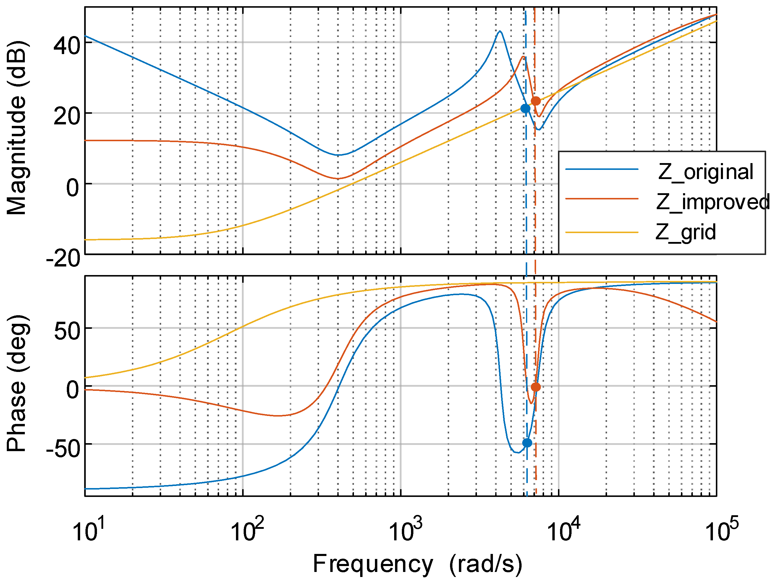
Figure 12 shows the inverter output impedance bode plot front and rear improvement. According to the Figure, the intersection point of amplitude-frequency characteristic curve between the inverter output impedance with feedback control and grid impedance moves to the right compared with the inverter output impedance without control strategy. The phase-frequency characteristic curve of inverter impedance with control strategy is raised compared with the inverter impedance without control strategy. Phase increasing causes the phase margin of the intersection point of amplitude-frequency characteristic between the inverter impedance with feedback control strategy and grid impedance to increase, this is helpful to the system stability in theory.

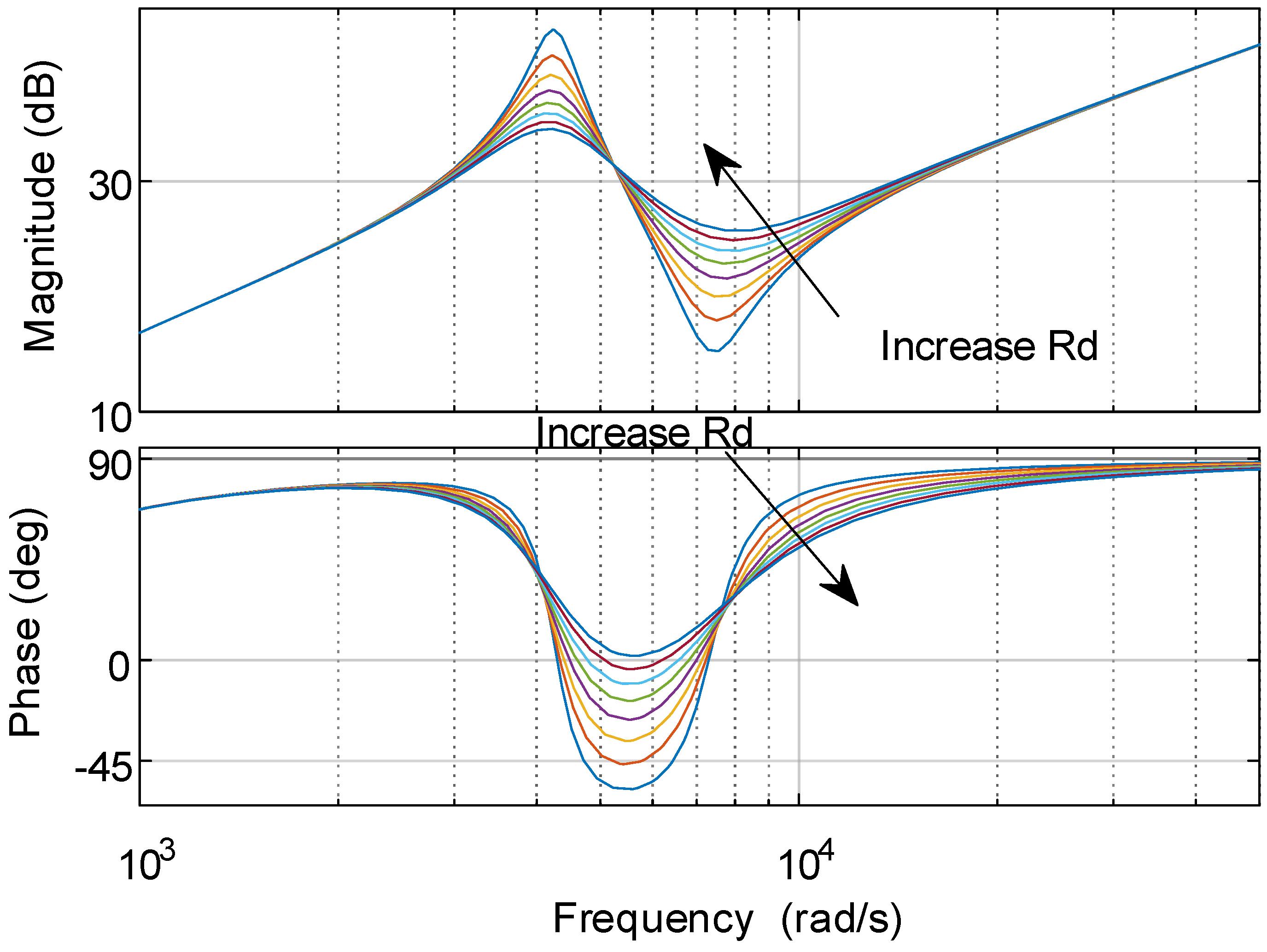
Figure 13 is the Z_dd bode plot with the damping resistance R_d varying from 3 Ω to 10 Ω. In the process of damping resistance increasing, the amplitude-frequency curve intersection point of the inverter impedance and the grid impedance gradually moves to the right and the output impedance phase of the inverter impedance at the corresponding frequency of the intersection point gradually increases. The phase margin increasing gradually is beneficial to the system stability in theory.

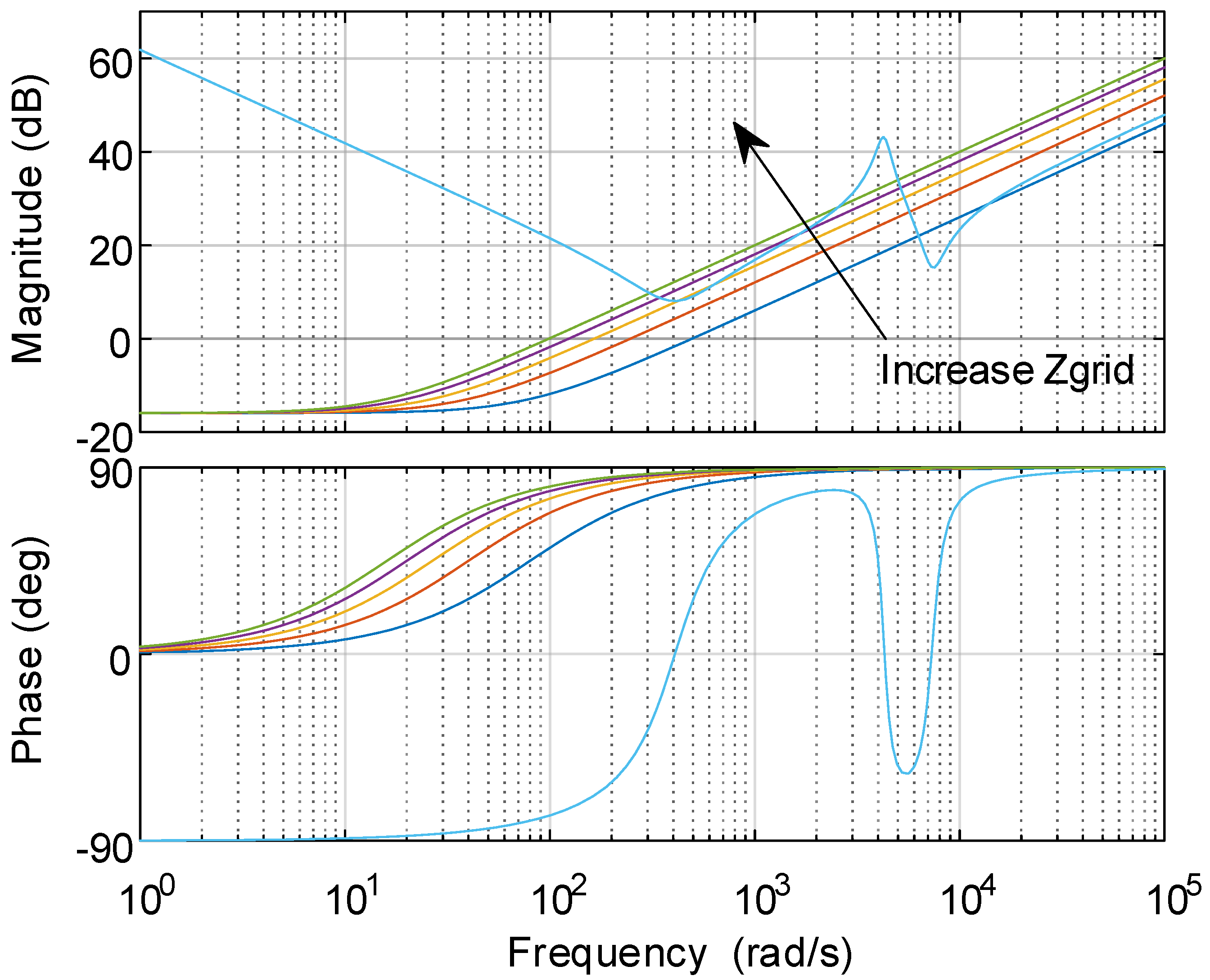
Opposite to the variation trend of the damping resistance R_d. Figure 14 shows the Z_dd bode plot with the grid impedance L_g = 2 mH, r_g = 0.1 Ω and L_g = 5 mH, r_g = 0.1 Ω respectively. As the grid impedance increases, the intersection point of the inverter impedance and the grid impedance amplitude-frequency curve gradually move to the left and the output impedance phase of the inverter impedance at the corresponding frequency of the intersection point gradually decreases. Therefore, the increase of grid impedance is not conducive to the system stability theoretically.

4. Simulation Verification

To verify the correctness of the improvement of SOGI-QSG structure above and the influence of grid impedance on system stability performance. The LCL-type inverter grid-connected system with current loop control is constructed on the Matlab/Simulink simulation platform. The devices used in the simulation are ideal.

Table 1. Main circuit parameters.

Parameter	Value
Set voltage in DC terminal (Udc)	700 V
Effective value of grid voltage (e)	220 V
Machine side inductance (L1)	5 mH
Parasitic resistance of machine side inductor (r1)	0.16 Ω
damping resistance (Rd)	4 Ω
Capacitance (C)	11 μF
Grid side inductance (L2)	2.5 mH
Parasitic resistance of grid side inductor (r2)	0.16 Ω
Grid inductance (Lg)	2 mH
Grid resistance (rg)	0.1 Ω
Switching frequency (fs)	10 kHz

shows the main circuit parameters. Meanwhile,

Table 2. Controller parameters.

PI regulator parameters of current loop

kp = 2.21

ki = 1233

PI regulator parameters of PLL

kp = 0.58

ki = 4.22

shows the PI regulator parameters corresponding to the current loop and PLL respectively. The following passage introduces the simulation validation about two kinds of improved strategies; the PLL characteristics before and after improvement and voltage feedback compensation.

4.1. Phase Locked Loop

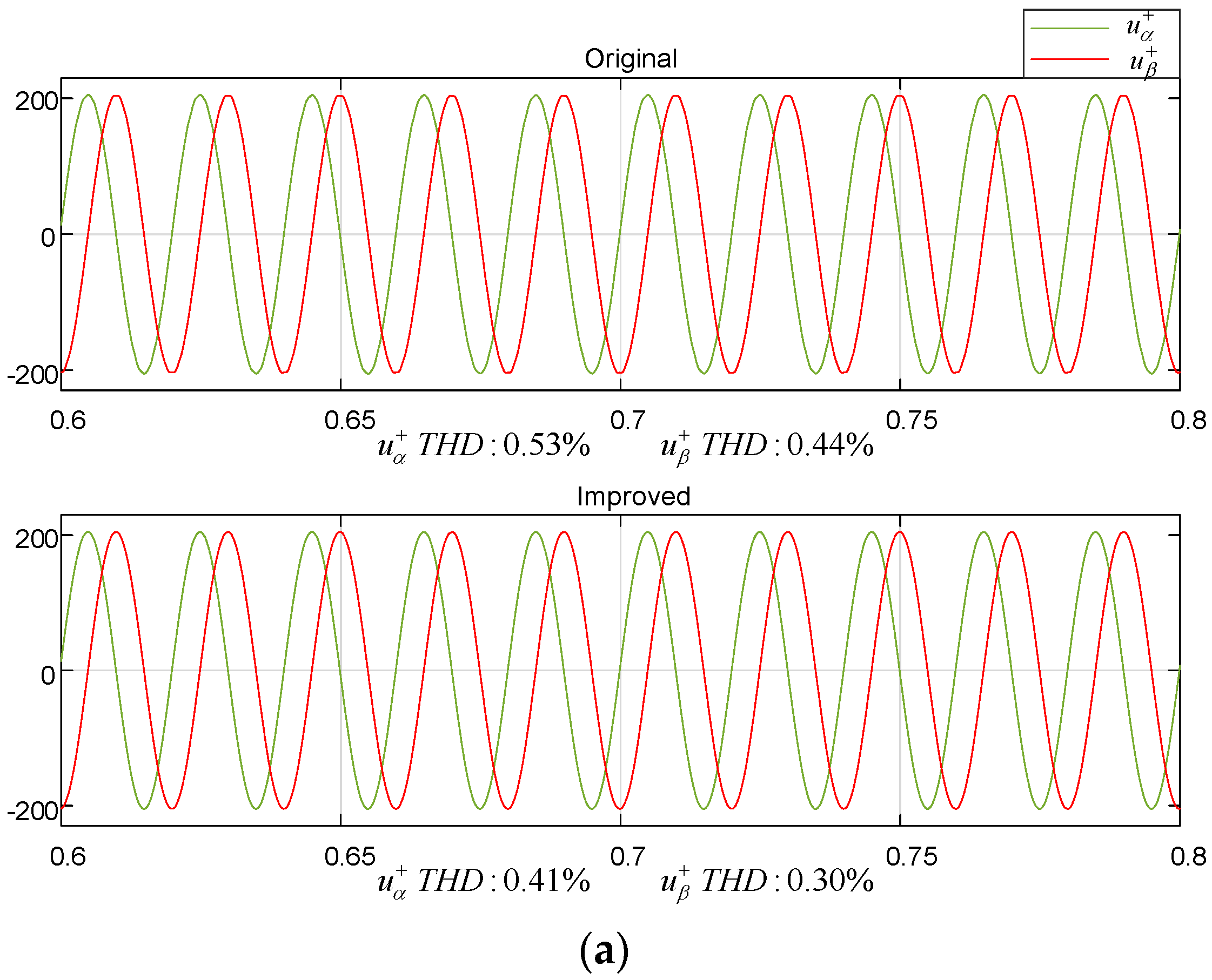
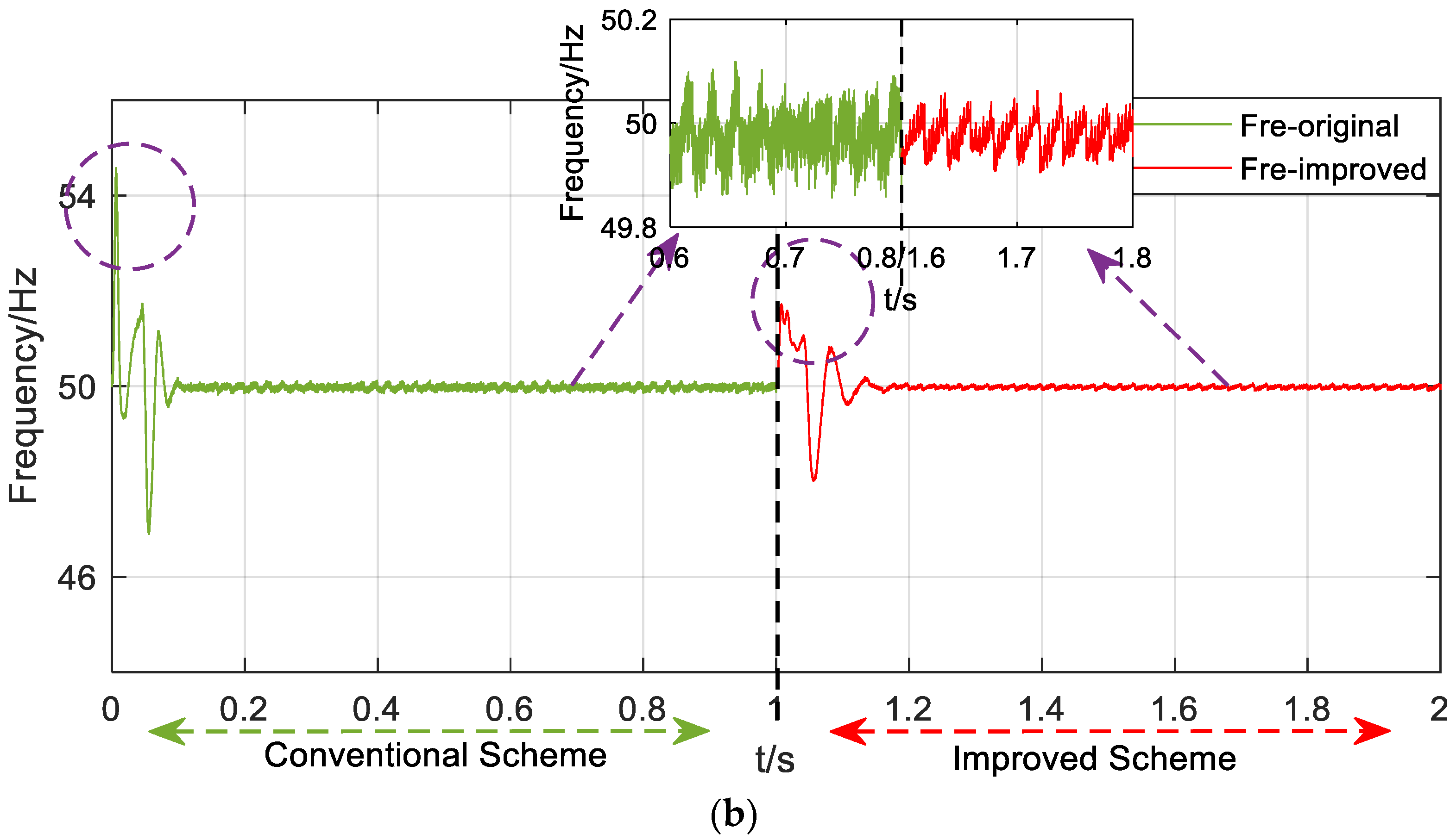
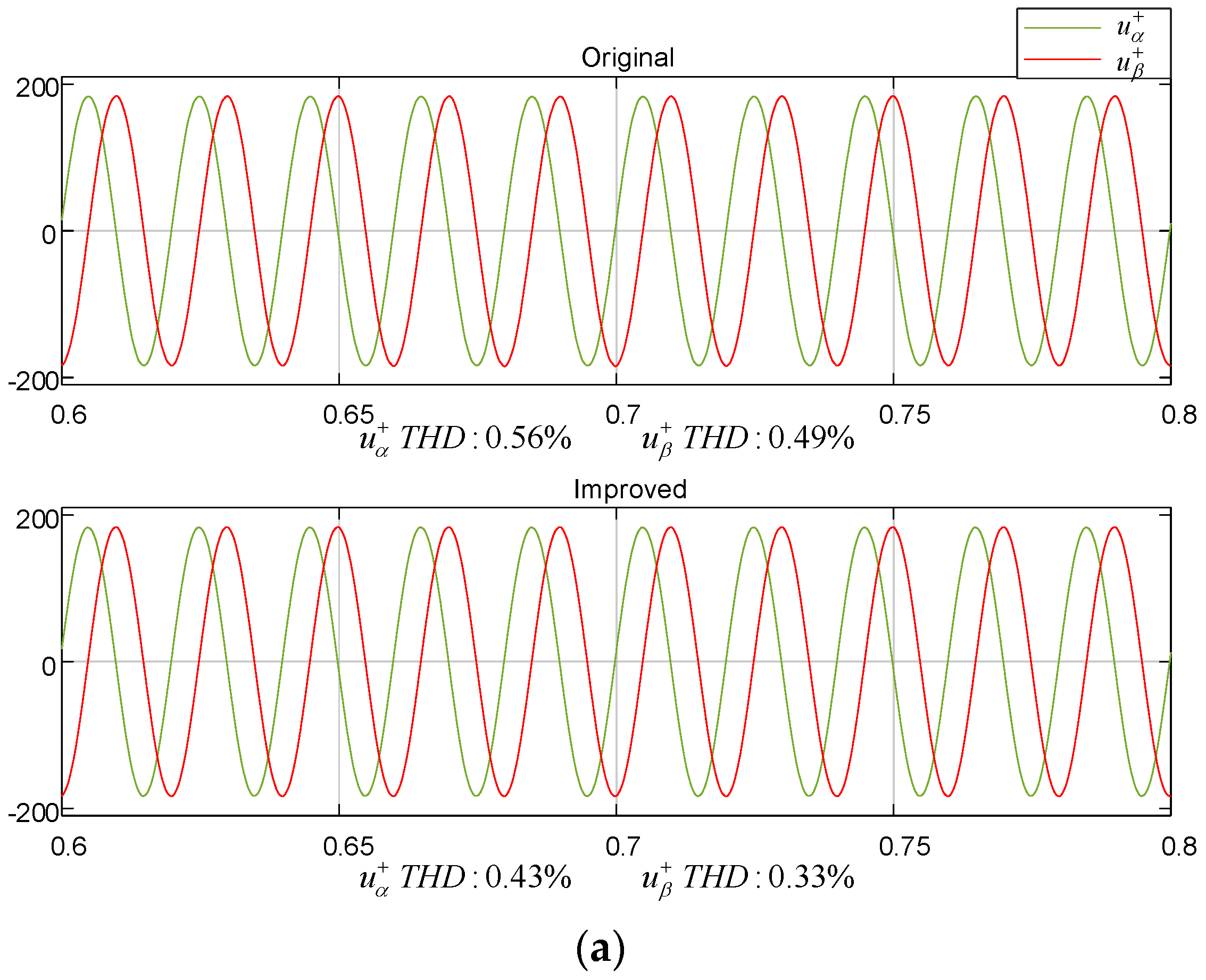
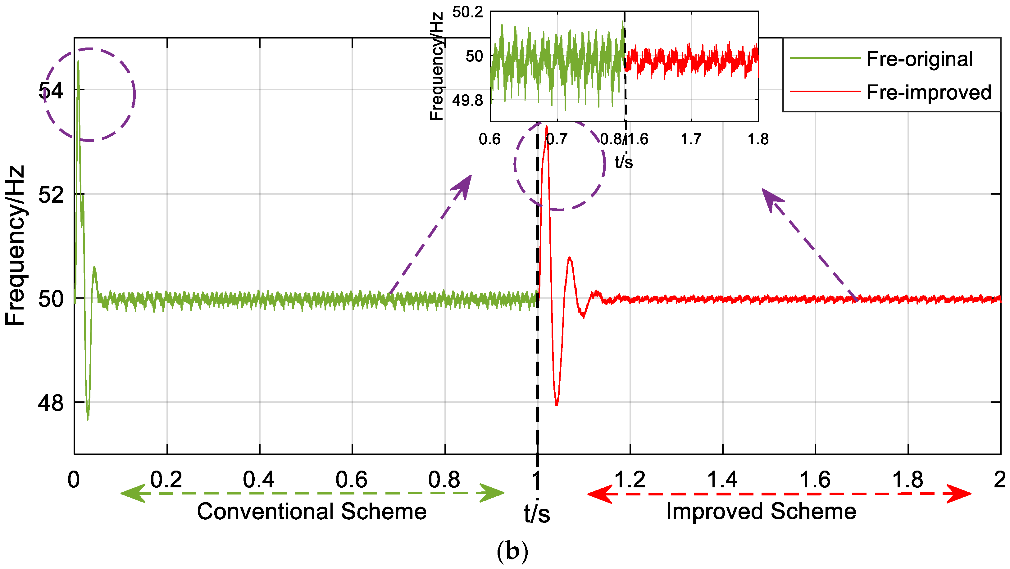
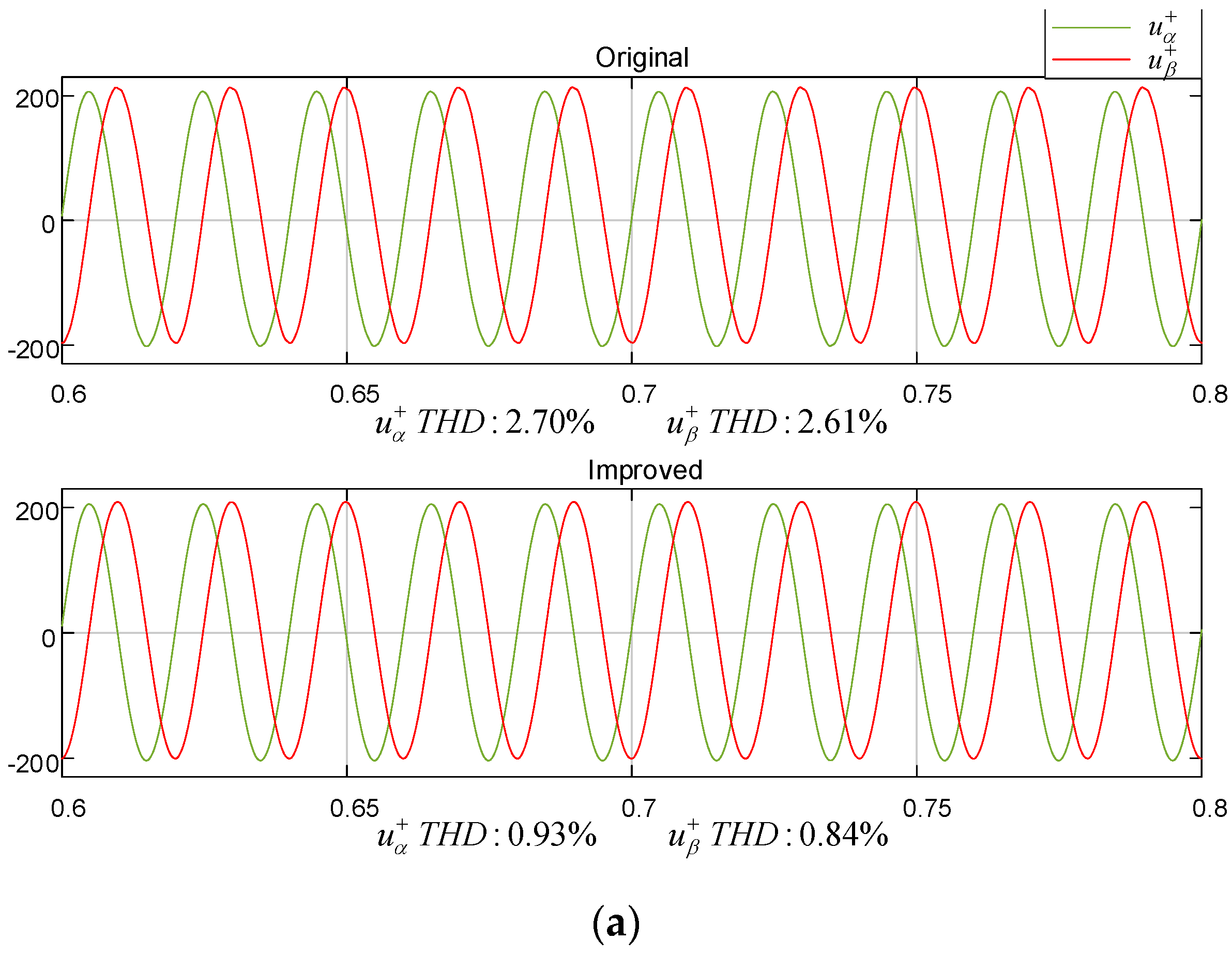
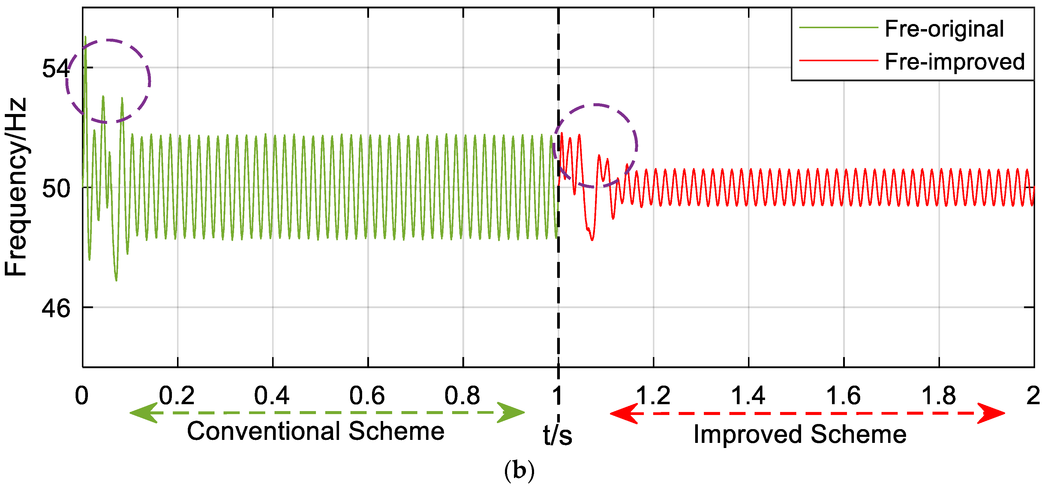
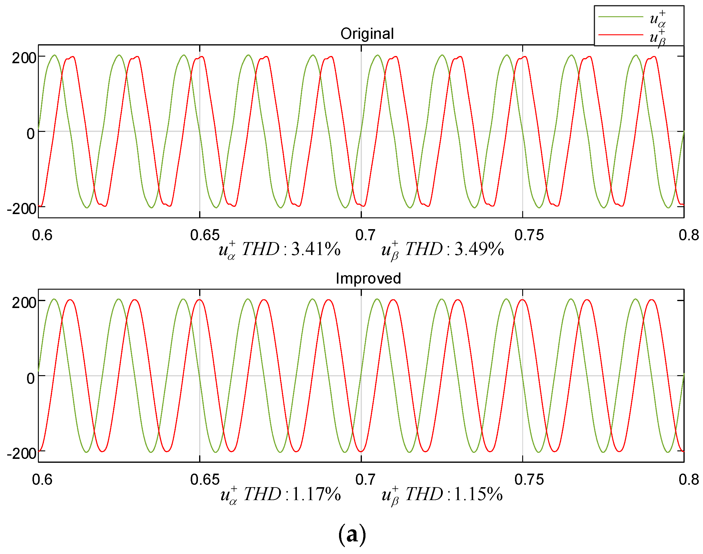
In [8,9], although the control of SRF-PLL is simple, the tracking error is large relatively when the grid voltage contained high harmonic. In [15], Jin et al. adopts the adaptive filter based on SOGI to track error generated by the grid fault, however, it needs to introduce additional devices. Compared with the references, the advantage of the paper is that it does not need to involve additional equipment to obtain accurate phase locking in case of the grid fault. Figure 15, Figure 16, Figure 17 and Figure 18 represent the comparison of the orthogonal signals and frequency waveforms before and after SOGI-QSG structure improvement in different cases. From Figure 15, Figure 16, Figure 17 and Figure 18, Figure (a) shows that the output waveform of positive sequence voltage in the α-β coordinate. Meanwhile, the above is the output waveform of the original SOGI-QSG structure and the below is the waveform of improved structure. Figure (b) is the frequency waveform by integrating q-axis positive sequence voltage through PI regulator. Of which, the left side is frequency waveform of original SOGI-QSG structure by PI regulator, and the right is the waveform of improved structure.

Figure 15 compares the PLL output signals under normal condition which means no grid fault. In the Figure 15a, the total harmonic distortion (THD) of the output positive sequence voltage waveforms of improved SOGI-QSG structure is relatively reduced. In the frequency waveform in Figure 15b it can also be clearly seen that the fluctuation peak value of frequency output decreases, especially in the initial stage of frequency tracking. With the original SOGI-QSG structure, the frequency peak reaches 54.5 Hz within the 0.1 s. While with the improved SOGI-QSG structure, the initial frequency peak only reaches around 52 Hz and the tracking error of PLL on frequency is relatively small in stable state.

Figure 16 shows the output waveform of the SOGI-QSG structure and PLL frequency under the conditions of the grid voltage unbalance. The selected conditions of grid voltage unbalance in the paper are: A phase voltage drops by 30%, while B and C phase voltage remains constant. Compared with the normal operation of grid without fault, the single-phase voltage drop leads to the increment of the distortion rate in positive sequence voltage of PLL output and the enhancement of the frequency fluctuation. Since the voltage amplitude sag is not large, the THD of positive sequence voltage extracted by the PLL is not particularly obvious. However, compared with the original SOGI-QSG structure, the THD of positive sequence voltage extracted by the improved SOGI-QSG structure of PLL decreases, and the peak-peak amplitude of frequency fluctuation also decreases significantly.

Figure 17 shows the output waveform of the SOGI-QSG structure and the PLL frequency when the grid voltage contains a DC component. The selected condition of grid voltage with dc component in the paper is: the A phase voltage is raised by 15%, while B and C phase voltages remains constant. Compared with the aforementioned cases, the THD of positive sequence voltage waveform of SOGI-QSG output increases by 5 times when the grid voltage contains dc component, and the frequency fluctuation is particularly obvious. This also indicates that the dc component included in the grid voltage does cause great interference to the phase-locking. At this point, it is obvious that the THD of positive sequence voltage extracted from improved PLL is reduced about 15% compared with the original SOGI-QSG structure output. The improvement in SOGI-QSG structure is effective to raise the phase locking precision when the dc component included in the grid voltage, at the same time, the frequency fluctuation is also suppressed availably observed from the Figure 17b.

Figure 18 shows the output waveform of the SOGI-QSG structure and the PLL frequency when the grid voltage contains high harmonics. The selected condition of grid voltage with high harmonics in the paper is: three phase voltage contain the 5 harmonic with 110 V amplitude and the 7 harmonic with 66 V amplitude. Compared with the aforementioned three cases, the high-order harmonics included in the grid voltage lead to the obvious distortion of positive sequence voltage with SOGI-QSG structure output. The frequency fluctuation also verifies the phenomenon which indicating that the high-order harmonic of grid voltage is also an important factor resulting to the imprecision of phase locking. By comparing the original SOGI-QSG structure output waveform and frequency output waveform, the reduction of THD in improved SOGI-QSG structure output waveform is simple and clearly illustrates the effectiveness of improvement about SOGI-QSG structure. Meanwhile, it also illustrates that the improved structure is more accurate in tracking phase for the grid voltage with high harmonics.

Table 3. SOGI output THD under different conditions.

	Grid State	Normal	Unbalanced Voltage	DC Components	Harmonic Injection
SOGI Output
Before Improvement (THD)	$u_{\alpha }^{+}$	0.53%	0.56%	2.70%	3.41%
	$u_{\beta }^{+}$	0.44%	0.49%	2.61%	3.49%
After (THD)	$u_{\alpha }^{+}$	0.41%	0.43%	0.93%	1.17%
	$u_{\beta }^{+}$	0.30%	0.33%	0.84%	1.15%

shows the THD of SOGI output waveform under different situations. As shown in Table 3, the improvement in PLL is more effective with the case of DC components and high harmonics than the case with the normal and grid voltages unbalanced conditions. The positive sequence components extracted from the fault input waveforms are more accurate.

4.2. Grid Connected Stability

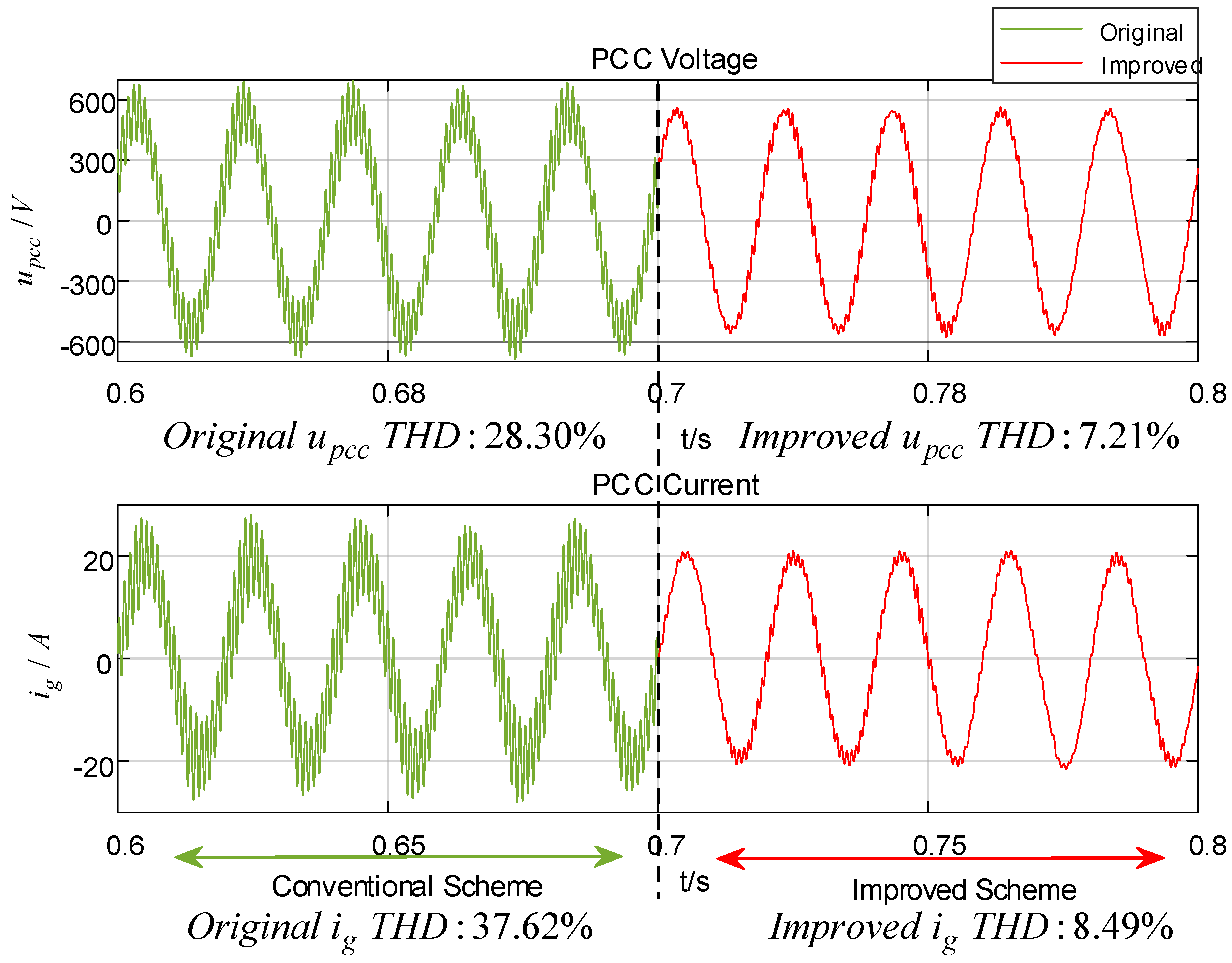
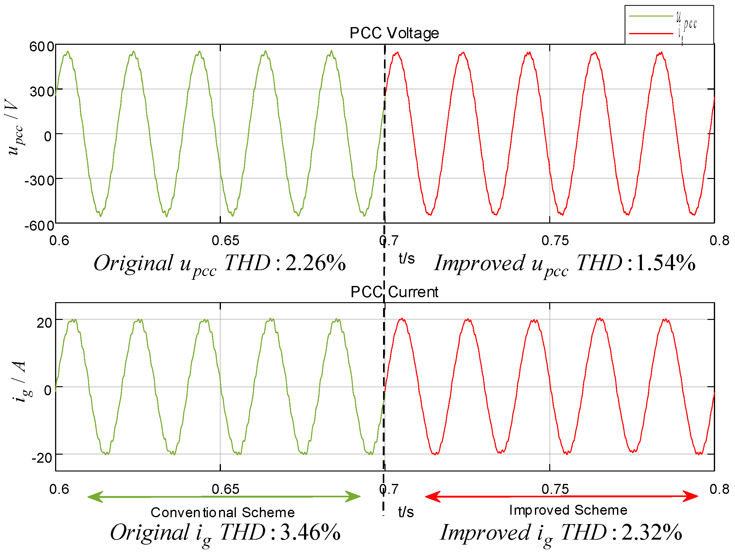
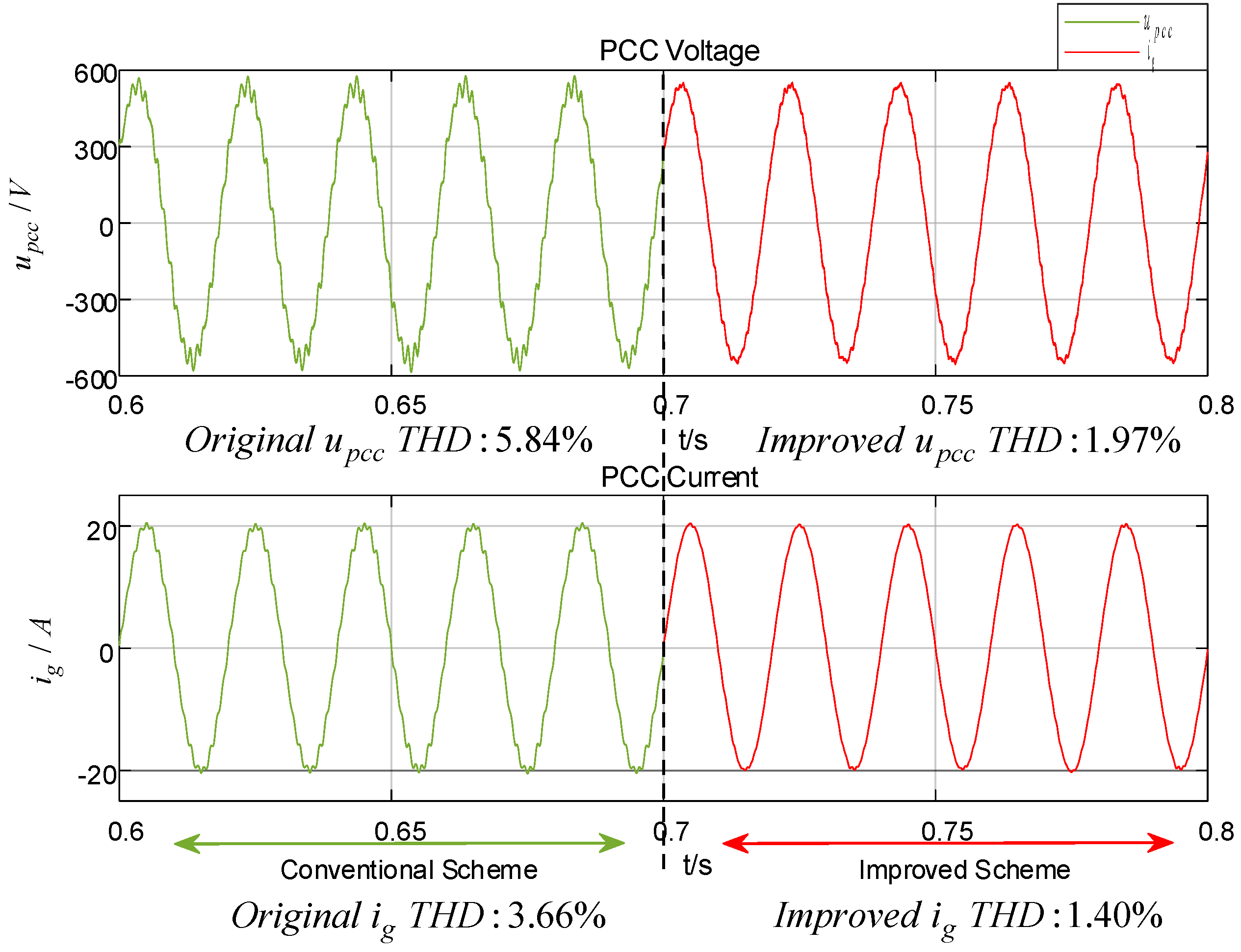
Figure 19 displays the comparison of the grid-connected terminal waveform before and after adding the voltage feedback. When the damping resistance R_d = 1 Ω. Figure 20 and Figure 21 show the comparison of the grid-connected voltage and current waveform before and after adding the voltage feedback when the grid impedance is changed. The above Figure shows the grid-connected voltage waveform and the following Figure shows the grid-connected current waveform. No matter the Figure above or below, the waveform on the left is the output signal without feedback control, while the right signal is the output waveform with feedback control.

The conclusion can be obtained from the system stability analysis in Section 3. The damping resistance R_d is smaller, the phase in frequency intersection between the inverter output impedance and the grid impedance is closer to −90°. The small system phase margin is harm to system stability. In Figure 19, the system oscillates and voltage and current waveform produces distortion when R_d gets smaller. However, the system stability is improved obviously after introducing the voltage feedback, and the waveform distortion rate decays to about 25%.

Figure 20 displays the comparison of the grid-connected voltage and current before and after adding the voltage feedback when the grid impedance parameter is L_g = 2 mH, r_g = 0.1 Ω. As can be seen from the left-right comparison of the grid-connected voltage waveform with or without feedback control strategy, the waveform characteristics have been improved after introducing voltage feedback regardless of grid-connected voltage and current. It can be seen obviously from the THD variation that the voltage and current waveforms THD has been reduced by more than 30% compared with the control strategy without voltage feedback. This is consistent with the analysis of the inverter and grid impedance bode plot in Section 3. The increase of phase margin corresponding to the frequency at the intersection point of the inverter impedance with feedback control and grid impedance amplitude-frequency curve is beneficial to the system being stable theoretically, and the simulation also shows that. The distortion of grid-connected voltage and current are decreased after introducing the feedback control which leads to the output waveform is more stable.

Compared with Figure 20, Figure 21 shows the grid-connected voltage and current comparison before and after adding voltage feedback when the grid impedance parameter is L_g = 5 mH, r_g = 0.1 Ω. As can be seen in Figure 21, the THD of grid-connected voltage and current waveforms increases and the waveforms are distorted with the grid impedance increase compared with the waveforms in the Figure 20. That is to say, the increase of grid impedance is not conducive to the system stability. It is consistent with the aforementioned analysis in theory. The decrease of phase margin corresponding to the frequency at the intersection point between inverter impedance and grid impedance amplitude-frequency curve is more vulnerable to make the system unstable in theory after the grid impedance variation. After introducing the feedback control strategy, the grid-connected voltage and current distortion rate decreases correspondingly and keeps within 2%. The waveform is more stable. Corresponding to the aforementioned analysis in theory, the increase of phase margin corresponding to the frequency at the intersection point between inverter impedance and grid impedance amplitude-frequency curve is more vulnerable to make system stable.

The waveform in Figure 19, Figure 20 and Figure 21 clearly shows that the improved impedance control strategy effectively improves the system stability. It is effective to introduce grid-connected voltage feedback.

5. Conclusions

The paper obtains the improved SOGI-QSG structure by analyzing and optimizing the traditional SOGI-QSG structure against the problem that traditional PLL cannot lock phase precisely in the case of grid fault. The optimized structure improved the filtering ability of the system to high frequency, however, its dynamic response time delay is relatively longer than the original structure, which is not conducive to the system rapid response. Nonetheless, the slight time delay is acceptable compared with the filtering tracking effect of the improved structure. To alleviate the negative influence of the grid impedance variation on the grid-connected system stability, the paper establishes the LCL-type grid-connected inverter impedance model considering the DSOGI-PLL. Based on the impedance analysis method, the paper introduces grid-connected voltage feedback into the current loop to solve the low phase margin problem after analyzing the amplitude-frequency characteristics of the original output impedance. The phase margin at the frequency of intersection is significantly increased and the system is more stable. In the meanwhile, the simulation also illustrates the effectiveness of the proposed strategy, which effectively improves the grid-connected voltage and current distortion rate and enhances the system stability significantly. The paper only analyzes and discusses several special faults of the grid, however there are many other fault phenomena in the grid that are worth researching further.

References

- Mukhopadhyay, S.; Soonee, S.K.; Singh, B.; Sehgal, Y. Opportunities and Problems of Smart Grids with Large Penetration of Renewable Energy-Indian Perspective. In Proceedings of the IEEE Power and Energy Society General Meeting, Vancouver, BC, Canada, 21–25 July 2013. [Google Scholar]
- Bose, B. Power Electronics, Smart Grid, and Renewable Energy Systems. Proc. IEEE 2017, 105, 2011–2018. [Google Scholar] [CrossRef]
- Zeng, M.; Huang, L.; Yan, F.; Jiang, D. Research of the Problems of Renewable Energy Orderly Combined to the Grid in Smart Grid. In Proceedings of the Asia-Pacific Power and Energy Engineering Conference, Chengdu, China, 28–31 March 2010. [Google Scholar]
- Khan, S.; Bletterie, B.; Anta, A.; Gawlik, W. On Small Signal Frequency Stability under Virtual Inertia and the Role of PLLs. Energies 2018, 11, 2372. [Google Scholar] [CrossRef]
- Liu, B.; Zhuo, F.; Zhu, Y.; Yi, H.; Wang, F. A Three-Phase PLL Algorithm Based on Signal Reforming Under Distorted Grid Conditions. IEEE Trans. Power Electron. 2015, 30, 5272–5283. [Google Scholar] [CrossRef]
- Zheng, X.; Xiao, L.; Wang, H.; Liu, S. Grid Frequency Tracking Control Strategy Without PLL for Three-Phase Inverter. In Proceedings of the Energy Conversion Congress and Exposition, Pittsburgh, PA, USA, 14–18 September 2014. [Google Scholar]
- Sawant, R.; Rao, Y. A Discrete-Time Controller for Phase Shift Controlled Load-Resonant Inverter Without PLL. In Proceedings of the IEEE International Conference on Power Electronics, Drives and Energy Systems, Mumbai, India, 16–19 December 2014. [Google Scholar]
- Rasheduzzaman, M.; Khorbotly, S.; Kimball, J. A Modified SRF-PLL for Phase and Frequency Measurement of Single-Phase Systems. In Proceedings of the Energy Conversion Congress and Exposition, Milwaukee, WI, USA, 18–22 September 2016. [Google Scholar]
- Hui, N.; Wang, D.; Li, Y. An Efficient Hybrid Filter-Based Phase-Locked Loop under Adverse Grid Conditions. Energies 2018, 11, 703. [Google Scholar] [CrossRef]
- Nouralinejad, A.; Bagheri, A.; Mardaneh, M.; Malekpour, M. Improving the Decoupled Double SRF PLL for Grid Connected Power Converters. In Proceedings of the Power Electronics, Drive Systems and Technologies Conference, Tehran, Iran, 5–6 February 2014. [Google Scholar]
- Vadlamudi, S.; Jiani, D.; Acosta, M.; Shuyu, C.; Sriram, V.; Tripathi, A. Decoupled DQ-PLL with Positive Sequence Voltage Normalization for Wind Turbine LVRT Control. Energy. In Proceedings of the Power and Transportation Electrification, Singapore, 25–27 October 2016. [Google Scholar]
- Hadjidemetriou, L.; Kyriakides, E.; Blaabjerg, F. A New Hybrid PLL for Interconnecting Renewable Energy Systems to the Grid. IEEE Trans. Ind. Appl. 2013, 49, 2709–2719. [Google Scholar] [CrossRef]
- Rodriguez, P.; Pou, J.; Bergas, J.; Candela, J.; Burgos, R.; Boroyevich, D. Decoupled Double Synchronous Reference Frame PLL for Power Converters Control. IEEE Trans. Power Electron. 2007, 22, 584–592. [Google Scholar] [CrossRef]
- Xie, M.; Wen, H.; Zhu, C.; Yang, Y. DC Offset Rejection Improvement in Single-Phase SOGI-PLL Algorithms: Methods Review and Experimental Evaluation. IEEE Access 2017, 5, 12810–12819. [Google Scholar] [CrossRef]
- Jin, L.; Jiang, M.; Yang, G.; Cheng, Y. Unbalanced Control of Grid-Side Converter Based on DSOGI-PLL. In Proceedings of the IEEE 10th Conference on Industrial Electronics and Applications, Auckland, New Zealand, 15–17 June 2015. [Google Scholar]
- Liu, B.; Wei, Q.; Zou, C.; Duan, S. Stability Analysis of LCL-type Grid-connected Inverter Under Single-loop Inverter-side Current Control with Capacitor Voltage Feedforward. IEEE Trans. Ind. Inf. 2017, 14, 691–702. [Google Scholar] [CrossRef]
- Schiesser, M.; Wasterlain, S.; Marchesoni, M.; Carpita, M. A Simplified Design Strategy for Multi-Resonant Current Control of a Grid-Connected Voltage Source Inverter with an LCL Filter. Energies 2018, 11, 609. [Google Scholar] [CrossRef]
- Xin, Z.; Mattavelli, P.; Yao, W.; Yang, Y.; Blaabjerg, F.; Loh, P. Mitigation of Grid-Current Distortion for LCL-Filtered Voltage-Source Inverter with Inverter-Current Feedback Control. IEEE Trans. Power Electron. 2018, 33, 6248–6261. [Google Scholar] [CrossRef]
- Wen, B.; Boroyevich, D.; Burgos, R.; Mattaveli, P.; Shen, Z. Analysis of D-Q Small-Signal Impedance of Grid-Tied Inverters. IEEE Trans. Power Electron. 2016, 31, 675–687. [Google Scholar] [CrossRef]
- Zeng, Z.; Zhao, R.; Lyu, Z.; Ma, L. Impedance Reshaping of Grid-Tied Inverters to Damp the Series and Parallel Harmonic Resonances of Photovoltaic Systems. Proc. CSEE 2014, 34, 4547–4558. [Google Scholar]
- Chen, X.; Zhang, Y.; Wang, Y. A Study of Dynamic Interaction Between PV Grid-Connected Inverters and Grid Based on the Impedance Analysis Method. Proc. CSEE 2014, 34, 4559–4567. [Google Scholar]
- Wu, H.; Ruan, X.; Yang, D. Research on the Stability Caused by Phase-Locked Loop for LCL-type Grid-Connected Inverter in Weak Grid Condition. Proc. CSEE 2014, 34, 5259–5268. [Google Scholar]
- Sun, J. Impedance-Based Stability Criterion for Grid-Connected Inverters. IEEE Trans. Power Electron. 2011, 26, 3075–3078. [Google Scholar] [CrossRef]
- Liu, Z.; Liu, J.; Hou, X. Output Impedance Modeling and Stability Prediction of Three-Phase Paralleled Inverters With Master–Slave Sharing Scheme Based on Terminal Characteristics of Individual Inverters. IEEE Trans. Power Electron. 2016, 31, 5306–5320. [Google Scholar] [CrossRef]
- Du, Y.; Cui, L.; Yang, X. Impedance-Phase Reshaping of LCL-Filtered Grid-Connected Inverters to Improve the Stability in a Weak Grid. In Proceedings of the IEEE Energy Conversion Congress and Exposition, Cincinnati, OH, USA, 1–5 October 2017. [Google Scholar]
Figure 1.
Equivalent circuit of grid-connection system.
Figure 2.
Grid-connected inverter topology structure.