A GIS-Based Method for Identification of Wide Area Rooftop Suitability for Minimum Size PV Systems Using LiDAR Data and Photogrammetry


Abstract
:
1. Introduction
2. Research Methodology
3. Existing Methods of Rooftop PV Estimation
3.1. Simple Roof Slope and Azimuth Extraction
3.2. Model Driven Methods
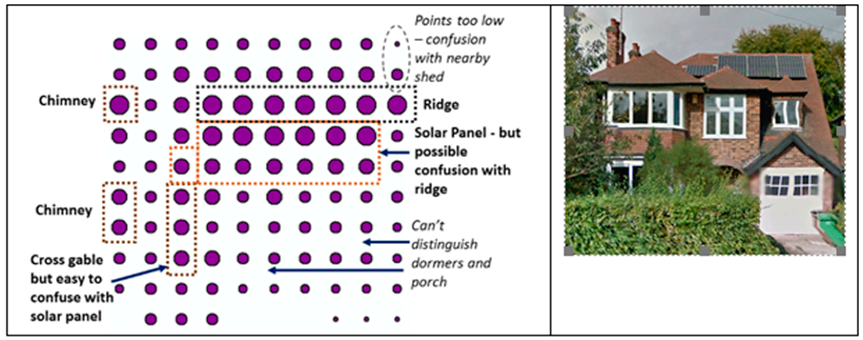
3.3. Histogram Discrimination/Peak Detection
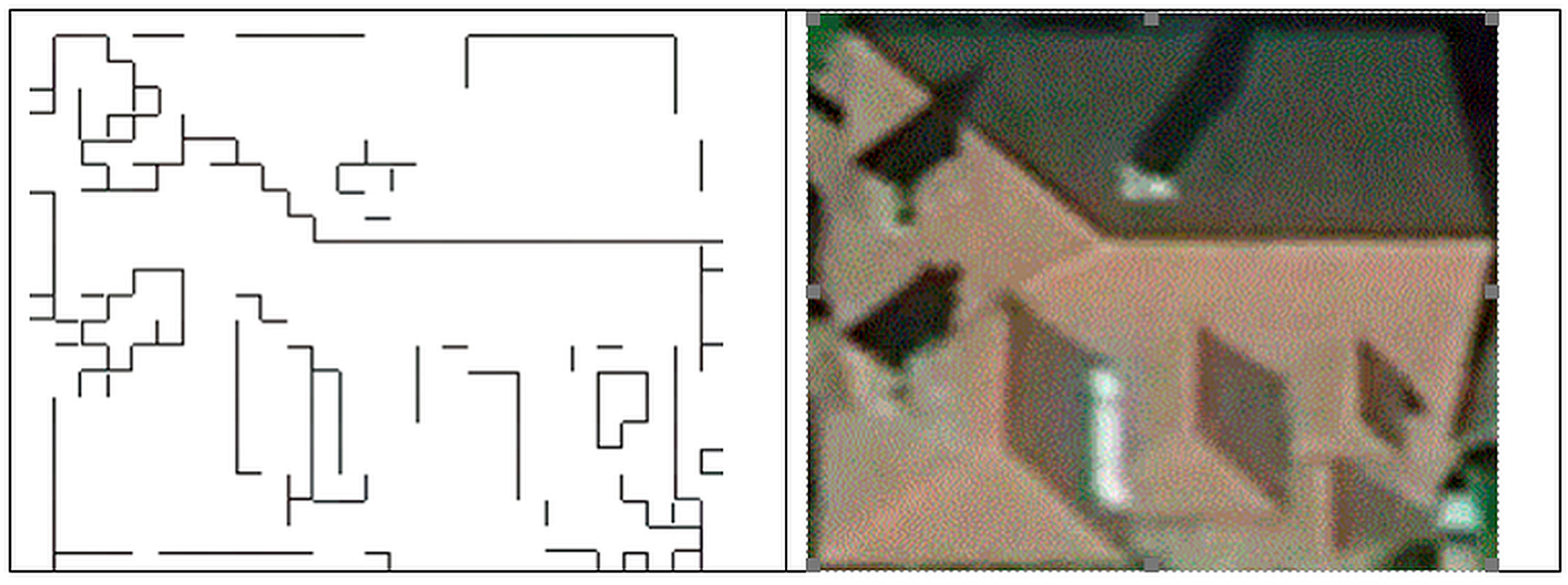
3.4. Edge Detection
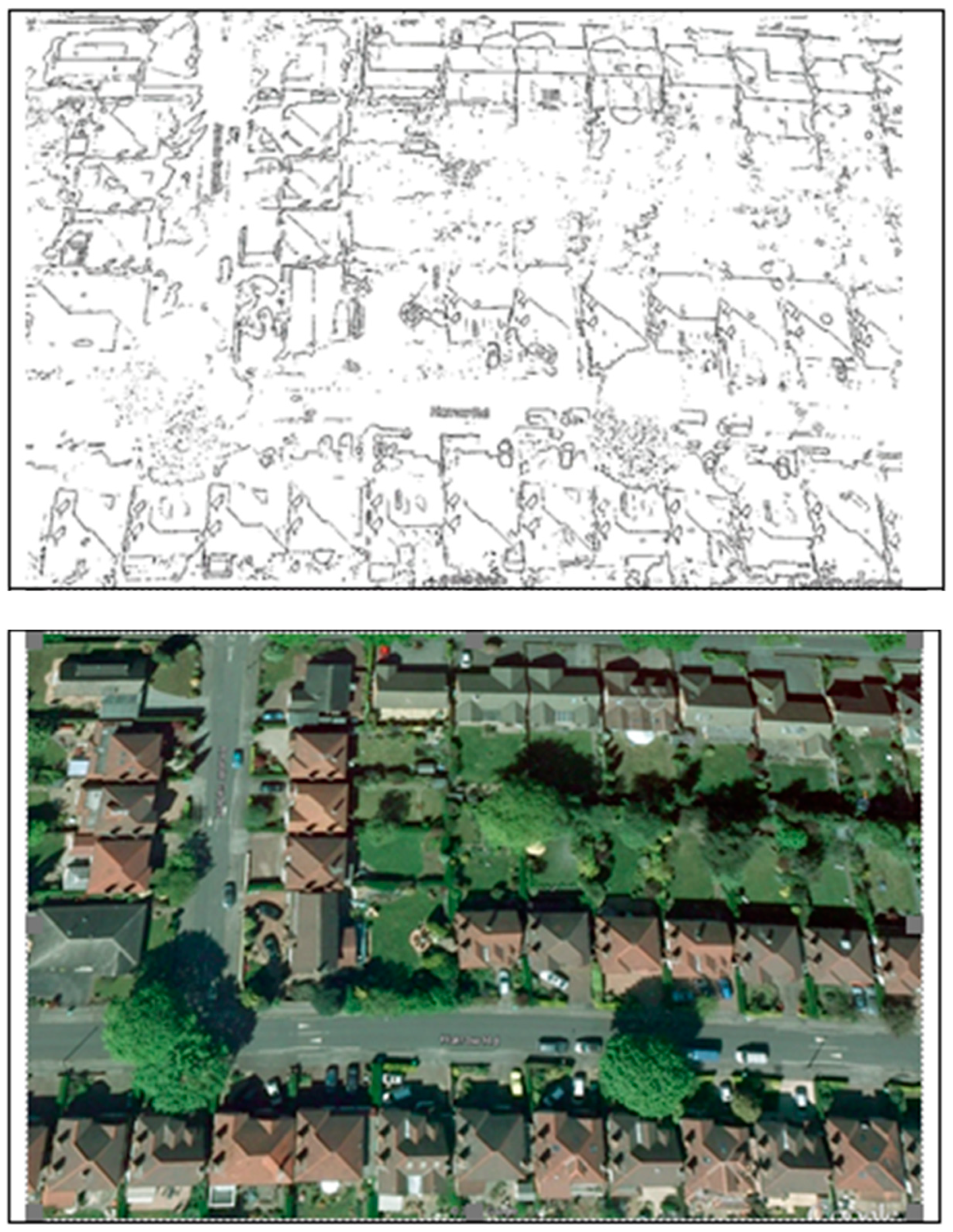
3.5. Edge Detection Using Google Earth
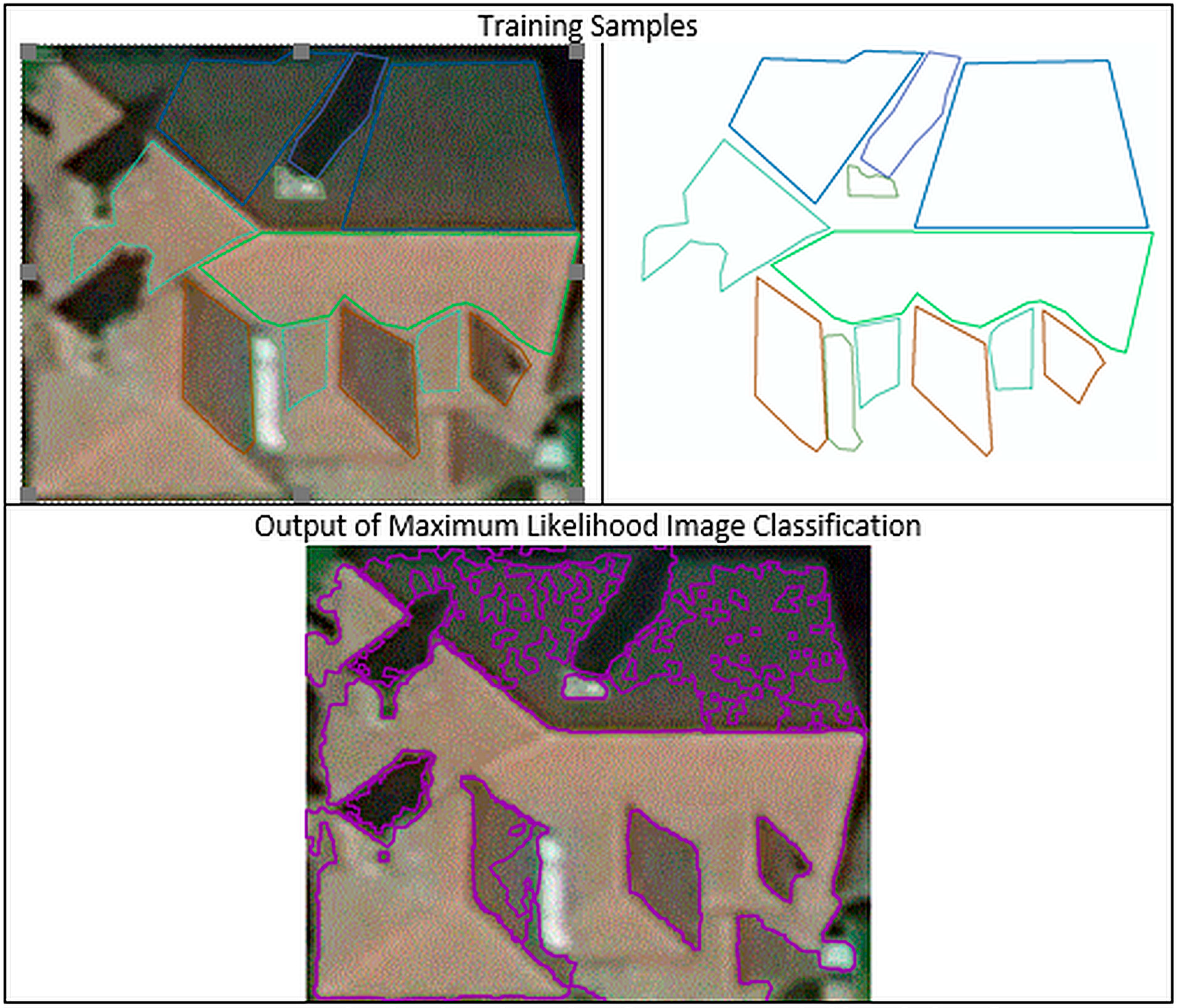
3.6. Image Recognition
- Class probability which employs Bayesian statistics to segment the image.
- Maximum likelihood classification, which also uses Bayes theorem but weights classes if they are more likely to occur.
3.7. Hill Shading with Ambient Occlusion
3.8. Review of Progress
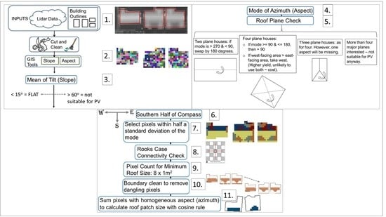
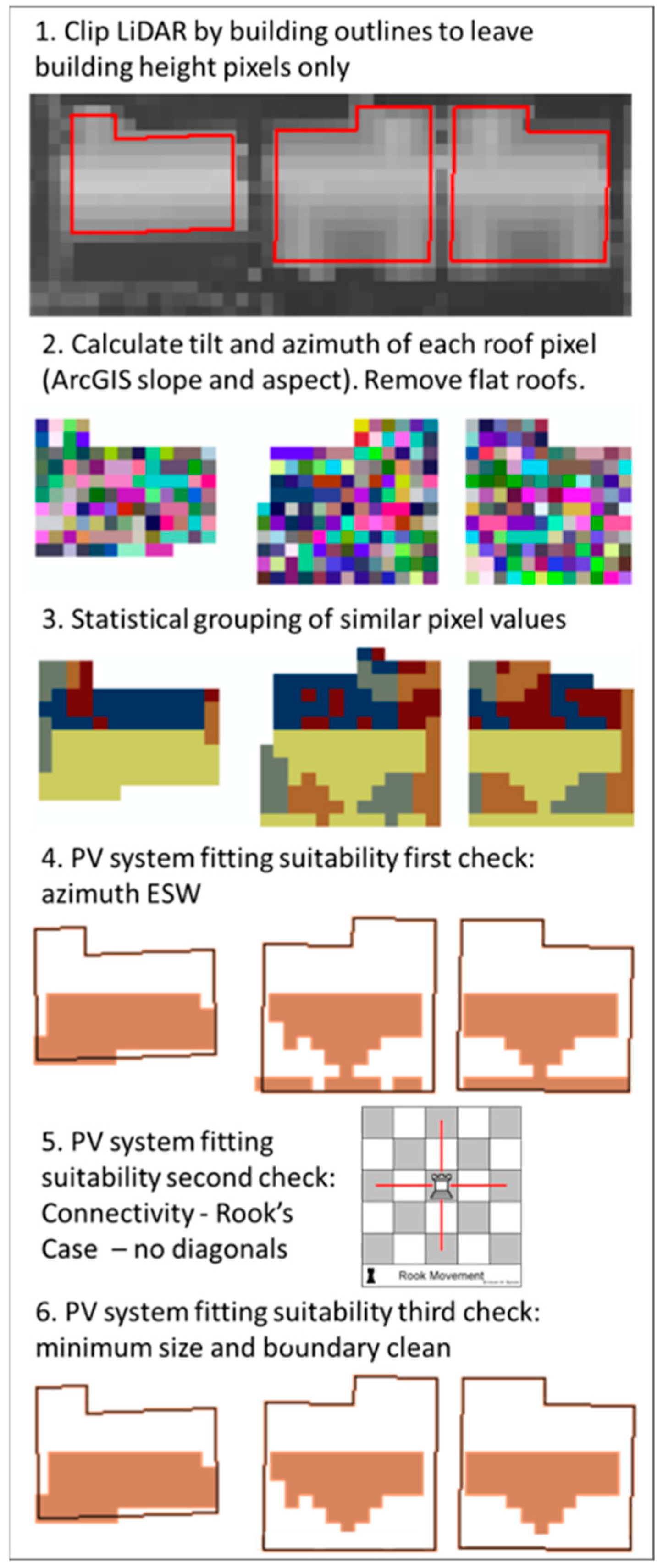
4. New Method
- ArcGIS Slope and Aspect tool are used to calculate the tilt and azimuth of each roof grid square (Figure 9, Step 2).
- The mean tilt of the entire roof is calculated. All main roof patch areas are assigned the same tilt. Accuracy is maximised by taking the entire roof. Roofs with tilts of less than 15° and greater than 60° are excluded. Roofs with a pitch smaller than 15° are not steep enough for accurate azimuth estimations and are categorised as “flat”.
- Determine the mode of azimuth for all grid squares within each building footprint.
- The initial assumption is that all houses have two major aspects. The area is manually checked using Google Earth and extra steps are carried out if more complex building forms are detected:
- Duo pitch roof: Considering due North to be zero degrees, if the mode is between 90° and 270°, add 180° to obtain the southern aspect for PV. In theory an “up and over roof” has two aspect “modes” but due to LiDAR flight paths, reflections, etc. one will predominate. Every pitched roof must have at least two diametric planes. (In contrast to standard peak finding, only one azimuth peak must be found, rather than two.)
- Square four hip roof: If the mode is between 90° and 180°, then add 90°. If the quantity of west-facing grid squares is greater than the amount of east-facing pixels, select the west-facing ones. These receive more insolation and cost will probably prohibit installation on both aspects.
- Three plane houses: Similar to four, but one direction will be missing. If no pixel values are detected in a 10° band when the mode is replaced with the 90° opposite value, this orientation is missing and process is abandoned.
- More than four main roof patches—complex roof formats are not suitable for PV and therefore not covered by this research.
- Select roofs east through south to west (southern cardinal compass directions only).
- Chose grid squares not outside half a standard deviation of the mode (Figure 9, Step 3).
- Carry out a Rook’s Case connectivity check to delete roof patches which are linked by the corners (touch diagonally). PV modules cannot be connected cornerwise (Figure 9, Step 5).
- Apply a minimum 10 pixel filter (10 of 1 × 1 m grid squares) to the selected grid squares to eliminate small areas (Figure 9, Step 6).
- Remove dangling pixels with a boundary clean.
- Roof patch area may be calculated (see Appendix A) if desired, although this is not necessary. It goes beyond the main objective of this approach, which is to select roof planes which meet the three basic technical requirements for PV.
- Equal interval plus or minus 45°.
- Jenks Natural Breaks [61]
- One quarter standard deviation of mode. This gathers almost one sixth of roof data (68% std/4 = 17%).
- One-third standard deviation of mode. This gathers nearly a quarter of roof data (68% std/3 = 23%.
- Half standard deviation of mode. This obtains about one-third of roof data (68% std/2).
5. Results and Validation
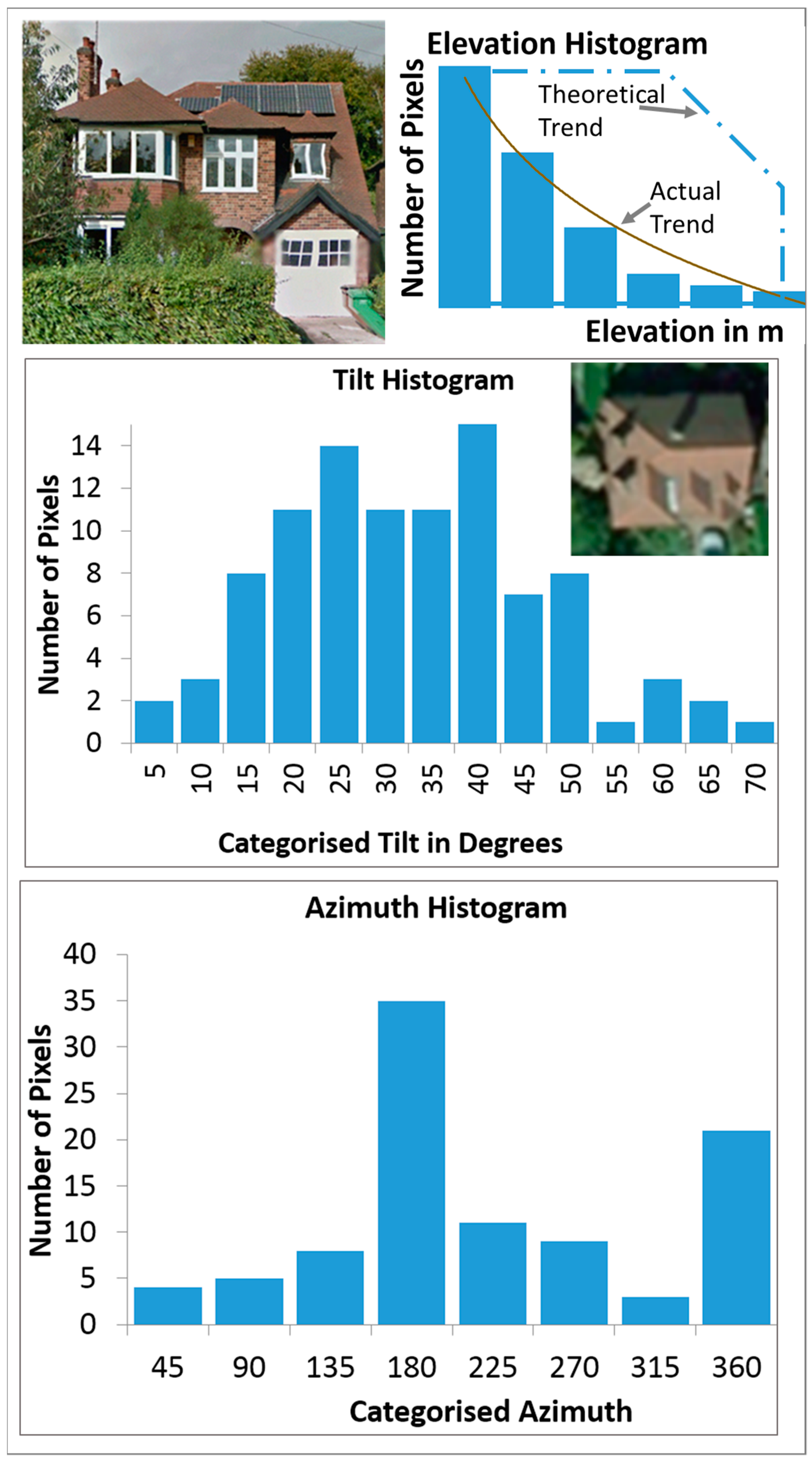
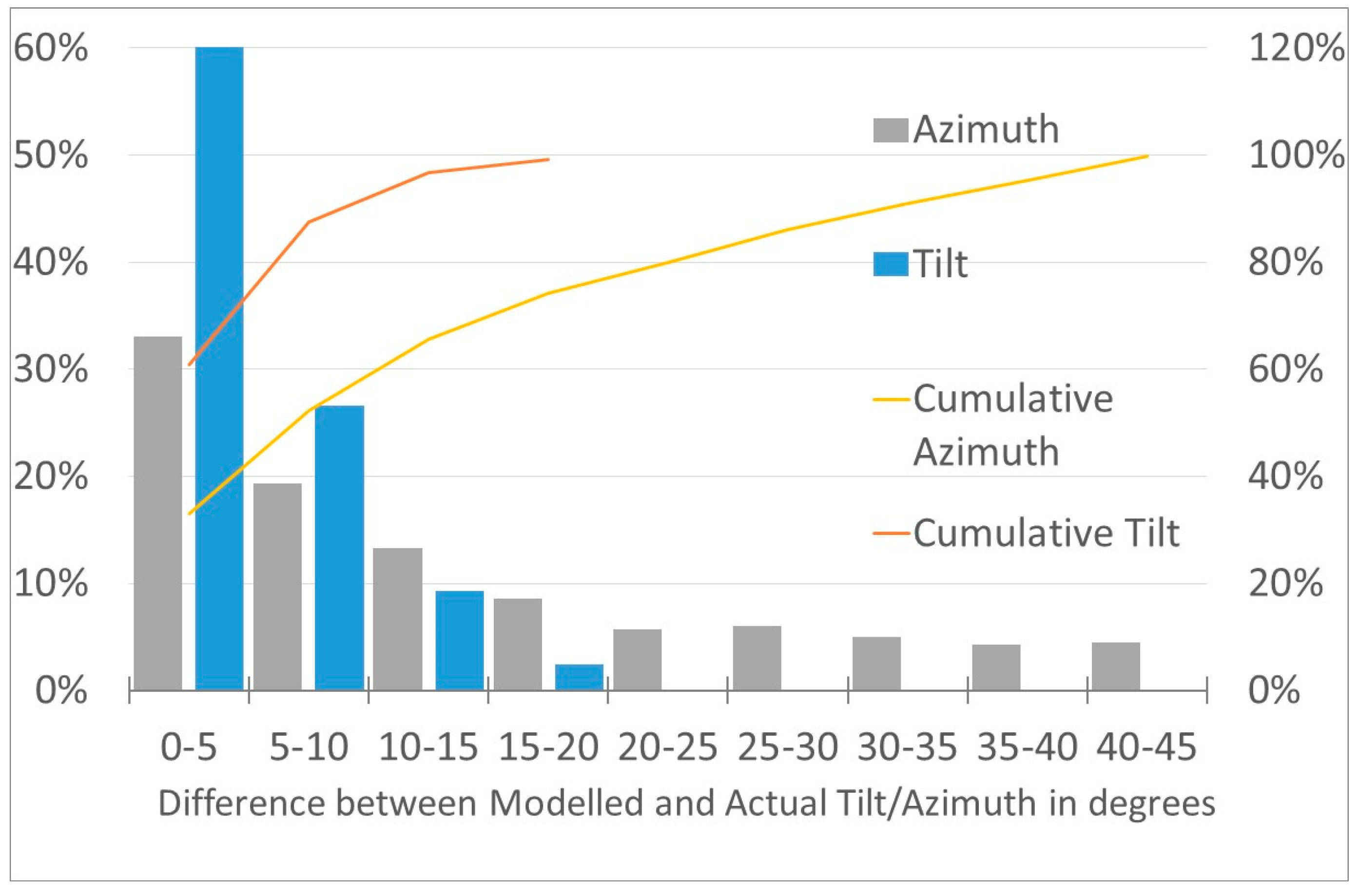
5.1. Tilt
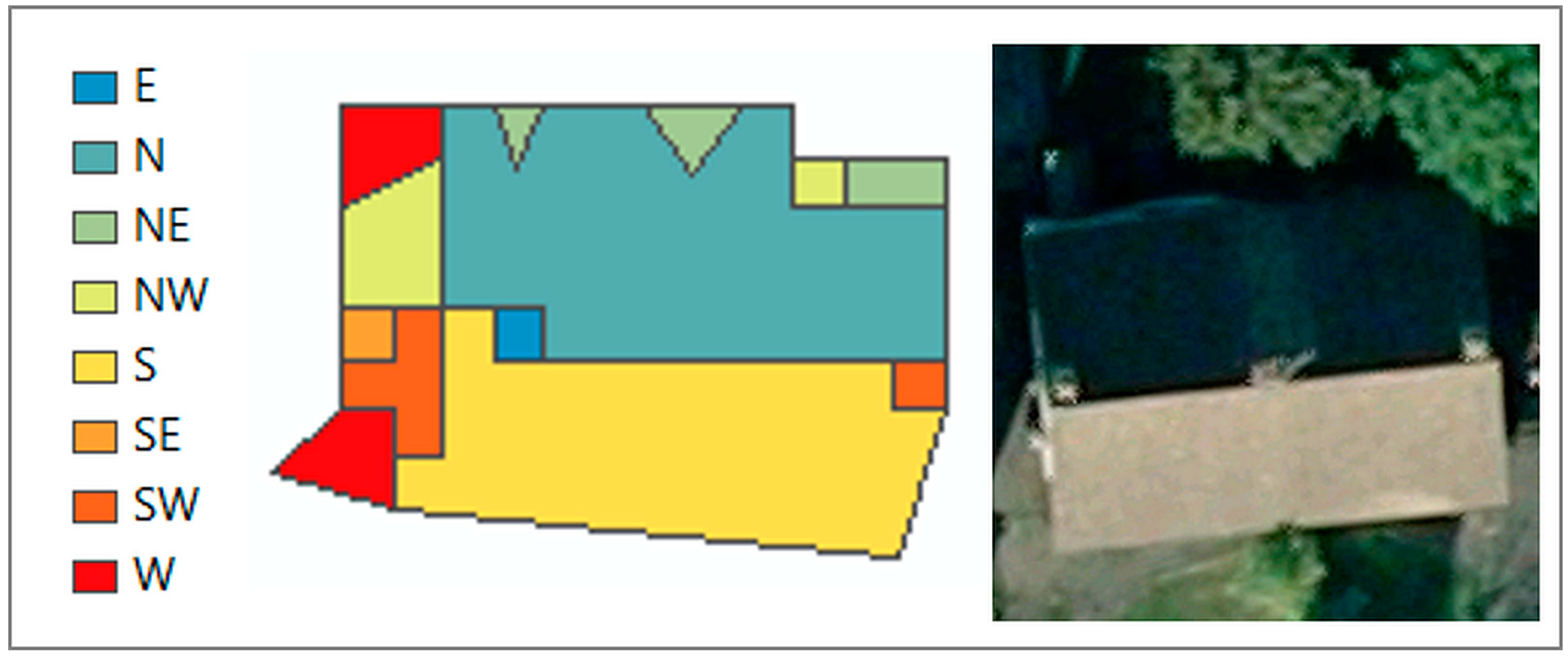
5.2. Azimuth
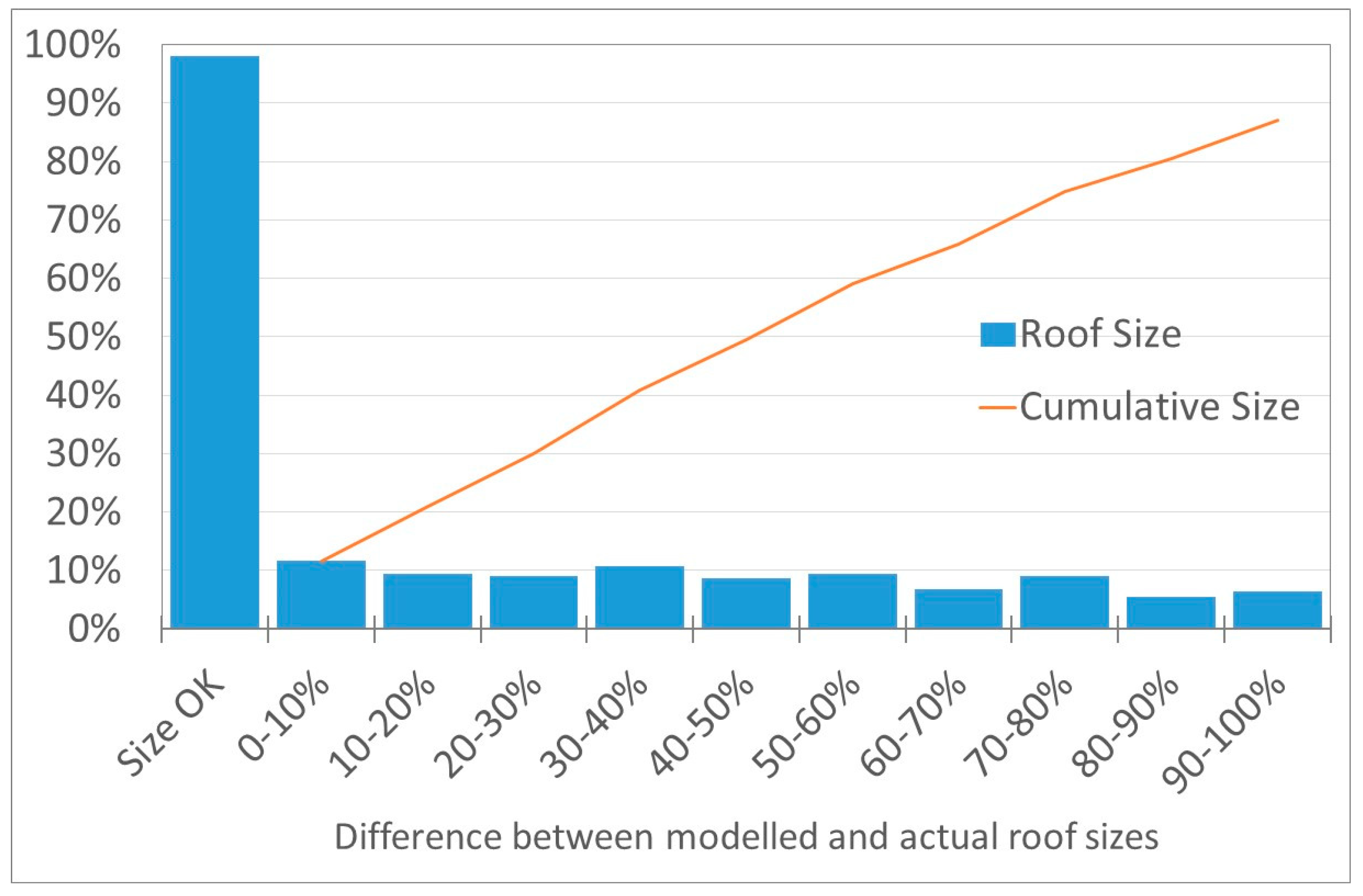
5.3. Roof Patch Area
5.4. Review of Validation
5.5. Context of New Method
6. Summary and Discussion
7. Conclusions
Author Contributions
Funding
Conflicts of Interest
Appendix A
- Preparation: Subtract Environment Agency digital terrain (DTM) LiDAR from the digital surface model (DSM) to obtain building height above ground level. Delete pixels with a lower height than 2 m. This removes rogue values whilst allowing for low eaves.
- Cut out buildings only. Prepared LiDAR DSM-DTM grid and buildings from OS Mastermap Topography layer as inputs: ArcToolbox > Spatial Analyst > Extraction > Extract by Mask.
- Spatial Analyst > Surface > Slope/Aspect. Create integer rasters to enable mode to be computed in the next step.
- Spatial Analyst Tools > Zonal > Zonal Statistics > Mean
- Spatial Analyst Tools > Zonal > Zonal Statistics > Mode
- Mode may be in the north, so carry out some swaps:
- Swap mode raster values by 180:Raster calculator:
- Values between 90 and 270 are alright:Con((“aspectmode” ≤ 270) & (“aspectmode” ≥ 90), “aspectmode”, 0)
- Values between 0 and 90:Con((“aspectmode” ≤ 90) & (“aspectmode” ≥ −1), (“aspectmode” +180), 0)
- Values between 270 and 360:Con((“aspectmode” ≤ 360) & (“aspectmode” ≥ 270), (“aspectmode” −180), 0)
- “PVMode” = “Con1” + “Con2” + “Con3”
- Optionally, switch by 90 east to west for 4-plane houses:Con ((“Con4” ≥ 90) & (“Con4” ≤ 160), (“Con4” +90), “Con4”)
- If the west mode generates a bigger polygon than the east, take that.
- Standard Deviation Bands: Spatial Analyst Tools > Zonal > Zonal Statistics > StdCon ((“intaspect” ≥ “PVMode” − “StdAspect”/2) & (“intaspect” ≤ “PVMode” + “StdAspect”/2), 1, 0)This makes a 1,0 raster of cells half std around the mode.
- Connectivity: ArcToolbox > Spatial Analyst Tools > Generalisation > Region GroupFour neighbours (for edges only, Rooks Case), Cross—exclude zero (“0”).
- Select Large Enough AreasFrom Count because 1 × 1 m pixels. Reclassify as in Table A1 below and discard highest number which is areas not suitable for PV.Table A1. Reclassification of pixel values to enable selection of roof area of at least 8 m2.
Old Values New Values 1–9 NoData 9–19 2 19–30 3 30–44 4 44–63 5 63–96 6 96–175 7 175–302 8 >302 NoData NoData NoData - Clean: Spatial Analyst Tools > Generalisation > Boundary CleanNo sort, run twice.
- Measure Roof Patch with homogeneous aspect (azimuth):Zonal statistics sum points in raster.(Add all the “1”s, not zeroes because “1”s are 1 m squares).
- To calculate a more accurate area allowing for the roof tilt:Slope distance = horizontal distance/cosine(Tilt in degrees)E.g., Slope distance = 21.2 m/cos [32°]

References
- Cîrstea, S.D.; Marti, C.S.; Cîrstea, A.; Dobra, A.C.; Fülöp, M.T. Current Situation and Future Perspectives of the Romanian Renewable Energy. Energies 2018, 11, 3289. [Google Scholar] [CrossRef]
- D’Adamo, I. The Profitability of Residential Photovoltaic Systems. A New Scheme of Subsidies Based on the Price of CO2 in a Developed PV Market. Soc. Sci. 2018, 7, 148. [Google Scholar] [CrossRef]
- Mahmud, M.A.P.; Huda, N.; Farjana, S.H.; Lang, C. Environmental Impacts of Solar-Photovoltaic and Solar-Thermal Systems with Life-Cycle Assessment. Energies 2018, 11, 2346. [Google Scholar] [CrossRef]
- Tsilingiridis, G.; Martinopoulos, G. Thirty years of domestic solar hot water systems use in Greece: Energy and environmental benefits—Future perspectives. Renew. Energy 2010, 35, 490–497. [Google Scholar] [CrossRef]
- Macaulay, J.; Zhou, Z. A Fuzzy Logical-Based Variable Step Size P&O MPPT Algorithm for Photovoltaic System. Energies 2018, 11, 1340. [Google Scholar] [CrossRef]
- PVGIS. Available online: http://re.jrc.ec.europa.eu/pvg_tools/en/tools.html#PVP (accessed on 19 November 2018).
- PVWatts. Available online: https://pvwatts.nrel.gov/ (accessed on 19 November 2018).
- Solargis pvPlanner. Available online: https://solargis.info/pvplanner/#tl=Google:hybrid&bm=satellite (accessed on 19 November 2018).
- PVSol. Available online: https://www.valentin-software.com/en/products/photovoltaics/57/pvsol-premium (accessed on 19 November 2018).
- PVSyst. Available online: http://www.pvsyst.com/en/software (accessed on 19 November 2018).
- European Commission. EU Buildings Database. Policies, Information Services. Available online: https://ec.europa.eu/energy/en/eu-buildings-database (accessed on 4 September 2018).
- Gagnon, P.; Margolis, R.; Melius, J.; Phillips, C.; Elmore, R. Rooftop Solar Photovoltaic Technical Potential in the United States: A Detailed Assessment. 2016. Available online: https://www.nrel.gov/docs/fy16osti/65298.pdf (accessed on 19 November 2018).
- Palmer, D.; Cole, I.; Betts, T.; Gottschalg, R. Assessment of potential for photovoltaic roof installations by extraction of roof tilt from light detection and ranging data and aggregation to census geography. IET Renew. Power Gener. 2016, 10, 467–473. [Google Scholar] [CrossRef] [Green Version]
- Palmer, D.; Cole, I.R.; Goss, B.; Betts, T.R.; Gottschalg, R. Detection of roof shading for PV based on LiDAR data using a multi-modal approach. In Proceedings of the 31st European Photovoltaic Solar Energy Conference and Exhibition, Hamburg, Germany, 14–18 September 2015; pp. 1753–1759. Available online: https://www.eupvsec-proceedings.com/proceedings?paper=32667 (accessed on 19 November 2018).
- Goss, B.; Cole, I.R.; Koubli, E.; Palmer, D.; Betts, T.R.; Gottschalg, R. Modelling and prediction of PV module energy yield. In The Performance of Photovoltaic (PV) System: Modelling, Measurement and Assessment; Pearsall, N., Ed.; Elsevier Ltd.: Amsterdam, The Netherlands, 2016; pp. 103–134. [Google Scholar]
- Nottingham City Homes; (Nottingham, UK). Personal communication, 2016.
- Zsiborács, H.; Bai, A.; Popp, J.; Gabnai, Z.; Pály, B.; Farkas, I.; Baranyai, N.H.; Veszelka, M.; Zentkó, L.; Pintér, G. Change of Real and Simulated Energy Production of Certain Photovoltaic Technologies in Relation to Orientation, Tilt Angle and Dual-Axis Sun-Tracking. A Case Study in Hungary. Sustainability 2018, 10, 1394. [Google Scholar] [CrossRef]
- Vu, H.N.; Shin, S. Flat Concentrator Photovoltaic System with Lateral Displacement Tracking for Residential Rooftops. Energies 2018, 11, 114. [Google Scholar] [CrossRef]
- Renno, C. Experimental and Theoretical Analysis of a Linear Focus CPV/T System for Cogeneration Purposes. Energies 2018, 11, 2960. [Google Scholar] [CrossRef]
- DBEIS. Solar Photovoltaics Deployment. National Statistics. Available online: https://www.gov.uk/government/statistics/solar-photovoltaics-deployment (accessed on 4 September 2018).
- Masson, G.; Kaizuka, I. Trends 2017 in Photovoltaic Applications. Report IEA PVPS T1-32:2017. Survey Report of Selected IEA Countries between 1992 and 2016, Edition 22. Available online: https://www.researchgate.net/publication/324728347_TRENDS_2017_IN_PHOTOVOLTAIC_APPLICATIONS (accessed on 19 November 2018).
- Riksdienst voor Ondernemend Nederland. International Positioning of the Dutch PV Sector. Final Report for Publication. 2014. Available online: https://www.rvo.nl/sites/default/files/2014/08/International%20positioning%20of%20the%20Dutch%20PV%20sector%20final.pdf (accessed on 19 November 2018).
- Liu, Y. Solar PV in China Looks Promising for 2018. Renewable Energy World, 2018. Available online: https://www.renewableenergyworld.com/articles/2018/03/solar-pv-in-china-looks-promising-for-2018.html (accessed on 19 November 2018).
- Hafez, A.Z.; Soliman, A.; El-Metwally, K.A.; Ismail, I.M. Tilt and azimuth angles in solar energy applications—A review. Renew. Sustain. Energy Rev. 2017, 77, 147–168. [Google Scholar] [CrossRef]
- Hartner, M.; Ortner, A.; Heisl, A.; Haas, R. East to west—The optimal tilt angle and orientation of photovoltaic panels from an electricity system perspective. Appl. Energy 2015, 160, 94–107. [Google Scholar] [CrossRef]
- Zsiborács, H.; Baranyai, N.H.; Vincze, A.; Háber, I.; Pintér, G. Economic and Technical Aspects of Flexible Storage Photovoltaic Systems in Europe. Energies 2018, 11, 1445. [Google Scholar] [CrossRef]
- Marinić-Kragić, I.; Nižetić, S.; Grubišić-Čabo, F.; Papadopoulos, A.M. Analysis of flow separation effect in the case of the free-standing photovoltaic panel exposed to various operating conditions. J. Clean. Prod. 2018, 174, 53–64. [Google Scholar] [CrossRef]
- Davies, J. A Guide to Roof Construction—Part 1. Available online: Great-home.co.uk/a-guide-to-roof-construction/ (accessed on 19 November 2018).
- Vaughn, T.G.I. What Is the Typical Roof Pitch on a Mediterranean Style Home? Available online: https://www.houzz.com/discussions/4046877/what-is-the-typical-roof-pitch-on-a-mediterranean-style-home (accessed on 6 September 2018).
- Melius, J.; Margolis, R.; Ong, S. Estimating Rooftop Suitability for PV: A Review of Methods, Patents, and Validation Techniques. 2013. Available online: https://digital.library.unt.edu/ark:/67531/metadc866924/m2/1/high_res_d/1117057.pdf (accessed on 19 November 2018).[Green Version]
- Hong, T.; Lee, M.; Koo, C.; Jeong, K.; Kim, J. Development of a Method for estimating the Rooftop Solar Photovoltaic (PV) Potential by Analyzing the Available Rooftop Area Using Hillshade Analysis. Appl. Energy 2017, 194, 320–332. [Google Scholar] [CrossRef]
- Boz, B.M.; Calvert, K.; Brownson, J.R.S. An automated model for rooftop PV systems assessment in ArcGIS using LIDAR. AIMS Energy 2015, 3, 401–420. [Google Scholar]
- Campana, P.E.; Quan, S.J.; Robbio, F.I.; Lundblad, A.; Zhang, Y.; Ma, T.; Karlsson, B.; Yan, J. Optimization of a residential district with special consideration on energy and water reliability. Appl. Energy 2017, 194, 751–764. [Google Scholar] [CrossRef]
- Theodoridou, I.; Karteris, M.; Mallinis, G.; Papadopoulos, A.M.; Hegger, M. Assessment of retrofitting measures and solar systems’ potential in urban areas using Geographical Information Systems: Application to a Mediterranean city. Renew. Sustain. Energy Rev. 2012, 16, 6239–6261. [Google Scholar] [CrossRef]
- Ordonez, J.; Jadraque, E.; Alegre, J.; Martinez, G. Analysis of the Photovoltaic Solar Energy Capacity of Residential Rooftops in Andalusia (Spain). Renew. Sustain. Energy Rev. 2010, 14, 2122–2130. [Google Scholar] [CrossRef]
- Environment Agency. Survey Open Data. Available online: http://environment.data.gov.uk/ds/survey/#/survey (accessed on 11 January 2018).
- Google Earth. Pr9 V7.3.2.5491. Digital Globe: Nottingham, UK, 2012; Available online: http://www.google.com/earth/download/ge/ (accessed on 19 November 2018).
- Laporte, J. What Size Solar Panel Do I Need For My Home?—The Eco Expert. Available online: https://www.theecoexperts.co.uk/solar-panels/what-size-do-i-need (accessed on 13 November 2018).
- Ordnance Survey. OS MasterMap Topography Layer. 2014. Available online: https://www.ordnancesurvey.co.uk/business-and-government/products/topography-layer.html (accessed on 10 June 2017).
- Burrough, P.A.; McDonell, R.A. Principles of Geographical Information Systems; Oxford University Press: New York, NY, USA, 1998. [Google Scholar]
- Jacques, D.A.; Gooding, J.; Giesekam, J.J.; Tomlin, A.S.; Crook, R. Methodology for the assessment of PV capacity over a city region using low-resolution LiDAR data and application to the City of Leeds (UK). Appl. Energy 2014, 124, 28–34. [Google Scholar] [CrossRef] [Green Version]
- Wikipedia. List of Roof Shapes. 2018. Available online: https://en.wikipedia.org/wiki/List_of_roof_shapes (accessed on 19 November 2018).
- Ballard, S.; Dibb, M.; Facey, P.; Hunter, B.; Johnstone, C.; Stott, R. Geograph Britain and Ireland. 2005. Available online: http://www.geograph.org.uk (accessed on 11 January 2018).
- Stilla, U.; Jurkiewicz, K. Automatic reconstruction of roofs from maps and elevation data. Int. Arch. Photogramm. Remote Sens. 1999, 32. Available online: https://www.pf.bgu.tum.de/pub/1999/stilla_jurkiewicz_isprs99_pap.pdf (accessed on 19 November 2018).
- Lukač, N.; Žlaus, D.; Seme, S.; Žalik, B.; Štumberger, G. Rating of roofs’ surfaces regarding their solar potential and suitability for PV systems, based on LiDAR data. Appl. Energy 2013, 102, 803–812. [Google Scholar] [CrossRef]
- Demir, N.; Baltsavias, E. Automated Modeling of 3D Building Roofs Using Image and Lidar Data. ISPRS Ann. Photogramm. Remote Sens. Spat. Inf. Sci. 2012, 25, 35–40. [Google Scholar] [CrossRef]
- Tarsha-Kurdi, F.; Landes, T.; Grussenmeyer, P.; Koehl, M. Model-Driven and Data-Driven Approaches Using Lidar Data: Analysis and Comparison. PIA07—Photogrammetric Image Analysis 2007. Available online: https://halshs.archives-ouvertes.fr/file/index/docid/264846/filename/Tarsha_TL_PG_MK_PIA_07.pdf (accessed on 19 November 2018).
- Canny, J. A computational approach to edge detection. IEEE Trans. Pattern Anal. Mach. Intell. 1986, 8, 679–698. [Google Scholar] [CrossRef] [PubMed]
- GRASS Development Team. Geographic Resources Analysis Support System (GRASS) Software 2015. Available online: https://grass.osgeo.org/ (accessed on 19 November 2018).
- Conrad, O.; Bechtel, B.; Bock, M.; Dietrich, H.; Fischer, E.; Gerlitz, L.; Wehberg, J.; Wichmann, V.; Böhner, J. System for Automated Geoscientific Analyses (SAGA) v. 2.1.4. Geosci. Model. Dev. 2015, 8. [Google Scholar] [CrossRef]
- ESRI. ArcGIS Desktop: Release 10.3. 2014. Available online: https://support.esri.com/en/products/desktop/arcgis-desktop/arcmap/10-3 (accessed on 19 November 2018).
- ESRI. How Filter Works—Help ArcGIS for Desktop. Available online: http://desktop.arcgis.com/en/arcmap/10.3/tools/spatial-analyst-toolbox/how-filter-works.htm (accessed on 11 January 2018).
- The GIMP Team. GIMP 2.8.10. 1997–2014. Available online: www.gimp.org (accessed on 19 November 2018).
- The GIMP Team. Chapter 17, Filters. Available online: https://docs.gimp.org/en/filters.html (accessed on 11 January 2018).
- ESRI. What Is Image Classification?—ArcGIS Help. ArcGIS Desktop. Available online: http://desktop.arcgis.com/en/arcmap/latest/extensions/spatial-analyst/image-classification/what-is-image-classification-.htm (accessed on 11 January 2018).
- Romaszewicz, M. How Are the 3D Models of Buildings Generated on Google Earth? Where Did They Get All This data, and How Was It Compiled? Available online: https://www.quora.com/How-are-the-3D-models-of-buildings-generated-on-Google-Earth-Where-did-they-get-all-this-data-and-how-was-it-compiled (accessed on 11 January 2018).
- Tarini, M.; Cignoni, P.; Montani, C. Ambient Occlusion and Edge Cueing for Enhancing Real Time Molecular Visualization. IEEE Trans. Vis. Comput. Graph. 2006, 12, 1237–1244. [Google Scholar] [CrossRef] [PubMed] [Green Version]
- Kay, S. A Recipe for Hillshading with QGIS and SAGA. Stevefaeembra Blog 2015. Available online: http://www.stevefaeembra.com/blog/2015/8/1/a-recipe-for-hillshading-with-qgis-and-saga (accessed on 7 September 2018).
- Conrad, O.; Wichmann, V. SAGA-GIS Module Library Documentation (v2.2.1). 2013. Available online: http://www.saga-gis.org/saga_tool_doc/2.2.1/ta_lighting_0.html (accessed on 19 November 2018).
- Barrow, M. Project Britain Houses. Project Britain, 2013. Available online: http://projectbritain.com/. (accessed on 4 September 2018).
- Jenks, G.F.; Caspall, F.C. Error on choroplethic maps: Definition, measurement, reduction. Ann. Am. Assoc. Geogr. 1971, 61, 217–244. [Google Scholar] [CrossRef]
- Gagnon, P.; Margolis, R.; Melius, J.; Phillips, C.; Elmore, R. Estimating rooftop solar technical potential across the US using a combination of GIS-based methods, lidar data, and statistical modeling. Environ. Res. Lett. 2018, 13, 024027. [Google Scholar] [CrossRef] [Green Version]
- Margolis, R.; Gagnon, P.; Melius, J.; Phillips, C.; Elmore, R. Using GIS-based methods and lidar data to estimate rooftop solar technical potential in US cities. Environ. Res. Lett. 2017, 12, 074013. [Google Scholar] [CrossRef] [Green Version]
- UN. 68% of the World Population Projected to Live in Urban Areas by 2050, Says UN. 2018. Available online: https://www.un.org/development/desa/en/news/population/2018-revision-of-world-urbanization-prospects.html (accessed on 19 November 2018).
- Koubli, E.; Palmer, D.; Rowley, P.; Gottschalg, R. Inference of missing data in photovoltaic monitoring datasets. IET Renew. Power Gener. 2016, 10, 434–443. [Google Scholar] [CrossRef]
- Cole, I.R.; Palmer, D.; Betts, T.R.; Gottschalg, R. A Fast and Effective Approach to Modelling Solar Energy Potential in Complex Environments. In Proceedings of the 12th Photovoltaic Science, Applications and Technology Conference, Liverpool, UK, 6–8 April 2016. [Google Scholar]


| Number | Method | Data Input | Result |
|---|---|---|---|
| 1 | Model driven | LiDAR 1 m | Too many model types in UK (>50) |
| 2 | Peak driven | LiDAR 1 m | Hard to distinguish peaks (noisy data) |
| 3 | Iterative voting e.g., region-growing, RANSAC, Hough | LiDAR 1 m | Require initial edge detection |
| 4 | Edge detection e.g., Canny, high pass filter | LiDAR 1 m | Fails due to noise and low resolution of data |
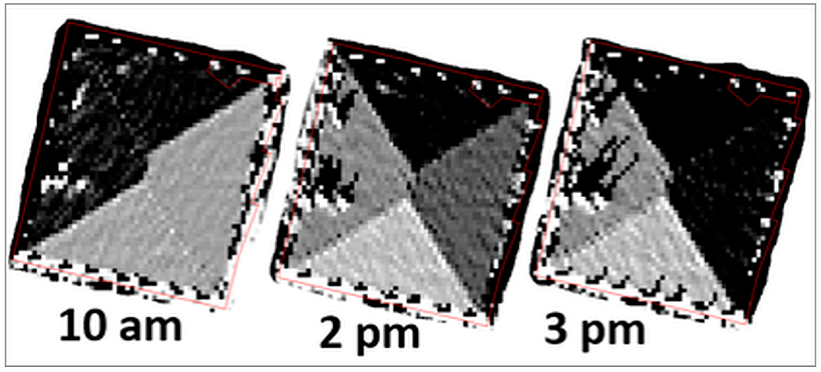
| 5 | Image detection e.g., Gaussian, Sobel, Laplace | Aerial photographs i.e., Google Earth | Only two planes of four-plane roofs distinguished. Need photos at different times of day. |
| 6 | Image supervision (supervised & unsupervised) | Aerial photographs i.e., Google Earth | Only two planes of four-plane roofs distinguished. Need photos at different times of day. |
| 7 | Hill shading with ambient occlusion | LiDAR 1 m | Generates shading patterns at different times of day. Most promising of these methods but not completely realistic. |
| Roof Characteristic | Total Systems n = 886 | |
|---|---|---|
| Percentage | Cumulative % | |
| Tilt | ||
| Model within 0–5 degrees | 61% | 61% |
| Model within 5–10 degrees | 27% | 87% |
| Model within 10–15 degrees | 9% | 97% |
| Model within 15–20 degrees | 2% | 99% |
| Azimuth | ||
| Model within 0–5 degrees | 33% | 33% |
| Model within 5–10 degrees | 19% | 52% |
| Model within 10–15 degrees | 13% | 66% |
| Model within 15–20 degrees | 9% | 74% |
| Model within 20–25 degrees | 6% | 80% |
| Model within 25–30 degrees | 6% | 86% |
| Model within 30–35 degrees | 5% | 91% |
| Model within 35–40 degrees | 4% | 95% |
| Model within 40–45 degrees | 5% | 100% |
| Size | ||
| Modelled results show minimum area | 98% | 98% |
| Model within 0–10% of actual size | 12% | 12% |
| Model within 10–20% of actual size | 9% | 21% |
| Model within 20–30% of actual size | 9% | 30% |
| Model within 30–40% of actual size | 11% | 41% |
| Model within 40–50% of actual size | 9% | 50% |
| Model within 50–60% of actual size | 9% | 59% |
| Model within 60–70% of actual size | 7% | 66% |
| Model within 70–80% of actual size | 9% | 75% |
| Model within 80–90% of actual size | 6% | 81% |
| Model within 90–100% of actual size | 6% | 87% |
| Model within 100–200% of actual size | 13% | 100% |
© 2018 by the authors. Licensee MDPI, Basel, Switzerland. This article is an open access article distributed under the terms and conditions of the Creative Commons Attribution (CC BY) license (http://creativecommons.org/licenses/by/4.0/).
Share and Cite
Palmer, D.; Koumpli, E.; Cole, I.; Gottschalg, R.; Betts, T. A GIS-Based Method for Identification of Wide Area Rooftop Suitability for Minimum Size PV Systems Using LiDAR Data and Photogrammetry. Energies 2018, 11, 3506. https://0-doi-org.brum.beds.ac.uk/10.3390/en11123506
Palmer D, Koumpli E, Cole I, Gottschalg R, Betts T. A GIS-Based Method for Identification of Wide Area Rooftop Suitability for Minimum Size PV Systems Using LiDAR Data and Photogrammetry. Energies. 2018; 11(12):3506. https://0-doi-org.brum.beds.ac.uk/10.3390/en11123506
Chicago/Turabian StylePalmer, Diane, Elena Koumpli, Ian Cole, Ralph Gottschalg, and Thomas Betts. 2018. "A GIS-Based Method for Identification of Wide Area Rooftop Suitability for Minimum Size PV Systems Using LiDAR Data and Photogrammetry" Energies 11, no. 12: 3506. https://0-doi-org.brum.beds.ac.uk/10.3390/en11123506