Using Smart Persistence and Random Forests to Predict Photovoltaic Energy Production

Abstract

Solar energy forecasting is an active research problem and a key issue to increase the competitiveness of solar power plants in the energy market. However, using meteorological, production, or irradiance data from the past is not enough to produce accurate forecasts. This article aims to integrate a prediction algorithm (Smart Persistence), irradiance, and past production data, using a state-of-the-art machine learning technique (Random Forests). Three years of data from six solar PV modules at Faro (Portugal) are analyzed. A set of features that combines past data, predictions, averages, and variances is proposed for training and validation. The experimental results show that using Smart Persistence as a Machine Learning input greatly improves the accuracy of short-term forecasts, achieving an NRMSE of 0.25 on the best panels at short horizons and 0.33 on a 6 h horizon.

1. Introduction

Solar energy forecasting is a key issue in the development of renewable energy sources. Improving the reliability and accuracy of forecasts can increase the competitiveness of solar electricity in power markets. Several methods have been proposed in recent years aiming to improve the accuracy of forecasts [1] and the solar photovoltaic grid efficiency [2,3,4,5].

Machine learning is playing an important role in the development of many new technologies, and solar forecasting techniques are no exception. Forecasting solar resources requires addressing several challenges [6]. Many advances have been made applying machine learning techniques [7,8] to solar forecasting. The main advantage of machine learning algorithms is the automatic detection of hidden patterns in large amounts of data, allowing the identification of unknown synergies and integration of varied sources of information.

This article aims to combine simple radiation predictions with real radiation measurements to predict the solar photovoltaic energy production of a diverse variety of PV modules for short-term temporal horizons. Many proposals apply machine learning algorithms to predict both photovoltaic energy production and Solar Irradiance. Orjuela-Cañón et al. [9] compare several machine learning algorithms, both linear and nonlinear, such as Regression Trees, Artificial Neural Networks, and a Seasonal Autoregressive model. Gagne et al. [10] which compares Gradient Boosting and Random forests, both of which are combinations of simple models. Diagne et al. [11] review a wide variety of statistical models, including linear and nonlinear models such as Persistence, to Artificial Neural Networks. This analysis also includes the results of models based on cloud, satellite, and ground-based images. Numerical Weather Predictors (NWPs) are also compared. Finally, Pedro and Coimbra [12] evaluate more nonlinear models exclusively using radiation data, without weather forecasts.

Common techniques used for solar forecasting are Support Vector Regression (SVR) [13], Artificial Neural Networks (ANN) [14,15,16], hybrid approaches of ANN and SVR [17,18,19] or Vector Autoregression (VAR) [20].

NWP are commonly used [21,22,23] for daily forecasts. These studies show the powerful prediction capabilities of forecasts as machine learning inputs. Furthermore, NWPs are useful when forecasting other resources, such as wind. A set of wind power predictors can be used, combining them into secondary forecasts and finally reaching the final wind forecast [24]. Wang et al. [25] use ANN to predict wind velocity using an ensemble, ANN are used. This study predicts wind velocity Using an ensemble of neural networks (Back propagation, Wavelet, Radial basis function and Generalized regression neural networks).

A common technique used in solar forecasting is Smart Persistence. This assumes the solar energy will remain constant over time. At any given point in time t, Persistence will predict into the future h minutes ahead at the time point $t+h$ as the PV energy measured in t. Therefore, Persistence follows this expression: $PV(t+h)=PV\left(t\right)$. The Persistence forecasting model is accurate on near horizons, but the accuracy decreases as the temporal horizon increases.

Smart Persistence is an improved version of Persistence which assumes the sky conditions will remain constant (instead of irradiance itself). The forecasting algorithm predicts the current solar radiation as the product of the current clear sky ratio ($K_t$) and the clear sky radiation ($I_{cs}$) in the predicted point. It is widely used as the baseline for validating more complex models and is fairly accurate in short-term horizons.

In the context of machine learning, Random Forests [26] is a classification and regression learning algorithm. A Random Forest is an ensemble learner. It trains a large number of simple decision trees and aggregates the results of every tree. Each one is trained using random subsets of the dataset to recognize different patterns and synergies in the data.

The Random Forest algorithm has been widely used in forecasting, for example Voyant et al. [7] reviews many articles in the context of machine learning applied to solar forecasting. Random Forests are rarely used for these problems, but they show very positive results whenever they are applied. The usage of this algorithm can be extended to PV production forecasting. When compared with other machine learning algorithms, Zamo [27] has argued that Random Forest (RF) is the most reliable option for forecasting PV production.

It is widely accepted that different machine learning algorithms perform differently based on the dataset used in the learning task. The RF algorithm has been chosen to forecast PV production. It has been used before in the literature and shows satisfying results on other datasets. It has been found to be the most suitable approach for the dataset tackled in this article.

This research explores the potential of introducing smart persistence predictions as inputs to machine learning forecasting techniques. The incremental methodology shown in this article demonstrates that using predictions along with past measures helps RFs find more accurate forecasts than the other methods proposed.

This article is structured as follows. First the dataset and methods used are detailed in Section 2. The features are described and then, the machine learning approach is explained. In Section 3 the experimentation is described, and the results are shown. The overall conclusions are presented in Section 4.

2. Materials and Methods

2.1. Data

The data used in this article has been provided by SunLab. The complete dataset has information on four solar stations from which Faro has been chosen. The Faro station has six different PV module models placed with optimal tilt. The data contains information on PV module temperature, meteorological variables, radiation, and PV production.

There are three years of data available with minute resolution. For short-term forecasting, minute-to-minute variations of radiation and production are very relevant. In this study, Global Horizontal Irradiance (GHI), Direct Normal Irradiance (DNI) and Photovoltaic production (PV) are used. The tested PV modules come from different manufacturers. Most of them have different PV production technology. There are six solar panel models tested labeled from A to F, panel A uses pc-Si technology, panel B uses CIS technology, panel C uses pc-Si technology, panel D uses pc-Si technology, panel E uses mc-Si technology, panel F uses CdS/CdTe thin film technology.

2.2. Method Overview

The PV production forecast problem addressed is a specific time series problem. It can be represented as the general expression for time series as presented in Equation (1).

$$PV(t+h)=f\left(PV\right(t-1),PV(t-2),\dots ,PV(t-n\left)\right)$$

(1)

In this equation, t is the time instant in minutes when the prediction is being made, h is the time horizon for which the production is being forecasted, and n is the number of time steps considered. The function f is learned and predicts PV production. In this context, the information for the t is not known, therefore any f will start with $PV(t-1)$ instead of $PV\left(t\right)$.

The general Equation (1) can be extended and further generalized to include further helpful information about weather, radiation, statistical measures, etc. This can be seen in Equation (2)

$$\begin{array}{c}\hfill PV(t+h)=f(P_1(t-1),P_1(t-2),\dots ,P_1(t-n),\\ \hfill P_2(t-1),P_2(t-2),\dots ,P_2(t-n),\\ \hfill \dots ,\\ \hfill P_m(t-1),P_m(t-2),\dots ,P_m(t-n))\end{array}$$

(2)

The data point $P_i$ is a single predictor, and m is the number of predictors that will be used. This expanded expression allows the use of more information aside from the PV production data.

Using the proposed Equation (2), a set of statistical measures and instantaneous information will be used. PV production is forecasted on horizons from 15 to 360 min and take the following values: $h=(15,30,45,60,120,180,240,300,360)$. The time steps have been set as $n=3$. These features are described in further detail in Section 2.3.

To find an adequate predictor function f the RF algorithm is used as described in Section 2.4.

2.3. Feature Description

There are two categorizations for the features considered: time window (instantaneous or aggregate) or source (measured or predicted). Instantaneous features are those taken from a single minute of the dataset. The aggregate features are a statistical transformation (mean or standard deviation) of a set of individual minute data. The source categorization consists of measured data, taken exclusively by the instruments of the power plant; or predicted data, a linear transformation of a measure that produces a rough estimation of a future value.

Given these terms, in this study ten useful predictors have been considered: Photovoltaic production (PV), GHI, DNI, mean clear sky index ($K_t$), standard deviation $K_t$, PV Smart Persistence, mean PV Smart Persistence and Standard Deviation PV Smart Persistence. All of these are classified and sorted in

Table 1. Feature classification.

	Instantaneous	Aggregate
Measured	PV production	Mean $k_t$
	GHI	Standard Deviation $k_t$
	DNI
Predicted	PV smart persistence	Mean SP
		Standard Deviation SP

.

2.3.1. PV Production

PV production is a measured and instantaneous feature, it is the energy production for a single minute of operation. It is represented as $PV\left(t\right)$. This measure is included in every model independently; it is never excluded because of the categories given.

2.3.2. GHI

GHI is a measured and instantaneous feature. It represents the amount of radiation received at a horizontal surface integrated over a single minute and its power measured as W/m${}^2$. It is represented as $I_g\left(t\right)$.

2.3.3. DNI

DNI is a measured and instantaneous feature. It represents the total amount of radiation received at a surface perpendicular to the light source integrated over a single minute and its power is measured as W/m${}^2$. It is represented as $I_d\left(t\right)$.

2.3.4. Mean $K_t$

Mean clear sky ratio ($K_t$) represents the mean $K_t$ ratio over a window of time, and it is a measured and aggregate feature. The clear sky radiation is calculated using the method proposed by European Solar Radiation Atlas (ESRA) [28]. It is commonly used as a baseline to compare more sophisticated models; however, in this research is it used to enhance the forecasting capabilities of RFs. $K_t$ is obtained by dividing $I_g\left(t\right)$ by the clear sky GHI, the theoretical maximum that $I_g\left(t\right)$ can be at any t point. This operation is shown in Equation (3), where $I_{cs}\left(t\right)$ represents the clear sky GHI.

$$K_t\left(t\right)=\frac{I_g\left(t\right)}{I_{cs}\left(t\right)}$$

(3)

The Clear Sky ratio $K_t$ removes geometrical trends that the GHI measurement due to the position of the sun in the sky. The operation that gives the feature is presented in Equation (4).

$$\overline{K_t}\left(t\right)=\frac{1}{w}{\displaystyle \sum _{i=0}^w}{K}_t(t-i)$$

(4)

where w represents the time window, in minutes. Here, it is always represented as $w=60$.

2.3.5. Standard Deviation $K_t$

Standard deviation $K_t$ is the amount of variability of the $K_t$ ratio over a window of time, and it is a measured and aggregate feature. It is calculated as presented in Equation (5)

$${\sigma }_{K_t}\left(t\right)=\sqrt{\frac{1}{w}{\displaystyle \sum _{i=0}^w}{(K_t(t-i)-\overline{K_t}(t-i))}^2}$$

(5)

2.3.6. PV Smart Persistence

PV smart persistence is the expected PV for a time point $t+h$ if the sky was as cloudy then as it is in time t. It is an instantaneous and predicted feature. This feature is an estimator of the future and it is calculated as presented in Equation (6).

$$SP(t,h)=C·K_t\left(t\right)·I_{cs}(t+h)$$

(6)

The constant C scales GHI to PV production value. It is estimated as the maximum PV power in a month, divided by the maximum GHI of the same month. This is an estimation and it is valid independently of the year it is used in. Hence, if these measures were taken for the year 2014, then it would be acceptable to reuse them again for the year 2015.

The horizon h is the minute for which the prediction is being made, and it is used in $I_{cs}(t+h)$ which is a value calculated without intervention of future knowledge.

2.3.7. Mean PV Smart Persistence

Mean PV Smart Persistence is the average value of Smart Persistence over an hour. It is an aggregate and predicted feature and it is calculated as presented in Equation (7)

$$\overline{SP}(t,h)=\frac{1}{w}{\displaystyle \sum _{i=0}^w}SP(t-i,h)$$

(7)

2.3.8. Standard Deviation PV Smart Persistence

Standard deviation PV smart persistence is the amount of variability of the PV measures over a window of time w. It is an aggregate and predicted feature and it is calculated as presented in Equation (8).

$${\sigma }_{SP}(t,h)=\sqrt{\frac{1}{w}{\displaystyle \sum _{i=0}^w}{(SP(t-i,h)-\overline{SP}(t-i,h))}^2}$$

(8)

2.4. Machine Learning

The RF algorithm is an ensemble learner. It creates a set of decision trees that vote on a final result. Since forecasting is a regression problem, instead of decision trees, a set of regression trees are trained. The forecast will be the mean of the different regression tree results. The RF algorithm is used to build the f presented in Equation (2).

Every tree of the RF is trained using independent subsets of the dataset. Each subset is built selecting data randomly from the original input dataset. The number of trees must be specified in advance, as well as how much data is taken for each subset of the initial training set. The forecast of the RF is the average of the forecasts made by the regression trees.

To get the most reliable RF, the dataset must be split in training and testing datasets. The RF algorithm is trained and tested using different partitions of the data. The training set is used in the training and parameter tuning process of the RF learning. The test set is used to extract the final metrics. There exists a training and a test set for each PV module. The training set is represented by the first three weeks of each month and the test set is represented by the leftover data after the partition is made.

This algorithm requires the adjustment of its hyper-parameters. They are the number of trees, which has been set to 500, and the randomly selected learning examples. Tuning the hyper-parameters requires a validation set. The best hyper-parameter set is selected in three steps: (1) building several models with different hyper-parameter combinations using a subset of data from the training set, (2) evaluating the models using the unused subset of data from the training set (validation set) and (3) choosing the model with the lowest error metric on the validation set. To adjust the hyper-parameters of the algorithm, a brute force search is made for each input set from Table 1 with a random seed of 1.

3. Experimentation

To test the accuracy of the different features proposed an experimentation based on the feature classification presented in Table 1 is described in this section.

The hypothesis is that adding Smart Persistence information to the time series PV forecasting will improve the accuracy metrics in a significant way. To test this, the methods and features proposed in Section 2.3 and Section 2.4 respectively, are used following the experimental methodology of Section 3.1.

3.1. Method

The whole dataset contains information for six different PV modules, thus the data is divided in six different sets that share the same irradiance measures but are different in the PV measurements. To get the final errors measurements the metrics obtained at the experimentations are the average of all PV modules accuracy metrics.

A model is trained for each PV model to analyze the performance of the ML method independently of the panel model and technology. Then the results are averaged to obtain the overall performance.

There are two main metrics used in this study, the normalized Root Mean Squared Error (RMSE) and the Skill over Smart persistence. The NRMSE is a normalized measure of the RMSE. It is relative to the average measures from the real sample. The Skill is a relative measure comparing two RMSE errors. It represents how much percentage of Smart Persistence’s RMSE needs to be added (if positive) or subtracted (if negative) to get the RMSE of the evaluated method. Higher negative numbers indicate better skill. Both are represented in Equations (9) and (10) respectively. Aside from the two main metrics proposed, two additional metrics are evaluated, the RMSE in Equation (11) and the R squared in Equation (12)

$$\mathrm{NRMSE}=\frac{\sqrt{\frac{1}{n}{\displaystyle \sum _{j=0}^n}{(p_j-d_j)}^2}}{\frac{1}{n}{\displaystyle \sum _{j=0}^n}{d}_j}$$

(9)

$$\mathrm{Skill}=\frac{\sqrt{\frac{1}{n}{\displaystyle \sum _{j=0}^n}{(p_j-d_j)}^2}}{\sqrt{\frac{1}{n}{\displaystyle \sum _{j=0}^n}{(p_j^{pers}-d_j)}^2}}-1$$

(10)

$$\mathrm{RMSE}=\sqrt{\frac{1}{n}{\displaystyle \sum _{j=0}^n}{(p_j-d_j)}^2}$$

(11)

$$\mathrm{RMSE}=1-\frac{{\displaystyle \sum _{j=0}^n}{(p_j-d_j)}^2}{{\displaystyle \sum _{j=0}^n}{(d_j-\overline{d})}^2}$$

(12)

$p_j$ and $d_j$ represent pairs of predicted and measured values. $p_j^{pers}$ represents the smart persistence prediction value. n is the number of prediction and observation pairs available.

Five different experiments are made: first dividing features by source, using only measured or predicted data, then dividing features by window, using only instantaneous or aggregate data. Finally, all features are included to build the final model. All experiments include the PV production feature.

Experiments are made with horizons up to 6 h. NWPs using Satellite and other forecasting methods are known to perform better beyond 6 h. The focus of this research is the nowcasting capabilities of integrating Smart Persistence.

3.2. Results

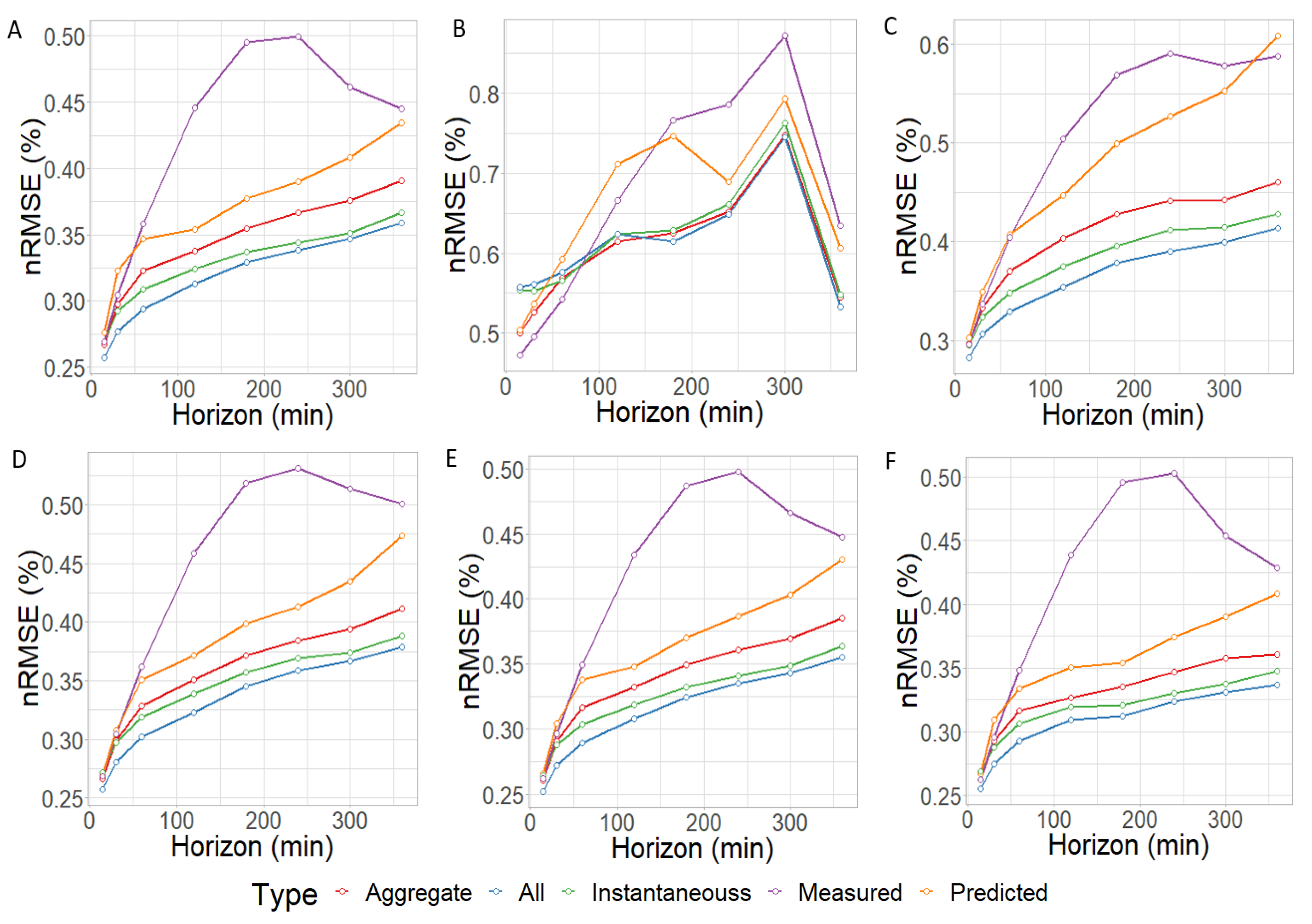
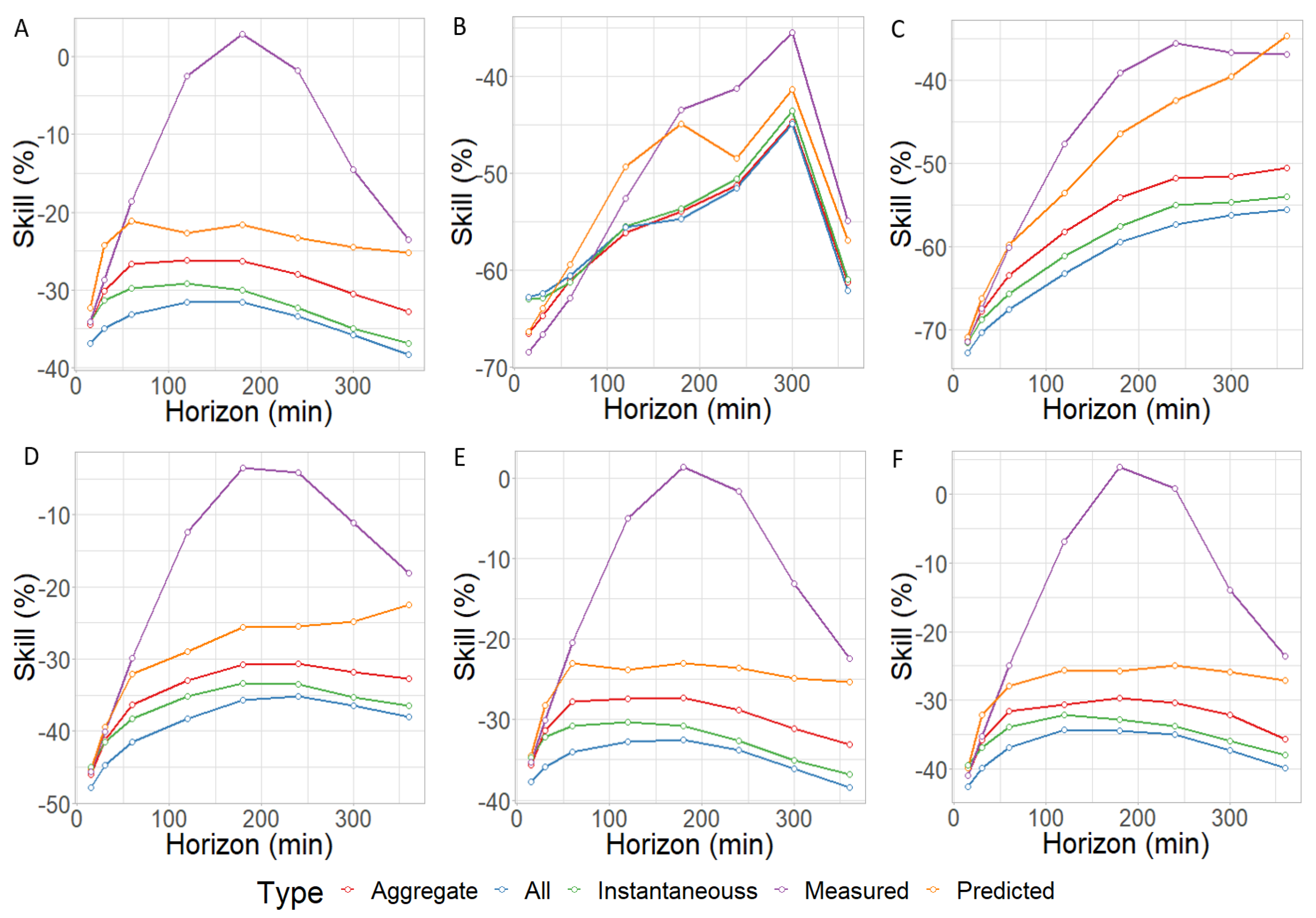
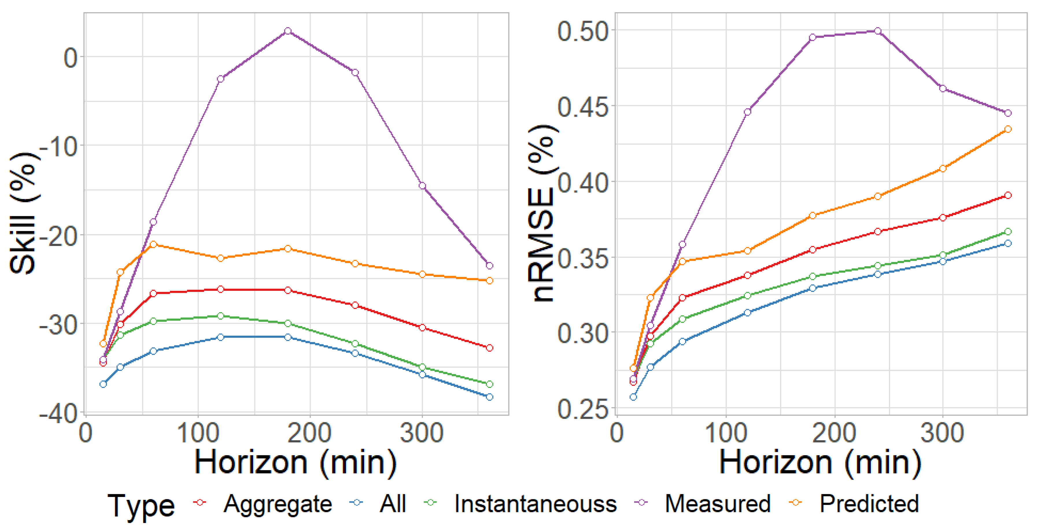
Results are shown in Figure 1, Figure 2 and Figure 3; and with

Table 2. Metric comparison of Random Forest against Linear Regression.

Model	h = 15	h = 30	h = 60	h = 120	h = 180	h = 240	h = 300	h = 360	Metric
lm	31.22	33.04	35.75	39.27	41.60	42.33	41.86	40.44	RMSE
rf	26.04	28.61	31.46	35.28	37.81	38.35	37.33	35.29	RMSE
lm	0.308	0.320	0.334	0.348	0.362	0.373	0.388	0.411	nRMSE
rf	0.257	0.277	0.293	0.312	0.328	0.338	0.346	0.358	nRMSE
lm	−24.38	−24.93	−24.09	−23.91	−24.77	−26.46	−28.01	−29.29	Skill
rf	−36.93	−34.99	−33.20	−31.64	−31.63	−33.38	−35.80	−38.29	Skill
lm	0.846	0.803	0.753	0.695	0.674	0.676	0.686	0.692	R2
rf	0.871	0.842	0.804	0.753	0.730	0.734	0.751	0.766	R2

and

Table 3. Panel metric numerical comparison.

Panel	h = 15	h = 30	h = 60	h = 120	h = 180	h = 240	h = 300	h = 360	Metric
A	26.04	28.61	31.46	35.28	37.81	38.35	37.33	35.295	RMSE
B	16.49	16.84	17.86	20.27	20.26	20.87	22.46	14.33	RMSE
C	20.74	22.94	25.64	29.38	32.22	32.86	32.01	30.29	RMSE
D	25.67	28.51	31.77	35.81	38.97	40.00	38.89	36.69	RMSE
E	26.27	28.87	31.77	35.51	38.09	38.77	37.76	35.71	RMSE
F	9.76	10.705	11.828	13.152	13.516	13.763	13.297	12.278	RMSE
A	0.257	0.277	0.294	0.313	0.329	0.339	0.347	0.359	nRMSE
B	0.558	0.56	0.577	0.624	0.615	0.648	0.745	0.533	nRMSE
C	0.283	0.307	0.329	0.354	0.378	0.39	0.399	0.414	nRMSE
D	0.258	0.281	0.302	0.323	0.345	0.359	0.367	0.379	nRMSE
E	0.252	0.272	0.289	0.308	0.324	0.335	0.343	0.355	nRMSE
F	0.255	0.274	0.293	0.309	0.313	0.324	0.331	0.337	nRMSE
A	−36.93	−34.99	−33.20	−31.64	−31.63	−33.38	−35.81	−38.29	Skill
B	−62.75	−62.37	−60.54	−55.54	−54.69	−51.56	−44.89	−62.08	Skill
C	−72.77	−70.40	−67.53	−63.24	−59.43	−57.36	−56.26	−55.54	Skill
D	−47.81	−44.79	−41.57	−38.24	−35.71	−35.19	−36.47	−38.08	Skill
E	−37.74	−35.83	−34.06	−32.71	−32.46	−33.78	−36.07	−38.39	Skill
F	−42.53	−39.84	−36.87	−34.34	−34.45	−35.01	−37.24	−39.91	Skill
A	0.872	0.842	0.804	0.754	0.73	0.735	0.751	0.766	R2
B	0.627	0.604	0.573	0.539	0.537	0.558	0.579	0.606	R2
C	0.892	0.866	0.83	0.777	0.742	0.743	0.755	0.766	R2
D	0.873	0.841	0.799	0.747	0.715	0.715	0.731	0.746	R2
E	0.87	0.84	0.803	0.755	0.731	0.734	0.75	0.764	R2
F	0.875	0.845	0.811	0.768	0.766	0.773	0.788	0.807	R2

. Figure 1 represents the NRMSE performance metric for every PV module available, Figure 2 shows the skill against performance. Here negative results correspond to the needed amount to subtract from persistence RMSE to get the RMSE of the experimented model and therefore more negative values correspond to higher forecasting accuracy. Figure 3 shows the average metrics of all PV modules. Table 2 compares two different forecasting methods, the RF approach, and a linear regression. Finally, Table 3 shows the comparison of all evaluated panel metrics, including R squared and RMSE. Both tables show results with the models constructed with every input.

It is observed that the NRMSE results are almost always lower on every PV module and horizon using the combination of all features. The exception is the PV module labeled as B, where this does not happen before the 3 h horizon. This happens both in NRMSE and Skill measurements. Excluding this exception, using all features is reliably the best option for all PV modules.

Exclusively using measurements is systematically the worst approach, being the least accurate model. It reaches very high NRMSE peaks and it is outperformed by Smart Persistence for middle horizons. The other models are frequently better than using only measured data. There is some variability on the magnitude of the metrics between PV modules. There is an ongoing trend on most panels: the best model uses every feature, followed by using instantaneous data, then aggregated data, then predicted data, and finally just measured data.

This means that using GHI, DNI and PV production just by themselves is worse than including Smart Persistence. Exclusively using predictions (both instantaneous and aggregate) is worse than using a combination of predictions and measure data. Using only aggregate or instantaneous data is worse than using a combination of both. All type of inputs presented to the RF contribute and complement each other, yielding the best results when all features are combined.

Skill metrics show similar trends to NRMSE; all PV modules behave similarly except B. However, the relative measures between PV modules vary significantly. The modules that perform best are both B and C with very high improvements. The other four PV modules evolve into worse Skill metrics, but then they start improving at the 3 h horizon. This happens because persistence is inaccurate at far horizons, but the machine learning model keeps the RMSE low enough to outperform smart persistence.

The magnitude of the Skill improvement remains very high in every model and PV module, except when using only measured data. For the best model, the improvement can go as high as 0.7 for near horizons and 0.6 for far horizons, while it never gets below 0.3 on any horizon.

The average of the metrics for each horizon shows that, even with the variance introduced by module B, using all features significantly improves results. The trends observed in individual are repeated for the averaged measurement. The main difference is that for the fifteen-minute horizon, the measured data model is just as good as the Aggregate and Instantaneous models.

Overall, the NRMSE metric appears to increase with the horizon, as is expected. It ends up doubling when using most methods. This pattern is shared by five out of the six solar panels tested. While NRMSE steadily rises through the horizons, most methods overcome Smart Persistence by a considerable margin, as shown by the Skill metric. The only time Smart Persistence is better than the ML approach is when the Measured input set is used. At the 6 h horizon, the Skill is better than at the 15 min horizon on most input sets. This is to be expected, as Smart persistence gets consistently worse as the prediction horizon increases.

A comparison between RF and linear regression (LM) is shown in Table 2. Results show that the machine learning algorithm outperforms the linear regression on all horizons and approaches. This shows that additional data by itself is not enough to get acceptable results and that machine learning significantly improves the results of forecasting. The skill metric for the linear model is high, meaning that the additional data improves predictions by a great margin independently of the model used.

Furthermore, in Table 3 all metric values are show for the best feature set. The magnitude of errors varies from panel to panel, which is very prominent on RMSE metrics. It is also shown that a high Skill metric does not convey a low error. The R squared metric for most panels (except B) is very similar when compared to the variance of the other metrics. Again, as with the Skill metric, a good R squared metric does not correlate with good prediction RMSE or nRMSE.

4. Conclusions

PV production forecasting is a relevant problem that is tackled in this article through the use of Smart Persistence as an input to a RF machine learning algorithm. Experimentation shows interesting new results. First of all, PV production forecasting depends on the PV modules analyzed. Training a RF with data from different modules will yield significantly different error metrics using the same methodology.

However, even with varied metrics, it has been shown that using only measured data is insufficient to accurately predict the future PV production for farther horizons. Estimations of future instants and trends (Smart Persistence) noticeably increases the accuracy of the machine learning models. Combining both predictions and measures has been found to be the best possible combination of features.

Further improvements could be achieved using a wider prediction window, including more accurate predictor data, or using more complex trend analysis. A wider prediction window with more instants of data might be able to improve predictions by using more relevant data. Including other powerful and more accurate predictors could guide the random forest algorithm closer to more accurate models. Finally, analyzing trends further, might allow the machine learning algorithm to estimate better predictions.

References