Electric Energy Consumption Prediction by Deep Learning with State Explainable Autoencoder

Abstract

As energy demand grows globally, the energy management system (EMS) is becoming increasingly important. Energy prediction is an essential component in the first step to create a management plan in EMS. Conventional energy prediction models focus on prediction performance, but in order to build an efficient system, it is necessary to predict energy demand according to various conditions. In this paper, we propose a method to predict energy demand in various situations using a deep learning model based on an autoencoder. This model consists of a projector that defines an appropriate state for a given situation and a predictor that forecasts energy demand from the defined state. The proposed model produces consumption predictions for 15, 30, 45, and 60 min with 60-min demand to date. In the experiments with household electric power consumption data for five years, this model not only has a better performance with a mean squared error of 0.384 than the conventional models, but also improves the capacity to explain the results of prediction by visualizing the state with t-SNE algorithm. Despite unsupervised representation learning, we confirm that the proposed model defines the state well and predicts the energy demand accordingly.

1. Introduction

As industrialization has progressed globally and the industry has developed, the demand for energy has become so high that energy has become an important topic in national policy [1]. In addition, energy use is rapidly increasing due to economic growth and human development [2]. The causes of these phenomena can be attributed to uncontrolled energy use such as overconsumption, poor infrastructure, and wastage of energy [3]. Among the demanders of various energy sources, Streimikiene estimates that residential energy consumption will account for a large proportion by 2030 [4]. According to Zuo, 39% of the United States’ total energy use is referred to as building energy consumption [5]. An energy management system (EMS) like a smart grid has been proposed to control the demand for soaring energy.

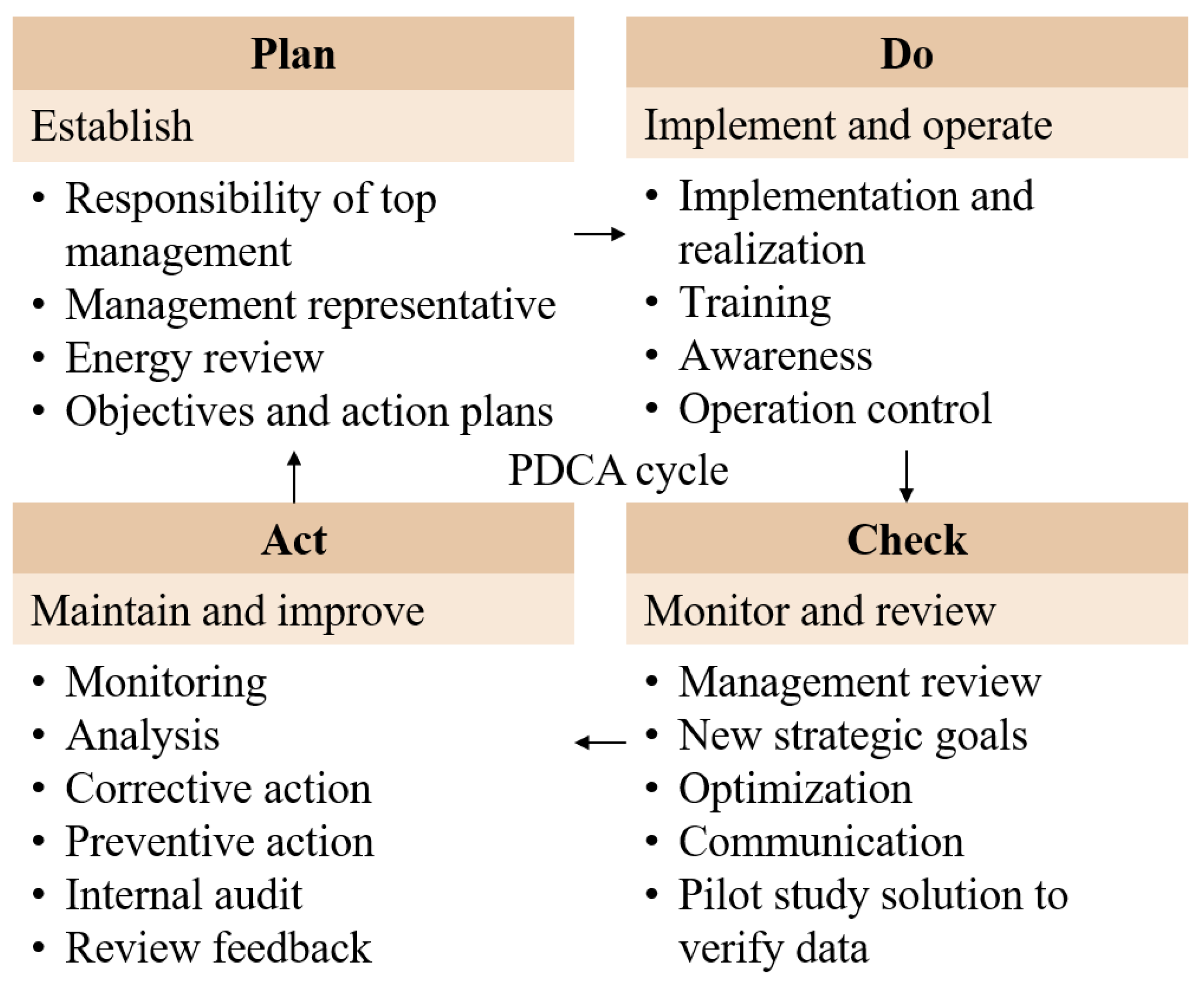
One work cycle of the EMS is the Plan-Do-Check-Act (PDCA) cycle as depicted in Figure 1 [6]. Formulating an energy plan is the first thing to do. This is the decision of the initial energy baseline, the energy performance indicators, the strategic and operative energy objectives, and the action plans. In the “do” phase, planning and action take place. The plans conducted in the previous phase have to be checked to ensure that they are effective. In the last phase, the results are reviewed, and a new strategy is established. Among the four stages, the “plan” phase is very important because it is the stage of establishing an energy use strategy and it includes an energy demand forecasting step. Therefore, it is necessary to study the energy prediction model to construct an efficient EMS.

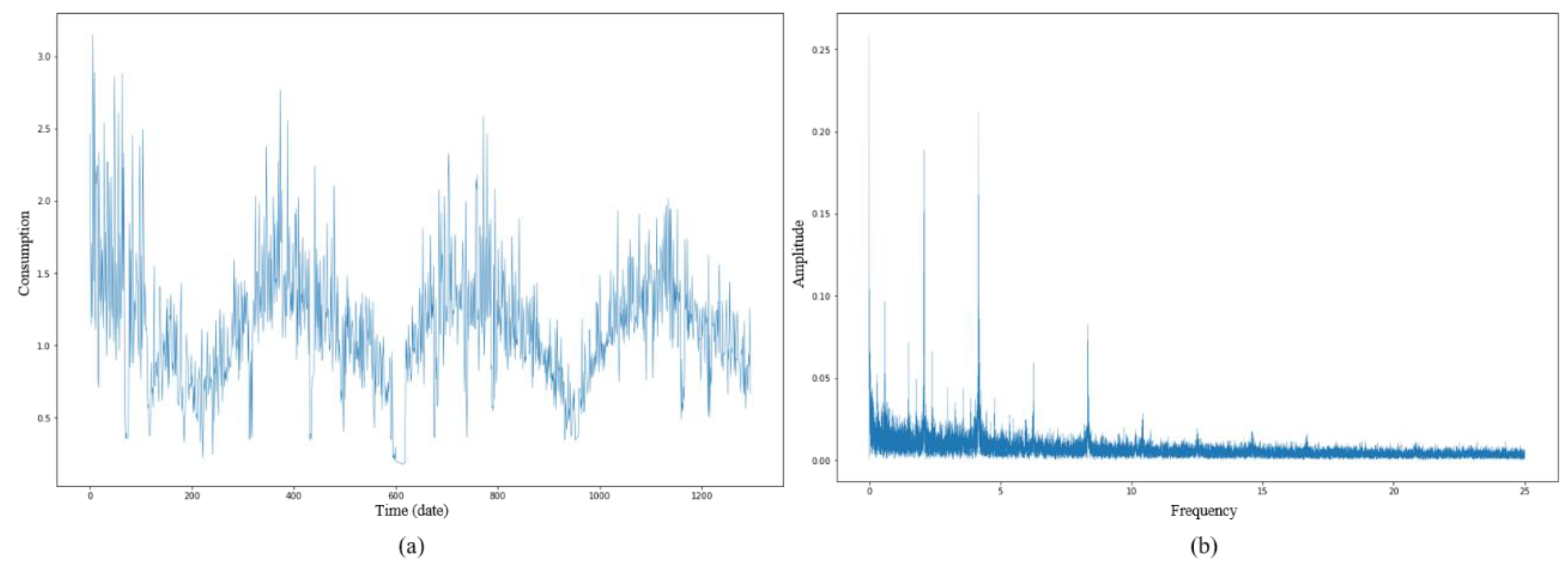
Many researchers have conducted studies with various methods to predict energy demand. In the past, machine learning techniques such as the support vector machine (SVM) and linear regression (LR) have been widely used. However, as shown in Figure 2a, energy demand values over time are complex and noisy, which limits performance. As depicted in Figure 2b, the Fourier transform to analyze patterns of energy demand reveals that it has complex features. For quantitative analysis, t-test and ANOVA were performed on the dataset used in this paper as shown in

Table 1. Results of statistical analysis of electric energy demand by month, date, and hour.

Statistical Analysis	Month	Date	Hour
p-value (t-test)	0.005	0.182	0.011
p-value (ANOVA)	0.000	6.986$\times {10}^{-56}$	0.000

. In the statistical analysis using the t-test, two groups (e.g., two different months in monthly demand) are chosen randomly and computed p-values, and we compute the average of all possible sampling. In the case of using ANOVA, p-value is computed from all the groups in each month, date, and hour.

As the result of our analysis that the characteristics of energy demand are complex, we have conducted the research with deep learning to extract difficult characteristics and work out tasks. Studies conducted using deep learning have contributed a lot to improving prediction performance, but they have not led to more utility from an energy management system perspective. If the energy demand forecasting model in the EMS copes with various situations and predicts the demand, it will be able to build a more efficient system. Therefore, in this paper, we propose a model that predicts future energy demand with that until now, considers various situations, and predicts energy demand according to different situations. This model consists of a projector that defines the state based on the energy demand to date and a predictor that predicts future energy demand from the defined state. We can adjust the automatically learned state in the middle to predict the energy demand with the consideration of various situations. The summary of the main contribution is as follows.

• We propose a novel predictive model that can be explained by not only predicting future demand for electric power but also defining current demand pattern as state.
• Our model predicts a very complex power demand value with stable and high performance compared with previous studies.
• We analyze the state defined in latent space by the proposed model and investigate a model that predicts the power demand by assuming various explanations.

The rest of the paper is as follows. Section 2 introduces the previous studies for forecasting energy demand and addresses the limitations. To overcome these shortcomings, we propose our model in Section 3. Section 4 shows the results of the energy demand forecasting with the proposed model and also shows the result of forecasting the demand by considering various situations. In the final section, conclusions and discussion are presented.

2. Related Works

Several studies have been conducted to predict energy demand mentioned in Section 1.

Table 2. The summary of related works.

Category	Author	Method	Description
Statistical model	Munz et al. (2007)	K-means clustering	Calculate the center value of the cluster and classify the time series into regular and irregular trend
	Kandananond (2011)	ARIMA	Present different forecasting methods to predict electricity consumption
	Cauwer et al. (2015)	Statistical model and its physical principles	Apply statistical method of multiple linear regression to real-world trip and energy consumption data
Machine learning model	Dong et al. (2005)	Support vector machine	Predict building energy demand in the tropical region using SVM
	Gonzalez and Zamarreno (2005)	Feedback neural network	Present a simple model to predict electric load in buildings
	Ekici and Aksoy (2009)	Artificial neural network	Forecast buildings energy needs benefitting from orientation, insulation thickness and transparency ratio using ANN
	Li et al. (2010)	Support vector machine	Forecast annual energy demand using the building’s heat transfer coefficient
	Xuemei et al. (2010)	Fuzzy support vector machine, Fuzzy c-means clustering	Present a novel short-term cooling load forecasting with conjunctive use of fuzzy C-mean clustering to define state and fuzzy SVM for prediction
	Ma (2010)	Linear regression	Propose model based on linear regression that predicts large-scale public building energy demand
Deep learning model	Ahmad et al. (2017)	Deep neural network	Forecast energy demand with information of climate, date, and building usage rate
	Lee et al. (2017)	Recurrent neural network	Measure the environmental consumption level for each country with a pro-environmental consumption index using big data queries
	Li et al. (2017)	Autoencoder	Extract the building energy demand and predict future energy consumption

summarizes the previous studies. In the past, statistical techniques were used mainly to predict energy demand. Munz et al. predicted a time series of irregular patterns using k-means clustering [7]. Kandananond used different forecasting methods—autoregressive integrated moving average (ARIMA), artificial neural network (ANN), and multiple linear regression (MLR) —to predict energy consumption [8]. Cauwer et al. proposed a method to predict energy consumption using a statistical model and its underlying physical principles [9].

However, due to the irregular patterns of energy demand, statistical techniques have limited performance and many models of prediction using machine learning methods have been investigated. Dong et al. predicted the demand of building energy using SVM with consumption and weather information [10]. Gonzalez and Zamarreno forecasted the next temperature from the temperature to date using a feedforward neural network (NN) and predicted the requirement with the difference of them [11]. Ekici and Aksoy predicted the building energy needs with properties of buildings without weather conditions [12]. Li et al. estimated the annual energy demand using SVM with the building’s transfer coefficient [13]. However, these studies only constructed models to predict correct value corresponding to the input so as to lack the basis for influence of the input features. To solve this problem, Xuemei et al. set the state for forecasting energy consumption through fuzzy c-means clustering and predicted demand with fuzzy SVM [14]. Ma forecasted energy consumption with specific population activities or unexpected events, as well as weather condition as inputs of the MLR model [15]. Although the above studies set the state and forecasted future consumption based on it, they lacked the mechanism to identify the state accurately.

As mentioned in Section 1, the energy consumption data contain large noise. Deep learning, which is a rising method to solve complex tasks of late, is efficient for predicting energy demand because it solves tasks by modeling complex characteristics of data well [16]. Ahmad et al. forecasted energy demand by constructing a deep NN and inputting the information of weather and building usage rate [17]. Lee et al. estimated environmental consumption by using a temporal model like recurrent neural network (RNN) with energy consumption data and temporal features [18]. Li et al. proposed a method to predict energy demand with autoencoder, one of the methods to represent data [19]. However, Li et al.’s model included only fully-connected layers, so that temporal features were ignored, and it is hard to control the conditions because latent space where the features of data are represented is not defined in that model.

Although some of the above studies provided novel research directions, other features such as information of weather and building are used in addition to the energy demand value, which is costly to construct the model for energy consumption prediction. Besides, they lack the explanation capability on the predicted value, because there was no study on the state to analyze the results of prediction. However, studies that analyze and explain the predictive results are essential for practical use of the predictive model. In this paper, we propose a model that visualizes a state by defining the state based on the current usage pattern and date information, so as to be able to explain the results of prediction. Our model, like any other prediction models, takes the energy demand up to now as input and predicts consumption in the future. However, in order to overcome the limitations of the end-to-end system, which cannot analyze the internal prediction process, we add a step to define the state of the demand pattern in the middle.

3. Proposed Method

3.1. Overview

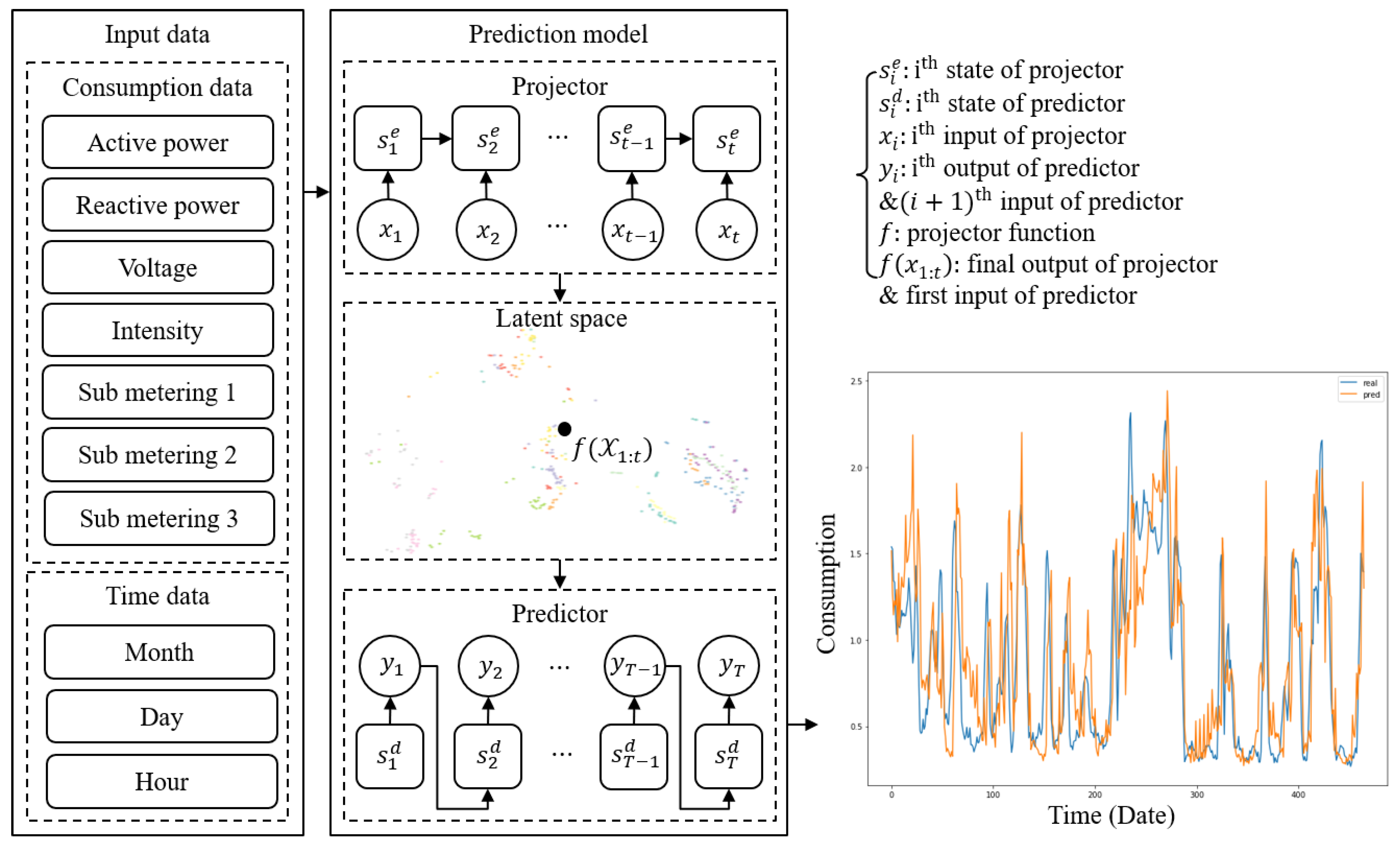
As mentioned in Section 1 and Section 2, nonlinear approaches, including those based on fuzzy and neural net, have demonstrated successful performance in many applications [20,21,22,23]. In this paper, we have contributed to the field of application by solving the power demand forecasting problem using the deep neural network-based method. Compared to the previous work, the overall architecture of our model consists of a projector $f$ and a predicter $g$, similar to an auto-encoder consisting of an encoder and a decoder as shown in Figure 3 [24]. There are many ways to deal with time series data, but $f$ and $g$ are based on long short-term memory (LSTM), one of the RNN’s, to handle time series data [25,26,27,28]. Predictor uses the output value of each time-step as the input of the next [29]. The projector defines the state by compressing the energy demand and transferring it to the latent space representing the demand information. Predictor predicts future energy demand based on the defined state. It can be done by end-to-end learning of the projector and the predictor, and the process of defining state is trained automatically. In the variational autoencoder (VAE), the state defined on the latent space contains the feature of the produced data, and also contains the information of the expected energy consumption, as well as features of the input values [30,31]. Ma and Lee predicted the energy consumption by adding more information of the surrounding environment while learning [15,18]. However, unlike them, after learning to predict the consumption with only demand to date, our model can predict future consumption by adjusting the state on the latent space with the condition of the surrounding environment.

3.2. Consumption Representation

Previous studies have constructed a model that sends energy consumption $\mathcal{X}$ to a predicted value $\mathcal{Y}$ as in Equation (1), while we define a state by adding a potential space $\mathcal{S}$ between $\mathcal{X}$ and $\mathcal{Y}$, as shown in Equation (2).

$$f:\mathcal{X}\to \mathcal{Y}$$

(1)

$$f:\left(\mathcal{S},\mathcal{X}\right)\to \mathcal{S}$$

(2)

We continuously update the state during the time interval t. The state $s_i^e$ for $i$ during the time interval t of input is defined as follows.

$$s_i^e=f\left(x_i^e,s_{i-1}^e\right),$$

(3)

where e means “embedded state”, $x_i^e$ is the ith input value of projector and $s_0^e=0$. $f\left(\cdot ,\cdot \right)$ is a LSTM for the projector including one memory cell $c_t$ and three gates (input $i_t$, forget $f_t$, and output $o_t$). We calculate each value as follows.

$$s_t^e=o_t\ast tanh{c}_t,$$

(4)

$$o_t=\sigma \left(U_o\ast x_t^e+W_o\ast s_{t-1}^e\right),$$

(5)

$$c_t=f_t\ast c_{t-1}+I_t\ast {\overline{c}}_t,$$

(6)

$$I_t=\sigma \left(U_I\ast x_t^e+W_I\ast s_{t-1}^e\right),$$

(7)

$$f_t=\sigma \left(U_f\ast x_t^e+W_f\ast s_{t-1}^e\right),$$

(8)

$${\overline{c}}_t=tanh\left(U_c\ast x_t^e+W_c\ast s_{t-1}^e\right),$$

(9)

where $U$ and $W$ are weights of the layer, $\sigma$ is activation function, and $\overline{c}$ and $\mathrm{c}$ are intermediary memory cell and memory cell, respectively. We set $s_t^e$ as the last state of the projector (i.e., $s_t^e=f\left(x_t^e,s_{t-1}^e\right)$). The process to define the state is learned automatically as the predictor interacts with the projector to predict the demand. The details are introduced in the next section.

The state of the projector is located on the latent space where patterns and features of input energy consumption are shown. Therefore, by controlling the state transferred to the latent space, it is possible to predict the future consumption as well as to analyze the current consumption situation.

3.3. Demand Prediction

This section presents how to use the state set by the projector for forecasting future demand. First, as shown in Equations (10) and (11), the predictor predicts a single consumption value immediately after inputting the state. Recursively, predictor forecasts the next single demand value with the predicted value.

$$g:\left(\mathcal{Y},\mathcal{S}\right)\to \mathcal{Y},$$

(10)

$$s_i^d=g\left(y_{i-1},s_{i-1}^d\right),$$

(11)

where d means “demand”, $y_i$ is the ith output and the (i + 1)th input of predictor at the same time, and $y_0=0$. $g\left(\cdot ,\cdot \right)$ is a RNN for the predictor. It gets the output of itself from the previous time-step as input and is computed as follows.

$$s_i^d=\sigma \left(U_s\ast y_{i-1}+W_s\ast s_{i-1}^d+b_s\right)$$

(12)

$$y_i=U_y\ast s_i^d+b_y$$

(13)

Since the predictor forecasts the demand based on the first input state, if the state is arbitrarily controlled by the user, the model can predict the demand according to various conditions, resulting in an effective energy management system. For example, adding different conditions, such as information of weather or economy, can make energy demand prediction model more smoothly.

To train the proposed model, we use L2 loss function as shown in Equation (14) by sampling the data with a time interval of $t$ and $T$ in $\mathcal{X}$ and $\mathcal{Y}$, respectively. The projector interacts with the predictor and learns to automatically define the state.

$$\mathsf{ℒ}={\mathbb{E}}_{\left(x_{1:t},y_{1:T}\right)\sim \left(\mathcal{X},\mathcal{Y}\right)}\left[{\left(y_{1:T}-g(f(x_{1:t}))\right)}^2\right]$$

(14)

The algorithms for learning the proposed model and forecasting the future demand are as follows. In Algorithm 1, two functions $f$ and $g$ are trained with energy demand record for t minutes,$x_{1:t}$, and energy demand to be predicted for $T$ minutes, $y_{1:T}$. In Algorithm 2, at first, we get a state with energy consumption ${\mathrm{x}}_{1:\mathrm{t}}$ and the predictor $f$. Then, based on the computed state $s_t^e$, we predict total T minutes by 1 min with the predictor $g$.

Algorithm 1. Learning algorithm for the proposed method

Input: Dataset ($\mathcal{X},\mathcal{Y})$ Output: Trained model $f,g$ Initialize projector $f$ and predictor $g$; repeat  Sample ${\mathrm{x}}_{1:\mathrm{t}},{\mathrm{y}}_{1:\mathrm{T}}$ from $\mathcal{X},\mathcal{Y}$, respectively;  ${\theta }_f\leftarrow {\theta }_f-\frac{\partial }{\partial {\theta }_f}\left(\mathsf{ℒ}\right)$;  ${\theta }_g\leftarrow {\theta }_g-\frac{\partial }{\partial {\theta }_g}\left(\mathsf{ℒ}\right)$; until${\theta }_f,{\theta }_g$ converge return$f,g$

where ${\theta }_f,{\theta }_g$ are parameters of projector $f$ and predictor $g$, respectively.

Algorithm 2. An algorithm to predict electric energy demand

Input: $x_{1:t}$ Output: $y_{1:T}$ for$i=1,\dots t$ do  $s_i^e\leftarrow f\left(x_i,s_{i-1}^e\right)$; end for  ${\mathrm{s}}_1^d\leftarrow f_d\left(y_0,s_t^e\right)$;  $y_1\leftarrow U_y\ast s_1^d+b_y$; for$i=2,\dots ,T$do  $s_i^d\leftarrow g\left(y_{i-1},s_{i-1}^d\right)$;  $y_i\leftarrow U_y\ast s_i^d+b_y$; end for return$y_{1:T}$

3.4. State Transition

This section describes how the user can arbitrarily adjust the defined state to assume various situations and predict energy demand. When energy demand $x_A$ based on condition A (e.g., warm weather) comes in as input, and when predicting energy demand based on condition B (e.g., cold weather), first, the average of state $\overline{s_A}$ of the demanded quantities of condition A and the average $\overline{s_B}$ of states of the demanded quantities of condition B are calculated. If the state $s_A$, which is defined by inputting $x_A$ to projector, is subtracted from $\overline{s_A}$ and $\overline{s_B}$ is added to the state calculated through the energy demand $x_A$, it can be seen that the condition A is omitted, and the condition B is added. We perform the state transition with this process and forecast the energy demand according to various conditions.

4. Experiments

4.1. Dataset amd Experimental Settings

To verify the proposed model, we use a dataset on household electric power consumption [32]. There are about two million minutes of electric energy demand data from 2006 to 2010, and they are divided into training and test data as a 9:1 ratio. It consists of eight attributes including date, global active power (GAP), global reactive power (GRP), global intensity (GI), voltage, sub metering 1, 2, and 3 (S1, 2, and 3), and the model predicts the GAP. S1 corresponds to the kitchen, containing mainly a microwave, an oven, and a dishwasher. S2 corresponds to the laundry room, containing a refrigerator, a tumble-drier, a light, and a washing-machine. S3 corresponds to an air-conditioner and an electric water-heater. The statistical summary of each feature is described in

Table 3. The summary of the data used in this paper.

Attribute	Date	GAP (kW)	GRP (kW)	Voltage (V)	GI (A)	S1	S2	S3
Average	-	1.089	0.124	240.844	4.618	1.117	1.289	6.453
Std. Dev	-	1.055	0.113	3.239	4.435	6.139	5.794	8.436
Max	26/11/2010	11.122	1.390	254.150	48.400	88.000	80.000	31.000
Min	16/12/2006	0.076	0.000	223.200	0.200	0.000	0.000	0.000

.

To train the time series model, we use a backpropagation through time (BPTT) algorithm, and the Adam optimizer with default hyper parameters in the keras library of python [33,34]. All weights are initialized with Glorot initialization [35]. The operating system of the computer used in our experiments was Ubuntu 16.04.2 LTS and the central processing unit of the computer was an Intel Xeon E5-2630V3. The random-access memory of the computer was Samsung DDR4 16 GB × 4, and the graphic processing unit of the computer was GTX Titan X D5 12 GB. The number of hidden units in the deep learning approach, including our model (i.e., the size of the state $s$) was set at 64.

4.2. Demand Prediction

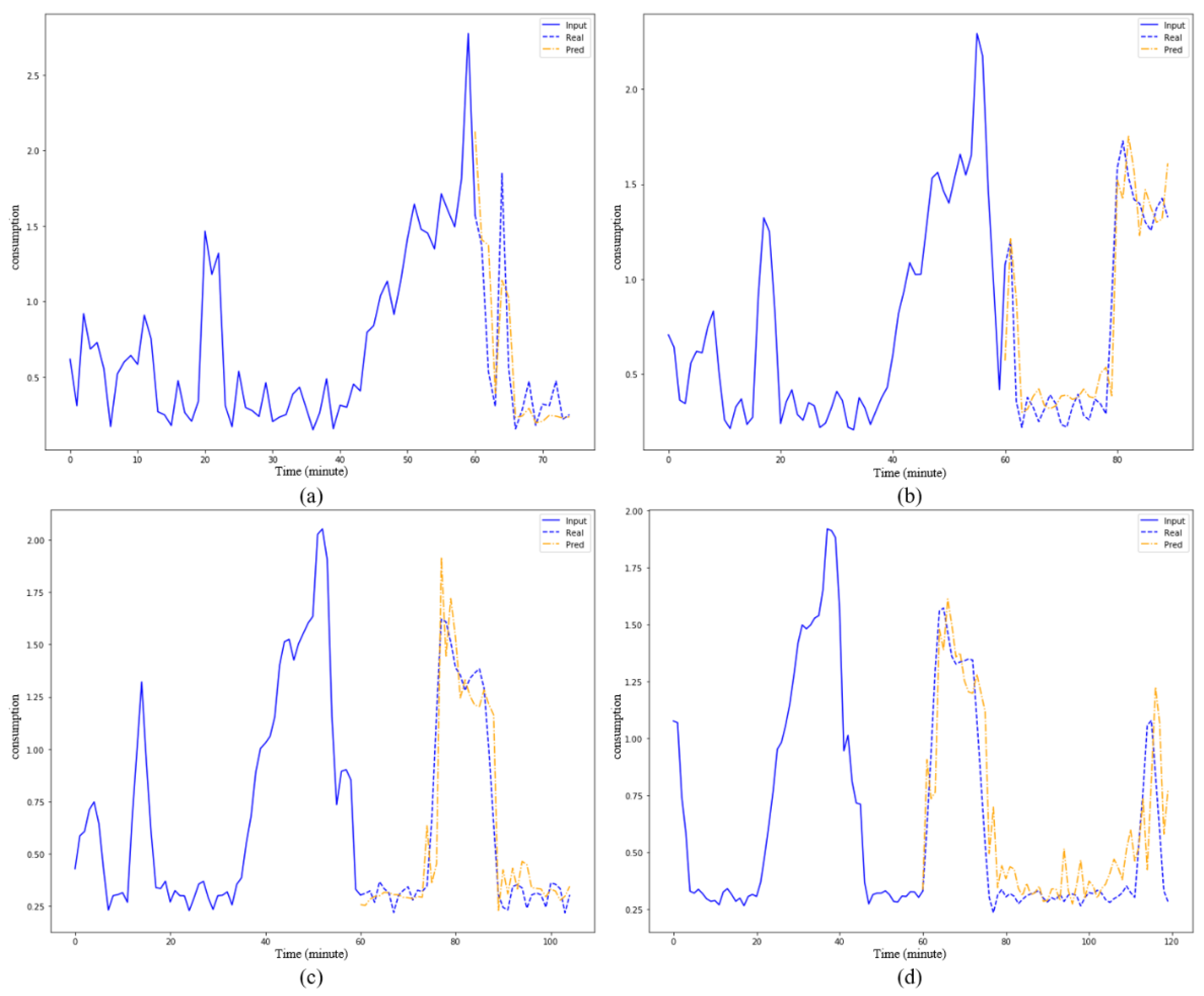
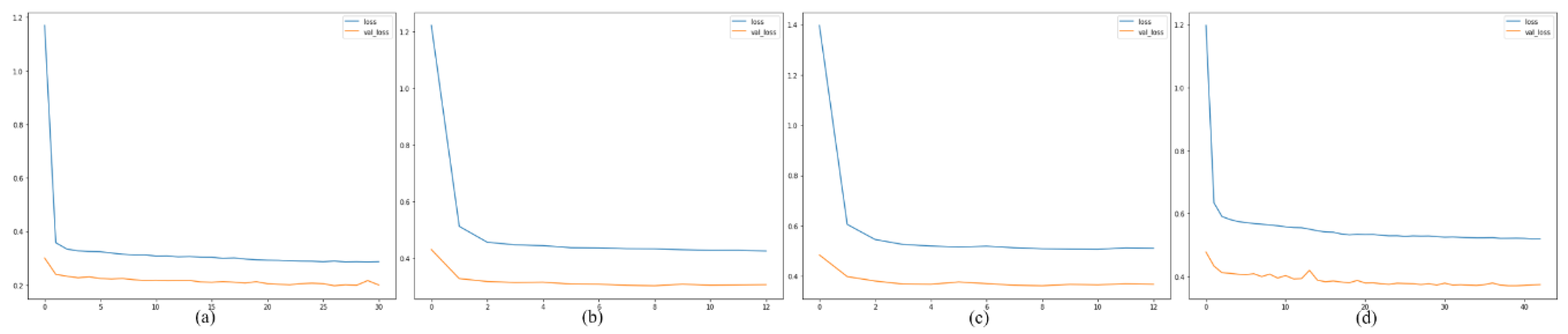
To verify the performance of the proposed model, we show the energy demand forecasting result using our model and compared with other conventional methods. Figure 4 is the result showing real and predicted energy demand values at the same time. The model predicts energy demand for 15, 30, 45, and 60 min with actual energy demand for 60 min. Although the model could not predict the energy demand perfectly, we confirm that the energy demand pattern predicted well. We show the convergence of the learning algorithm experimentally by showing the change of loss value as learning progresses in Figure 5.

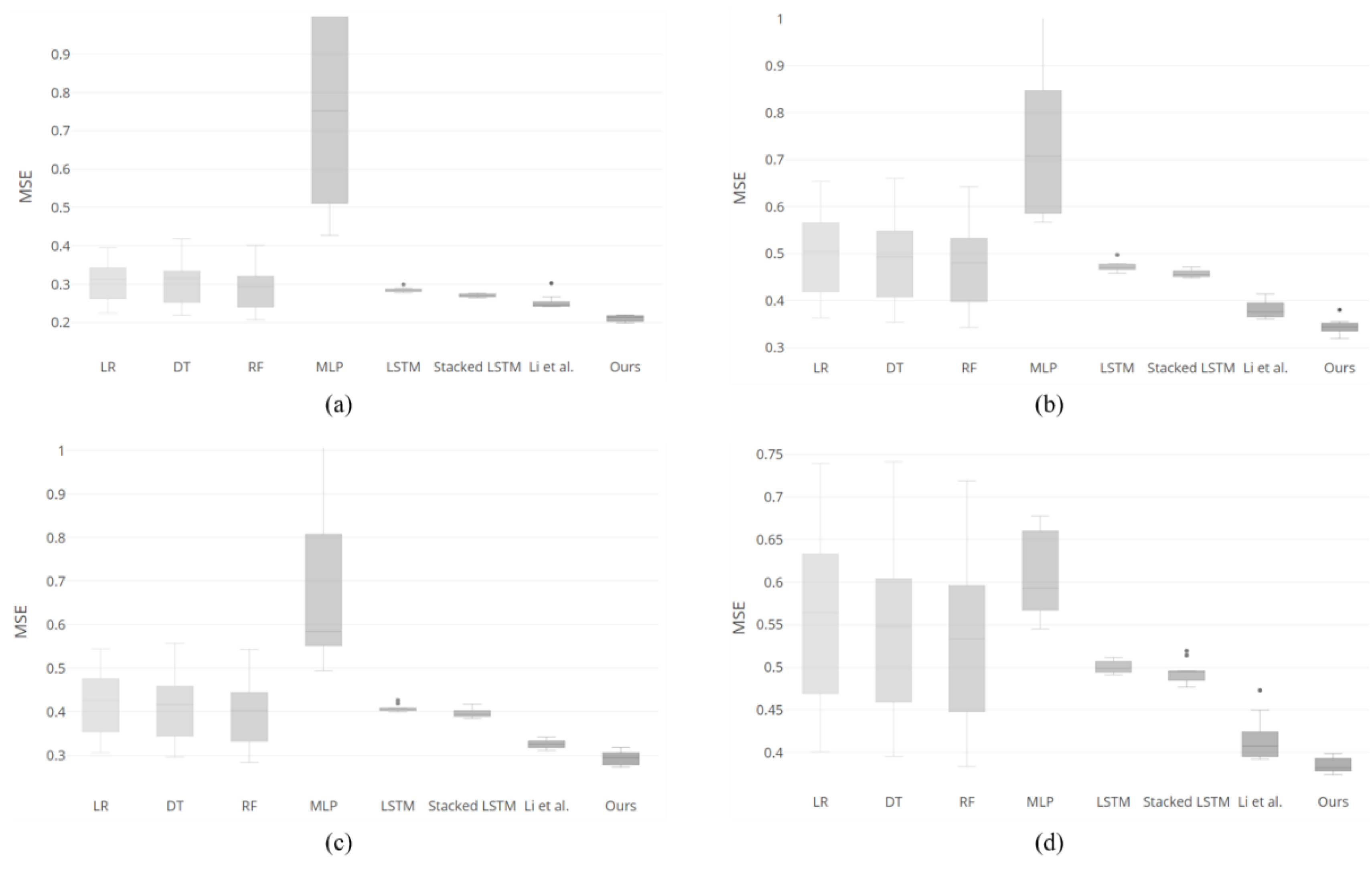
Our model is compared with conventional machine learning methods such as linear regression (LR), decision tree (DT), random forest (RF) and multilayer perceptron (MLP), and with deep learning methods such as LSTM, stacked LSTM, and the autoencoder model proposed by Li. Stacked LSTM is a model including two LSTM layers similar to our model but does not set the state. A model proposed by Li has one hundred hidden units and four hidden layers. The MSE measure of the experimental results for each model is shown in Figure 6 as box plot. The results of the comparison with other models show that the proposed model outperforms other models. We can confirm that the conventional machine learning methods (LR, DT, RF, and MLP) show a large variation in prediction performance, but the deep learning methods (LSTM, Stacked LSTM, the Li’s model, and ours) are trained in stable. Some of the deep learning methods are worse than machine learning methods, but our model yields the best performance.

To examine the performance of the prediction model, we use three evaluation metrics—the mean squared error (MSE), the mean absolute error (MAE), and the mean relative error (MRE), which can be calculated respectively as follows.

$$MSE=\frac{1}{N}{\Sigma }_{i=1}^N{\left({\widehat{y}}_m-y_m\right)}^2$$

(15)

$$MAE=\frac{1}{N}{\Sigma }_{i=1}^N\left|{\widehat{y}}_m-y_m\right|$$

(16)

$$MRE=\frac{1}{N}{\Sigma }_{i=1}^N\frac{\left|{\widehat{y}}_m-y_m\right|}{y_m}$$

(17)

We conducted the experiments with 10-fold cross validation and the average values for each metric are shown in

Table 4. The numerical results of experiments. Our model outperforms the other models in most metrics.

Metric	LR	DT	RF	MLP	LSTM	SLSTM	Li et al.	Ours
15 min
MSE	0.3077	0.3092	0.2915	2.0992	0.2853	0.2704	0.2531	0.2113
MAE	0.2878	0.2841	0.2758	1.0580	0.3206	0.3119	0.3191	0.2517
MRE	0.3925	0.3910	0.3719	2.2327	0.5021	0.4886	0.5706	0.3625
30 min
MSE	0.4201	0.4125	0.3992	0.7315	0.4084	0.3964	0.3256	0.2937
MAE	0.3657	0.3585	0.3511	0.6318	0.4232	0.4101	0.3581	0.3315
MRE	0.5343	0.5165	0.5079	1.2325	0.7131	0.6778	0.6004	0.5399
45 min
MSE	0.4982	0.4879	0.4757	0.7462	0.4720	0.4581	0.3808	0.3450
MAE	0.4210	0.4097	0.4033	0.6442	0.4742	0.4559	0.4120	0.3700
MRE	0.6462	0.6077	0.6012	1.2613	0.8274	0.7668	0.7441	0.6612
60 min
MSE	0.5573	0.5457	0.5322	0.7621	0.4997	0.4945	0.4159	0.3840
MAE	0.4626	0.4470	0.4409	0.6260	0.4946	0.4924	0.4404	0.3953
MRE	0.7356	0.6828	0.6762	1.2161	0.8871	0.8916	0.8129	0.6478

.

4.3. State Transition

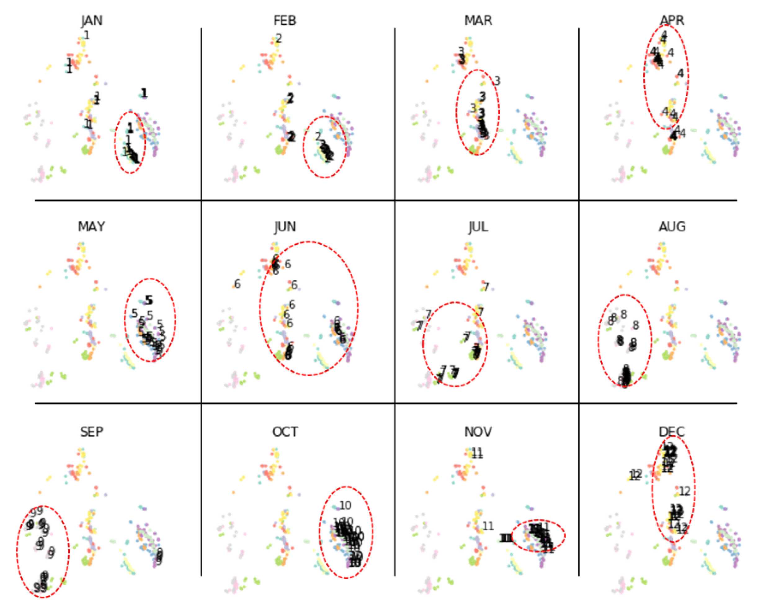
We empirically verify whether our model can automatically learn a capacity to define state as described in Section 3. We extract the output of the projector to get states and visualize them as shown in Figure 7. We use the t-SNE algorithm to visualize the state [36]. We confirm that the consumption data are not separated clearly by month, but they are clustered by month on the latent space even with the unsupervised representation learning. Approximately the distribution of data can be divided into right (January, February, May, October, and November), left (August and September), top (December), center (March), center-right (June), center-left (July), and center-top (April). We mark plotted points of each month with annotations to figure and illustrate it monthly to show the state for each month, resulting in twelve plots. It can be seen that the defined state is well clustered on a monthly basis, achieving low intra-class variability.

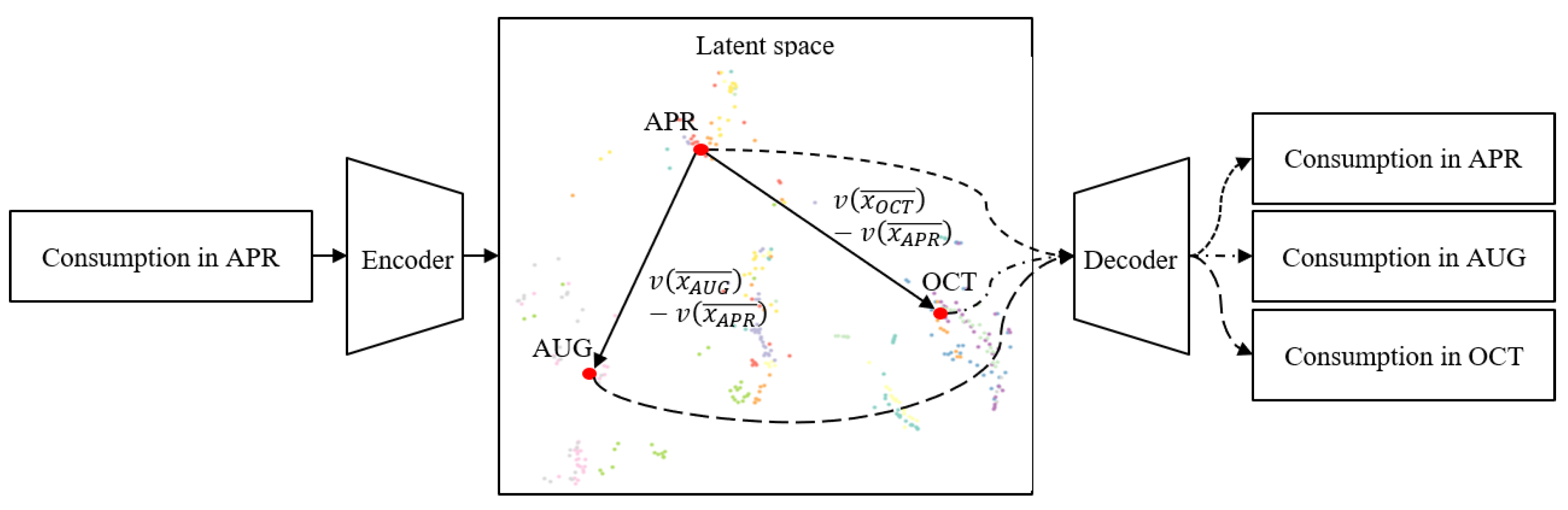
Our model is also empirically confirmed that not only defines the state well but also has the capacity to adjust the prediction by controlling the state on latent space. This method is effective for EMS, for example, because the electricity demand prediction can be made flexible according to the climate or economic situation. The experiment to control the condition of the month is conducted, and other conditions are left for future study. An example of a state transition that controls a state on the latent space is shown in Figure 8. If we want to forecast the energy demand in October with only consumption in April, we just project the demand in April into the latent space to extract the state. After extracting the state for the electric energy consumption at one point in April, we add the average value of the states for October $v\left(\overline{x_{OCT}}\right)$ and subtract the average value of the states for the April $v\left(\overline{x_{APR}}\right)$ and put it into the predictor to get the predicted values.

Table 5. The results of experiments on state transition. Each column shows the month of the input electric energy demand and each row shows an output month after state transition. The ground truth (G.T.) is the average electric energy consumption for each month.

	JAN	FEB	MAR	APR	MAY	JUN	JUL	AUG	SEP	OCT	NOV	DEC	G.T.
JAN	-	1.333	1.365	1.391	1.374	1.339	1.313	1.314	1.329	1.341	1.345	1.379	1.389
FEB	1.195	-	1.157	1.173	1.158	1.126	1.083	1.075	1.084	1.093	1.115	1.183	1.116
MAR	1.163	1.070	-	1.141	1.123	1.093	1.038	1.049	1.050	1.052	1.076	1.147	1.131
APR	1.189	1.104	1.158	-	1.151	1.122	1.071	1.068	1.074	1.084	1.108	1.174	1.176
MAY	1.199	1.123	1.160	1.184	-	1.134	1.090	1.067	1.075	1.094	1.120	1.189	1.159
JUN	1.300	1.242	1.269	1.287	1.272	-	1.229	1.208	1.222	1.234	1.243	1.289	1.244
JUL	0.903	0.818	0.823	0.817	0.828	0.806	-	0.763	0.764	0.770	0.798	0.893	0.786
AUG	0.694	0.601	0.584	0.561	0.585	0.576	0.537	-	0.517	0.548	0.575	0.687	0.511
SEP	0.796	0.699	0.695	0.677	0.697	0.684	0.637	0.620	-	0.647	0.679	0.791	0.623
OCT	0.917	0.829	0.836	0.828	0.835	0.818	0.766	0.750	0.754	-	0.818	0.920	0.779
NOV	1.020	0.928	0.953	0.956	0.950	0.929	0.866	0.852	0.854	0.876	-	1.022	0.923
DEC	1.275	1.202	1.248	1.283	1.248	1.221	1.175	1.150	1.162	1.187	1.208	-	1.265

shows the average value of the predicted electric power consumption for one hour in minutes to determine whether the demand pattern for April is changed to the consumption pattern for October after the state transition. Each column shows the month of the input electric energy demand to date, and each row shows an output month of state transition to predict the desired pattern for the specified month. The ground truth (GT) is the average electric energy consumption for each month. It can adjust the state on the latent space because the predicted consumption after conditioning is similar to GT.

5. Conclusions

We have addressed the importance of energy demand prediction and proposed a model to solve them. It attempts to predict electric energy consumption through defining the state unlike the conventional machine learning or deep learning models. Divided into two parts (projector and predictor), each part interacts with the other and learns to automatically set a state without any supervision. We achieve the best forecasting performance compared to others, analyze the state, and peek the basis for the predicted consumption value. In addition, the state transition method shows that our model can be more efficient because we can control the predicted electric energy consumption values according to various situations by adjusting conditions. For example, if we add several conditions to the state such as information of weather or economy, we can predict electricity demand accordingly.

In this paper, we have conducted experiments with several conditions of the state only for the month. We will experiment with various conditions such as weather, economy, or any other events in the future works. In this paper, only the energy consumption of one individual household is predicted, so the demand of several buildings will be collected, and we will add the information about building into the state and have a plan to propose a model which can predict energy consumption of various buildings. Finally, we will construct an efficient energy management system including the proposed prediction model.

References

- Oluklulu, Ç. A Research on the Photovoltaic Modules That Are Being Used Actively in Utilizing Solar Energy, Sizing of the Modules and Architectural Using Means of the Modules. Master’s Thesis, Gazi University, Ankara, Turkey, 2001. [Google Scholar]
- Ugursal, V.I. Energy Consumption, Associated Questions and some Answers. Appl. Energy 2014, 130, 783–792. [Google Scholar] [CrossRef]
- Rinkesh. What is the Energy Crisis. Available online: https://www.conserve-energy-future.com/causes-and-solutions-to-the-global-energy-crisis.php#abh_posts (accessed on 25 January 2019).
- Streimikiene, D. Residential Energy Consumption Trends, Main Drivers and Policies in Lithuania. Renew. Sustain. Energy Rev. 2014, 35, 285–293. [Google Scholar] [CrossRef]
- Zuo, J.; Zhao, Z.Y. Green Building Research-Current Status and Future Agenda: A review. Renew. Sustain. Energy Rev. 2014, 30, 271–281. [Google Scholar] [CrossRef]
- Prashar, A. Adopting PDCA (Plan-Do-Check-Act) Cycle for Energy Optimization in Energy-Intensive SMEs. J. Clean. Prod. 2017, 145, 277–293. [Google Scholar] [CrossRef]
- Munz, G.; Li, S.; Carle, G. Traffic Anomaly Detection Using k-means Clustering. In Proceedings of the GI/ITG Workshop MMBnet, Hamburg, Germany, 13–14 September 2007; pp. 13–14. [Google Scholar]
- Kandananond, K. Forecasting Electricity Demand in Thailand with an Artificial Neural Network Approach. Energies 2011, 4, 1246–1257. [Google Scholar] [CrossRef]
- De Cauwer, C.; Van Mierlo, J.; Coosemans, T. Energy Consumption Prediction for Electric Vehicles based on Real-world Data. Energies 2015, 8, 8573–8593. [Google Scholar] [CrossRef]
- Dong, B.; Cao, C.; Lee, S.E. Applying Support Vector Machines to Predict Building Energy Consumption in Tropical Region. Energy Build. 2005, 37, 545–553. [Google Scholar] [CrossRef]
- Gonzalez, P.A.; Zamarreno, J.M. Prediction of Hourly Energy Consumption in Buildings Based on a Feedback Artificial Neural Network. Energy Build. 2005, 37, 595–601. [Google Scholar] [CrossRef]
- Ekici, B.B.; Aksoy, U.T. Prediction of Building Energy Consumption by Using Artificial Neural Networks. Adv. Eng. Softw. 2009, 40, 356–362. [Google Scholar] [CrossRef]
- Li, Q.; Ren, P.; Meng, Q. Prediction Model of Annual Energy Consumption of Residential Buildings. In Proceedings of the 2010 International Conference on Advances in Energy Engineering, Beijing, China, 19–20 June 2010; pp. 223–226. [Google Scholar]
- Xuemei, L.; Yuyan, D.; Lixing, D.; Liangzhong, J. Building Cooling Load Forecasting Using Fuzzy Support Vector Machine and Fuzzy C-mean Clustering. In Proceedings of the 2010 International Conference on Computer and Communication Technologies in Agriculture Engineering, Chengdu, China, 12–13 June 2010; pp. 438–441. [Google Scholar]
- Ma, Y.; Yu, J.Q.; Yang, C.Y.; Wang, L. Study on Power Energy Consumption Model for Large-scale Public Building. In Proceedings of the 2010 2nd International Workshop on. IEEE Intelligent Systems and Applications, Wuhan, China, 22–23 May 2010; pp. 1–4. [Google Scholar]
- LeCun, Y.; Bengio, Y.; Hinton, G. Deep Learning. Nature 2015, 521, 436. [Google Scholar] [CrossRef] [PubMed]
- Ahmad, M.W.; Mourshed, M.; Rezgui, Y. Trees vs Neurons: Comparison between Random Forest and ANN for High-resolution Prediction of Building Energy Consumption. Energy Build. 2017, 147, 77–89. [Google Scholar] [CrossRef]
- Lee, D.; Kang, S.; Shin, J. Using Deep Learning Techniques to Forecast Environmental Consumption Level. Sustainability 2017, 9, 1894. [Google Scholar] [CrossRef]
- Li, C.; Ding, Z.; Zhao, D.; Yi, J.; Zhang, G. Building Energy Consumption Prediction: An Extreme Deep Learning Approach. Energies 2017, 10, 1525. [Google Scholar] [CrossRef]
- Herrera-Viedma, E.; Lopez-Herrera, A.G. A Review on Information Accessing Systems based on Fuzzy Linguistic Modelling. Int. J. Comput. Intell. Syst. 2010, 3, 420–437. [Google Scholar] [CrossRef]
- Haidegger, T.; Kovacs, L.; Precup, R.E.; Benyo, B.; Benyo, Z.; Preitl, S. Simulation and Control for Telerobots in Space Medicine. Acta Astronaut. 2012, 81, 390–402. [Google Scholar] [CrossRef]
- Saadat, J.; Moallem, P.; Koofigar, H. Training Echo State Neural Network Using Harmony Search Algorithm. Int. J. Artif. Intell. 2017, 15, 163–179. [Google Scholar]
- Ruiz-Rangel, J.; Hernandez, C.J.A.; Gonzalez, L.M.; Molinares, D.J. ERNEAD: Training of Artificial Neural Networks based on a Genetic Algorithm and Finite Automata Theory. Int. J. Artif. Intell. 2018, 16, 214–253. [Google Scholar]
- Kim, T.Y.; Cho, S.B. Predicting the Household Power Consumption Using CNN-LSTM Hybrid Networks. In Proceedings of the Int. Conf. on Intelligent Data Engineering and Automated Learning, Madrid, Spain, 21–23 November 2018; pp. 481–490. [Google Scholar]
- Ronao, C.A.; Cho, S.B. Human Activity Recognition with Smartphone Sensors Using Deep Learning Neural Networks. Expert Syst. Appl. 2016, 59, 235–244. [Google Scholar] [CrossRef]
- Kim, K.H.; Cho, S.B. Modular Bayesian Networks with Low-Power Wearable Sensors for Recognizing Eating Activities. Sensors 2017, 17, 2877. [Google Scholar]
- Kim, T.Y.; Cho, S.B. Web Traffic Anomaly Detection Using C-LSTM Neural Networks. Expert Syst. Appl. 2018, 106, 66–76. [Google Scholar] [CrossRef]
- Hochreiter, S.; Schmidhuber, J. Long Short-term Memory. Neural Comput. 1997, 9, 1735–1780. [Google Scholar] [CrossRef] [PubMed]
- Cho, K.; Van Merrienboer, B.; Gulcehre, C.; Bahdanau, D.; Bougares, F.; Schwenk, H.; Bengio, Y. Learning Phrase Representations Using RNN Encoder-decoder for Statistical Machine Translation. arXiv, 2014; arXiv:1406.1078. [Google Scholar]
- Kingma, D.P.; Welling, M. Auto-encoding Variational Bayes. arXiv, 2013; arXiv:1312.6114. [Google Scholar]
- Larsen, A.B.L.; Sonderby, S.K.; Larochelle, H.; Winther, O. Autoencoding beyond Pixels Using a Learned Similarity Metric. arXiv, 2015; arXiv:1512.09300. [Google Scholar]
- Dua, D.; Karra, T.E. UCI Machine Learning Repository; University of California, School of Information and Computer Science: Irvine, CA, USA, 2007; Available online: http://archive.ics.uci.edu/ml (accessed on 21 February 2019).
- Hochreiter, S.; Bengio, Y.; Frasconi, P.; Schmidhuber, J. Gradient Flow in Recurrent Nets: The difficulty of Learning Long-term Dependencies. In A Field Guide to Dynamical Recurrent Neural Networks; IEEE Press: Piscataway, NJ, USA, 2001. [Google Scholar]
- Kingma, D.P.; Ba, J. Adam: A Method for Stochastic Optimization. arXiv, 2014; arXiv:1412.6980. [Google Scholar]
- Glorot, X.; Bengio, Y. Understanding the Difficulty of Training Deep Feedforward Neural Networks. In Proceedings of the 13th International Conference on Artificial Intelligence and Statistics, Sardinia, Italy, 13–15 May 2010; pp. 249–256. [Google Scholar]
- Maaten, L.V.D.; Hinton, G. Visualizing Data Using t-SNE. J. Mach. Learn. Res. 2008, 9, 2579–2605. [Google Scholar]
Figure 1.
Plan, do, check, and act (PDCA) cycle for EMS. We focus on “plan” phase in this paper.
Figure 2.
(a) The electric energy demand for each date, and (b) the result of Fourier transform.
Figure 3.
The overall scheme of the proposed method.
Figure 4.
The predicted electric energy consumption and the actual demand. We show the prediction results for (a) 15, (b) 30, (c) 45, and (d) 60 min.
Figure 5.
The training and test loss values for each epoch. We show the mean squared error of the model that predicts electric energy demand for (a) 15, (b) 30, (c) 45, and (d) 60 min.
Figure 6.
The results of MSE of models. We show the MSE results for (a) 15, (b) 30, (c) 45, and (d) 60 min.
Figure 7.
Visualization of states for monthly electricity demands. We describe the cluster of states as red circles on a monthly basis.
Figure 8.
Examples of state transition from state in APR to state in AUG or OCT.